Numerical Simulation of Slope–Gully–Stream Sediment Transport Process with Water and Gravity Erosion

Soil erosion has become a global problem with serious consequences. It is the source of sediment in rivers, and the subsequent sediment transport is important. Water erosion and gravity erosion, as common forms of soil erosion, have different subsequent sediment transport processes. Numerical simulations can reflect these processes well under different sediment yield types. This study applied the computational fluid dynamics and discrete element method (CFD-DEM) to examine the sediment transport following water erosion and gravity erosion. During the sediment transport process, the solid-phase particles in the gravity erosion case move at a greater speed during the initial stage. In the case of water erosion, a decrease in particle velocity on the slope occurs due to the accumulation of particles. The streamwise velocity distribution of the liquid phase conforms to the logarithmic distribution before the sediment transport process starts. Influenced by the solid-phase particles, the flow velocity near the bottom decreases significantly. The sediment transport rate peak in gravity erosion cases is greater than that in water erosion cases. Furthermore, in water erosion cases, when the slope is steep, there is no peak in the sections located at the inlet and outlet of a gully. The sediment transport rate in river sections shows a step form in the declining process.

Introduction

Soil erosion is a geomorphic movement process in which soil particles, rock fragments, soil aggregates, and organic matter are separated and transported. Soil erosion can seriously harm the ecological environment, human survival, and socioeconomic development (Romshoo et al., 2021; Zhang et al., 2021). In addition, soil erosion has a significant impact on water and sediment movement in the watershed (Dang et al., 2020; Lei et al., 2020). Its main forms include water erosion, gravity erosion, and wind erosion (Poesen, 2018; Cui et al., 2021). Wind erosion is closely related to wind energy (Li H. et al., 2021; Li H. J. et al., 2021; Li, 2022a; Li, 2022b). Water erosion includes raindrop splash, slope erosion, and rill erosion. Gravity erosion is also a serious geohazard (Choubin et al., 2019), and it includes landslides and debris flow and other forms (Cui et al., 2021).

Sediment yield and transport are consequences of soil erosion and critical to many geological hazards and flood and water resources utilization (Qasem et al., 2019; Band et al., 2020a; Asadi et al., 2020; Shabani et al., 2020). Research on sediment transport following water erosion involves many aspects. The water erosion model can be used to calculate the annual surface runoff and soil loss from field-sized areas (Sterk, 2021). Sediment transport is influenced by many factors, such as sediment size distribution (Sirjani et al., 2022) and scale (Wu et al., 2021). Sediment transport following gravity erosion has also been studied in several ways. The changes in the particle size distribution of suspended sediment following gravity erosion reflect a complicated influence of soil sources, erosion types, sediment sorting, and deposition (Guo et al., 2020b). Soil water content has a significant effect on the occurrence of shallow mass movement (Xu et al., 2015). Vegetation may increase the occurrence of mass failure (Gao et al., 2020). Because the measurement of gravity erosion is difficult, a structured-light 3D surface measuring apparatus was designed (Guo et al., 2020a). Soil erosion and sediment transport involve scale effects. Different spatial scale distributions are the main mechanism of scale effects (Li et al., 2009). Considering the multiple stages in the process of sediment yield and transport, a “slope–gully–river” structure is built (Cai et al., 2019).

Numerical simulation is an effective method to study sediment transport, and there are many studies examining this aspect. Based on the continuity equation, the law of conservation of energy, and the law of conservation of momentum, the controlling equation of runoff and the conservation of mass of solids can be analyzed using hydrodynamic methods (Bennett, 1974; Kandel et al., 2004). For analyzing the solid phase, finite element method (FEM) and discrete element method (DEM) have been adopted. FEM is an element-based approach and needs continuous medium assumption. DEM is a particle-based approach without continuous medium assumption and more efficient and accurate than FEM due to the consideration of compatibility equations and constitutive relations. DEM is also usually coupled with computational fluid dynamics (CFD) to solve the two-phase issues. For example, a CFD-DEM solver for particle-laden flow was proposed by Sun and Xiao (2016). For representing the natural and noncohesive sediment, a realistic representation of grain shapes in CFD-DEM was introduced (Sun et al., 2017). Large eddy simulation (LES) can be coupled with DEM to investigate the friction factor and sediment transport (Elghannay and Tafti, 2018). Thus, the CFD-DEM was selected as the numerical simulation method in this study.

The sediment transport following soil erosion is complex, involving multiple processes in the slope, gully, and river (Band et al., 2020b). However, the connection among these processes was not considered in previous study. In this research, the multistep processes of sediment transport were studied. As shown in Figure 1, surface morphology remodeling is impacted by soil erosion types, and the sediment transport processes following different types of soil erosion are clearly different. The particle velocity, streamwise fluid velocity profile, and sediment transport rate following water erosion and gravity erosion were investigated.

FIGURE 1

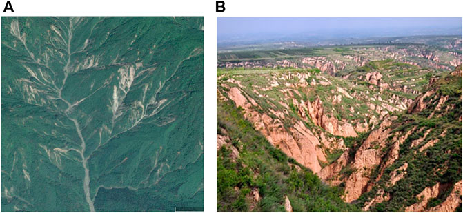
FIGURE 1. (A) Catchment with water erosion at the Baisha River Basin in Dujiangyan, Sichuan, China; (B) gravity erosion region.

Methodology

The Test Setup Parameters

This study examined water erosion and gravity erosion as the common types of soil erosion. Figure 2 shows the geometric models. The water erosion model consists of the slope, gully, and Reaches A and B. The particles on the slope surface enter the gully via runoff and are then transported to the river. The slopes are variable and set at 5°, 15°, and 30°. The degree of the gully is 5°. The slopes of Reaches A and B are 5% and 1%, respectively. The model has four monitoring sections: CS1 at the exit of the slopes, CS2 at the confluence entry of the river, CS3 at the connection of the upper and the lower reaches, and CS4 at the end of the reach. The incoming flow rate on one side of the slope for the water erosion runs is 5 × 10⁻³ m³/s.

FIGURE 2

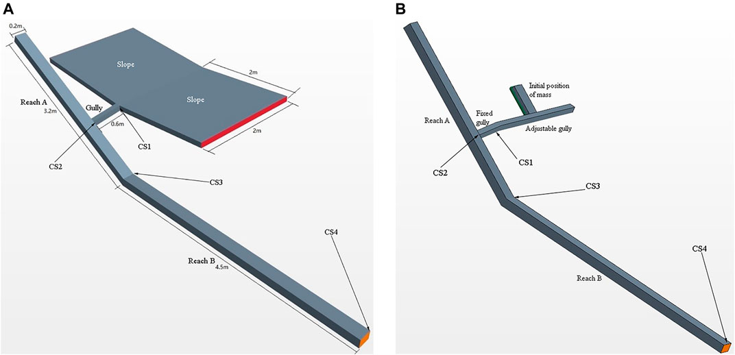
FIGURE 2. Geometric models: (A) water erosion model; (B) gravity erosion model.

In the geometric model of gravity erosion, the slopes in water erosion cases are replaced with an adjustable gully. The fixed gully and Reaches A and B are within the same parameters as in the water erosion model. The particles first enter the adjustable gully with a variable slope of 5°, 15°, and 30° after sliding down from the initial area. Then, the particles enter the fixed gully. The incoming flow rate of the gully is 1 × 10⁻³ m³/s.

Overall, the essential elements of this study are shown in Figure 3.

FIGURE 3

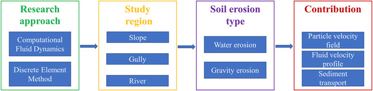
FIGURE 3. Methodological flow chart.

Governing Equations of Fluid Flow

In this simulation, the fluid phase is described by the continuity and momentum equations:

$\frac{\partial \rho }{\partial t}+\nabla \cdot \rho \mathit{u}=0,(1)$

$\frac{\partial }{\partial t}\int \int {\int }_{CV}\rho \mathit{u}\text{dV}+{\displaystyle {∯}_{CS}\rho \mathit{uu}\cdot \mathit{n}\text{dS}}=F_B+F_S,(2)$

where ρ is the fluid density, $\mathit{u}$ is the fluid interstitial velocity, $\mathit{n}$ is the unit normal vector, $F_B$ is the mass force, and$F_S$ is the surface force.

Turbulence simulations are performed using the realizable k–ε turbulence model, where k is the turbulent kinetic energy and ε is the dissipation rate. It is a two-equation turbulence model that allows the turbulence length and time scale to be determined by solving two independent transport equations. The realizable k–ε model provides some improvements to the standard k–ε model (Launder and Spalding, 1972) by removing the values in the calculation results that are contrary to the laws of physics (Shih et al., 1995). Furthermore, it exhibits superior performance for flows involving rotation, boundary layers under strong adverse pressure gradients, separation, and recirculation. Realizable k–ɛ model shows a great ability to capture the mean flow of the complex structures. It is expressed as follows:

$\frac{\partial }{\partial t}\left(\rho k\right)+\frac{\partial }{\partial x_i}\left(\rho k{u}_i\right)=\frac{\partial }{\partial x_j}\left[\left(\mu +\frac{{\mu }_t}{{\sigma }_k}\right)\frac{\partial k}{\partial x_j}\right]+G_k+G_b-\rho \epsilon -Y_M+S_k,(3)$

$\frac{\partial \left(\rho \epsilon \right)}{\partial t}+\frac{\partial }{\partial x_i}\left(\rho \epsilon u_i\right)=\frac{\partial }{\partial x_j}\left[\left(\mu +\frac{{\mu }_t}{{\text{σ}}_{\epsilon }}\right)\frac{\partial \epsilon }{\partial x_j}\right]+\rho C_{1}S\epsilon -\rho C_2\frac{{\epsilon }^2}{k+\sqrt{\frac{{\mu }_t\epsilon }{\rho }}} +C_{1\epsilon }\frac{\epsilon }{k}{C}_{3g}{G}_b+S_{\epsilon },(4)$

where k is the turbulent kinetic energy, μ is the dynamic viscosity, ${\mu }_t$ is the eddy viscosity, and ε is the turbulent dissipation rate.

Mathematical Model of Particle Motion

The particle motion includes translational and rotational movement. According to Newton’s second law of motion, the equations are as follows:

$m\frac{d{v}_a}{dt}=mg+F_{f,a}+{\displaystyle \sum }_{b=1}^n\left(F_{n,ab}+F_{t,ab}\right),(5)$

$I\frac{d\Omega }{dt}={\displaystyle \sum }_{b=1}^n{T}_{ab},(6)$

where m is the mass of a single particle; $v_a$ is the translational velocity; $F_{f,a}$ is the fluid force acting on particle a; and $F_{n,ab}$, $F_{t,ab}$, and $T_{ab}$ are the normal contact force, tangential contact force, and torque between particles a and b, respectively.

Particle contact model is the Hertz–Mindlin soft-sphere model. The normal force ${\mathit{F}}_{n,ij}$ and tangential force ${\mathit{F}}_{t,ij}$ between the particles can be expressed as follows:

${\mathit{F}}_{n,ij}=\left(-k_n{\alpha }^{3/2}-{\eta }_{n,i}\mathit{Gn}\right)\mathit{n},(7)$

${\mathit{F}}_{t,ij}=-k_t\mathit{\delta }-{\eta }_{t,j}{\mathit{G}}_{ct},(8)$

where α is the normal overlap between particles; G is the relative motion velocity of particles i and j; ${\mathit{G}}_{ct}$ is the slip velocity of the contact point; δ is the tangential displacement of the contact point; $k_n$ and $k_t$ are the elasticity coefficients of particle i in the normal and tangential directions, respectively; n is the unit vector from the spherical center of particle i to the spherical center of particle j; and ${\eta }_{n,i}$ and ${\eta }_{t,j}$ are the damping coefficients of the particles in the normal and tangential directions, respectively.

Fluid–Particle Interactions

CFD-DEM coupling involves the following steps. First, the CFD performs fluid field calculation in a time step. Then, the information of the fluid field is delivered to the DEM module to calculate the forces between the two phases. Next, the particle motion is updated by receiving the obtained forces. For a calculation cycle, the fluid field is calculated based on the updated two-phase interaction forces by adding a source term to the fluid momentum equation. Different time steps setting in CFD and DEM will improve the efficiency of the coupling model significantly (Lei et al., 2019). In this study, the ratio was set at 1:100. The simulation parameters are listed in Table 1.

TABLE 1

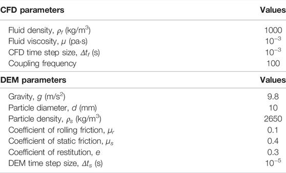
TABLE 1. Parameters of the simulation.

Model Validation

To verify the current numerical implementation, the model was tested against some experimental datasets. Figure 4 shows the comparison between the numerical results and experimental data for the velocity profile and sediment transport. The streamwise velocity profiles were measured using traditional detailed experiment series (Onishi, 1972) and modern instruments (Revil-Baudard et al., 2015) in a laboratory. The sediment transport rate data were obtained through laboratory experiments (Deng et al., 2008) and river gauging stations (Chen et al., 2011). The comparison shows that the numerical results in this research are in good agreement with the experimental data. Thus, the validity of the model was confirmed.

FIGURE 4

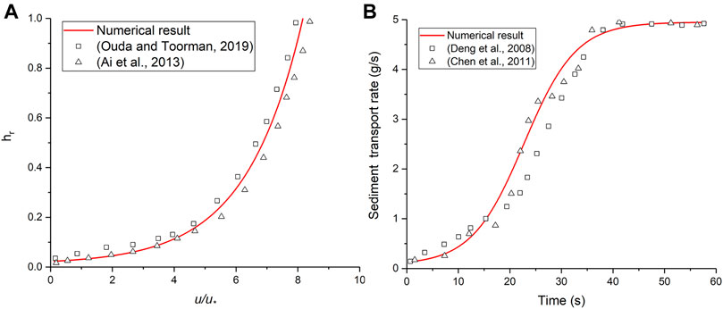
FIGURE 4. Comparison between observed and simulated results: (A) velocity profile; (B) sediment transport rate.

Results

Sediment Transport Following Water Erosion

In order to study the whole process of sediment transport from the slope until it enters the river, the velocity of particle movement needs to be analyzed (Figure 5). The particles start to move at the initial stage because of water flow. As time progresses, the velocity of particles on the slope gradually increases and the particles begin to accumulate in the region between the two slopes. The velocities of particles at different locations were approximately the same, most of them being <0.05 m/s before 1.0s. The velocities of particles at different locations began to appear differently. The velocity of particles near the upper slope was greater by about 0.2 m/s at 1.5s. The velocity of particles further increased, and the velocity of particles in the upper slope was close to 0.5 m/s at 2.0s. The particles arriving in the interslope region start to get carried because of water at 2.5s. The velocity of particles in the gully is greater, mostly exceeding 1 m/s and reaching up to 1.7 m/s. When the particle movement on the slope continues, particle accumulation occurs at the bottom of the slopes, causing the overall velocity on the slope to slow down. The particles enter the river from 3.5s, and the particle velocity in the gully increases further to a maximum value of 4.0 m/s. The velocity of particles in the upstream reach is about 2.7∼4.0 m/s and greater than that in the downstream reach due to a greater slope gradient. The velocity in the downstream reach is about 1.4∼2.8 m/s. The particles’ velocity on the slope decreases from 5.0s and eventually drops to a very small value.

FIGURE 5

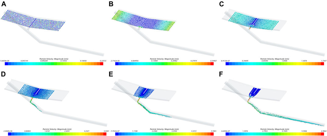
FIGURE 5. Particle velocity field, water erosion: (A) t = 0.5s; (B) t = 1.5s; (C) t = 2.5s; (D) t = 3.5s; (E) t = 5s; (F) t = 7s.

Figure 6 shows the streamwise velocity profile when the slope is 5°. The friction velocity is $u_{\ast }=\sqrt{\tau /\rho }$, where τ is the shear stress and ρ is the fluid density. The maximum flow velocity in the CS1 is close to 4 $u_{\ast }$. The fluid velocity at the bottom is very small because of the particle motion. When the relative water depth h_r reaches 0.7, the streamwise velocity increases rapidly. The velocity distribution throughout the sediment transport process does not change much in this section. The velocity at the bottom of the CS2 is small, and there is a small increase in the interval of 0∼0.6 h_r. The velocity curve is steep at 1.0s. The slope of the velocity curve gradually decreases from 2.0 to 8.0s. CS3 and CS4 are in the river. The streamwise velocity conforms to the law of logarithmic distribution from 1.0s to 3.0s. As the sediment transport rate increases, the solid phase has an important influence on the flow velocity distribution. The velocity decreases to some extent in the bottom region and gradually increases from bottom to top at 4.0s. At 7.0 and 8.0s, the velocity at the bottom decreases significantly.

FIGURE 6

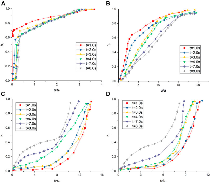
FIGURE 6. Streamwise velocity profile of fluid, water erosion: (A) CS1; (B) CS2; (C) CS3; (D) CS4.

The sediment transport of water erosion cases is shown in Figure 7. When the slope gradient is 5°, the particles pass through the exit of slope (CS1) at 2.28s. Thereafter, the sediment transport rate increases rapidly from 2.28 to 4.46s, reaching a peak of 1.9 × 10⁻⁴ kg/(s m) at 4.46s. The time particles take to enter the gully through the CS2 is 2.7s, after which the sediment transport rate increases rapidly from 2.7 to 4.02s and reaches the maximum value of 2.4 × 10⁻⁴ kg/(s m) at 4.02s. This is 27% higher than the peak of sediment transport rate in CS1. The time when particles enter the downstream reach (CS3) is 3.66, and the peak of the sediment transport rate is 1.8 × 10⁻⁴ kg/(s m). The moment when particles reach the ending section (CS4) is 7.02s, and the sediment transport rate reaches the peak of 2.8 × 10⁻⁴ kg/(s m), which is 49% higher than the peak at CS1.

FIGURE 7

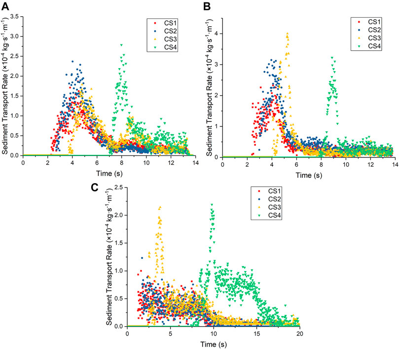
FIGURE 7. Sediment transport, water erosion: (A) slope degree: 5°; (B) slope degree: 15°; (C) slope degree: 30°.

When the slope is 15°, the sediment transport rate at all sections increases rapidly at the beginning, decreases after reaching the peak, and finally stabilizes at a lower range. The peak of sediment transport rate at CS1 is the smallest. The peaks at CS2 and CS4 are very close, which are 35% and 39% higher than CS1, respectively. The peak at CS3 is the greatest, which is 72% higher than CS1.

When the slope is 30°, the variation of sediment transport rate is different from that of the 5° and 15° slopes. The sediment transport rates at CS1 and CS2 show no obvious increasing and decreasing processes. They fluctuate continuously in the range of 0–1 × 10⁻⁴ kg/(s m). A dramatic increase and decrease still exist at CS3 and CS4. The sediment transport rate of CS3 has a double-peak process. The first peak occurs at the beginning of sediment transport, which is 1.3 × 10⁻⁴ kg/(s m). Thereafter, it decreases to near 0, rises rapidly again, and reaches the second peak of 2.1 × 10⁻⁴ kg/(s m). The sediment transport rate peak at CS4 is 2.2 × 10⁻⁴ kg/(s m). In the decreasing process, the sediment transport rate fluctuates in the interval of 10.5s to 14s.

Sediment Transport Following Gravity Erosion

The particle velocity field for gravity erosion is shown in Figure 8. When the particles slide down and enter the gully, the maximum velocity is 0.46 m/s. When the particles cover the gully entrance area, the maximum velocity of the particles reaches 0.54 m/s. Many particles are transported in the gully, and their velocity is greater than that of the particles still in the initial area at 1.5s. At 2.0s, all particles enter the gully and few particles begin to enter the river. The maximum velocity of particles is 2 m/s. Most particles enter the river, and a small number of particles go to Reach B at 3.0s. The maximum velocity of particles is 2.1 m/s. Once most of the particles have entered Reach B, the maximum velocity is reduced to 1.5 m/s at 4.0s. The particles are transported in Reach B, and the maximum velocity is 1.3 m/s at 6.0s. Some particles are transported out of the study reach, and the maximum velocity is 1.2 m/s at 8.0s.

FIGURE 8

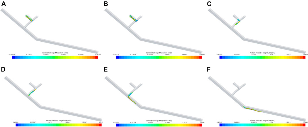
FIGURE 8. Particle velocity field, gravity erosion: (A) t = 0.5s; (B) t = 1s; (C) t = 1.5s; (D) t = 2s; (E) t = 2.5s; (F) t = 4s.

Figure 9 shows the fluid streamwise velocity profiles for gravity erosion when the adjustable gully is 5°. The particles enter the gully from the initial region at 1.0s. Because CS1 is close to the initial region, the velocity distribution is affected immediately. It no longer conforms to the logarithmic distribution. An approximately linear increase from the bottom up appears in the range of h_r < 0.5. When h_r exceeds 0.5, the increase is small. The overall velocity decreases due to the influence of sediment transport at 2.0s. The sediment transport process ends and the velocity profile almost returns to a logarithmic response at 4.0s. The section is no longer affected by solid particle sediment transport, and the velocity profile is logarithmic at 7.0 and 8.0s. The flow velocity of CS2 gradually decreases from 1.0 to 3.0s as the sediment transport proceeds. The particles have all passed through the section at 4.0s, and the liquid phase velocity increases. The flow velocity is no longer affected by the particles, and the velocity profile is in line with the logarithmic distribution at 7.0 and 8.0s. In CS3, sediment transport did not occur and velocity profile was logarithmic at 1.0s and 2.0s. A large number of particles pass through the section, causing a significant change in velocity profile at 3.0s and 4.0s. The velocity near the bottom decreases significantly and increases rapidly near h_r = 0.3. After h_r > 0.4, it increases linearly up to the surface. The sediment transport process ends, and the velocity distribution returns to logarithmic distribution at 7.0s and 8.0s. In CS4, the flow velocity decreases from 1.0s to 4.0s, but all profiles conform to the logarithmic distribution. Influenced by the solid phase at 7.0s and 8.0s, the velocity curve can be divided into three parts. When h_r < 0.3, the flow velocity slowly increases upward from the bottom; when 0.3 < h_r < 0.6, the flow velocity increases rapidly from the bottom to the top; when h_r > 0.6, the flow velocity increases slowly.

FIGURE 9

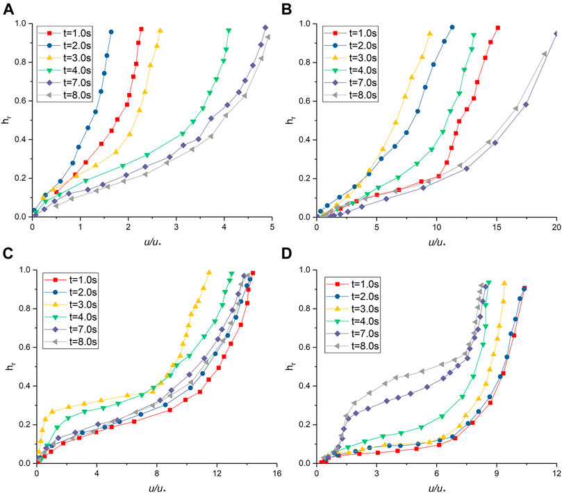
FIGURE 9. Fluid velocity profile, gravity erosion: (A) CS1; (B) CS2; (C) CS3; (D) CS4.

For the subsequent sediment transport process of gravity erosion, the changing processes of sediment transport rate are similar when adjustable gully is 5°, 15°, and 30° (Figure 10). All of them are single-peaked. The duration of the sediment transport process and the maximum sediment transport rate at CS1–CS4 are presented in Table 2. The sediment transport process is short in this case because of the rapid sediment yield process. The durations of sediment transport decrease in order from CS4 to CS1. The peaks of the sediment transport rate at CS1 and CS2 are near the end of the sediment transport process (the teak time positions are >0.8), whereas those of CS3 and CS4 are in the middle and late stages (peak time position: 0.53–0.66). The peak value of the sediment transport rate gradually decreases from CS1 to CS4. The peaks in CS2, CS3, and CS4 are 78%–92%, 45%–50%, and 19%–24% of the peak in CS1, respectively. The increase in adjustable gully slope will accelerate the sediment transport and significantly increase the sediment transport rate peak.

FIGURE 10

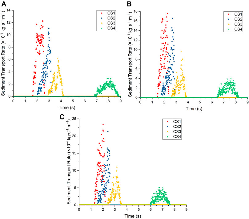
FIGURE 10. Sediment transport, gravity erosion: (A) adjustable gully slope: 5°; (B) adjustable gully slope: 15°; (C) adjustable gully slope: 30°.

TABLE 2

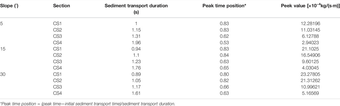
TABLE 2. The time of sediment transport and peek.

Discussion

Water erosion and gravity erosion are two main forms of soil erosion, exhibiting different subsequent sediment transport processes. The particle and fluid velocities and sediment transport were studied using many new physical equipment, such as an Acoustic Doppler Current Profiler and Particle Image Velocimetry (Kostaschuk et al., 2005; Corapi et al., 2021). Our results show the same laws and trends with these study in general, however, the specific quantities and processes are different. The sediment transport duration following gravity erosion is short. The velocity of particles in gravity erosion is greater than that in water erosion at the early stage.

The velocity profile in this study differs in terms of the multiphase sediment transport mode based on the modified volume of fluid equation (Ouda and Toorman, 2019). It is not influenced by the solid phase and conforms to the logarithmic distribution. The main reason is that the turbulence closure term is handled differently. The logarithmic velocity distribution holds overall and is consistent with the other numerical simulations (Ai et al., 2013; Charru et al., 2016). Sediment transport influences the fluid velocity and its distribution. CS1 and CS2 are at the inlet and outlet of the gully. In gravity erosion cases, the flow velocity of the whole section is reduced, and the velocity profile returns to logarithmic distribution at the end. In the cases of water erosion, velocity decreases in the lower layer, especially near the bottom, and the flow velocity distribution does not return to logarithmic distribution because of the continuous sediment transport process. CS3 and CS4 are in the river. The velocity near the bottom is small; increases significantly from the bottom to top in the middle; and increases slowly in the upper layers.

According to the experimental study, slope gradient has significant effects on sediment transport (Lin et al., 2017). Previous studies focused on the spatial distribution of transport rates (Istanbulluoglu et al., 2003; Dai et al., 2021) and the assessment of the sediment sources (Lin et al., 2015). In this study, the temporal features of sediment transport were investigated. Gravity and water erosion cases involve different sediment transport processes. The gravity erosion process often has a steep rise and fall in the sediment transport rate. The peak of sediment transport rate decreases from CS1 to CS4. The sediment transport process in CS4 takes a long time, but the peak is low because the concentration, particle stress, and Reynolds stress are all significant influential factors (Schmeeckle, 2014). In gravity erosion cases, the gradient of adjustable gully does not affect the shape of the sediment transport process. However, in the cases of water erosion, the gradient of the slope has a significant effect on the sediment transport process.

The comparison of the numerical simulation approaches is listed in Table 3. The advantage of CFD-DEM is that it can realistically simulate the phases in a multiphase flow. In practical applications, attention should be paid to the huge quantity of computation due to the large number of particles in granular phase solution as well as the difficulties of accurately calculating the fluid volume fraction and determining the drag force between the liquid and solid phases.

TABLE 3

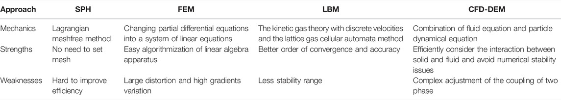
TABLE 3. Comparison of numerical simulation approaches.

Conclusion

This study presents numerical investigations of sediment transport in the gully and reach using CFD-DEM coupled simulations. The sediment transport following different types of soil erosion was examined. The particle velocity fields, fluid velocity distribution, and sediment transport processes were analyzed. The main conclusions are as follows.

Comparing the particle velocities in water erosion and gravity erosion cases, the particle velocity in gravity erosion is greater than that in water erosion at the beginning of the sediment transport process. The reason is that more potential energy is converted into kinetic energy when gravity erosion occurs. Water erosion has more sediment yield, and the sediment transport process lasts longer.

The streamwise fluid velocity profile conforms to the logarithmic distribution when it is not affected by solid-phase particles. When the sediment transport process starts, the fluid velocity distribution changes. In the cases of water erosion, the bottom flow velocity is very small in the first two sections, while the flow velocity in the river sections gradually increases from the bottom to the top. In the cases of gravity erosion, the streamwise velocity at the first two sections decreases in vertical direction and the flow velocity at the bottom of the sections in the river decreases significantly.

The occurrence of the sediment transport rate following water erosion is closely related to the gradient of the slope. The peak exists for the 5° and 15° slope cases but not for the 30° slope case. When the slope is 5°, the second peak occurs at the connection between two reaches. When the slope is 30°, the declining process shows a step form in river sections. The sediment transport rate peaks following gravity erosion are large at the gully inlet and outlet, whereas they are relatively low in the river sections. The sediment transport rate peak increases and the sediment transport duration reduces with the increase of gully gradient. The sediment transport curve shape is not affected by the gully gradient.

Data Availability Statement

The original contributions presented in the study are included in the article/supplementary material. Further inquiries can be directed to the corresponding author.

Author Contributions

YL: numerical simulation, analysis, and writing. ZY: software and validation. XW: supervision, conceptualization, and funding acquisition.

Funding

The study is supported by the National Natural Science Foundation of China (Grant No. 51639007).

Conflict of Interest

The authors declare that the research was conducted in the absence of any commercial or financial relationships that could be construed as a potential conflict of interest.

The reviewer CL declared a shared affiliation with the authors to the handling editor at the time of review.

Publisher’s Note

All claims expressed in this article are solely those of the authors and do not necessarily represent those of their affiliated organizations, or those of the publisher, the editors and the reviewers. Any product that may be evaluated in this article, or claim that may be made by its manufacturer, is not guaranteed or endorsed by the publisher.

References

Ai, C., Jin, S., and Xing, Y. (2013). Influence of Suspended Load on 3D Numerical Simulation of Flow and Bed Evolution in a Meandering Channel Bend. J. Hydraul. Eng. 139, 450–455. doi:10.1061/(asce)hy.1943-7900.0000691

CrossRef Full Text | Google Scholar

Asadi, E., Isazadeh, M., Samadianfard, S., Ramli, M. F., Mosavi, A., Nabipour, N., et al. (2020). Groundwater Quality Assessment for Sustainable Drinking and Irrigation. Sustainability 12 (1), 177. doi:10.3390/su12010177

CrossRef Full Text | Google Scholar

Band, S. S., Janizadeh, S., Chandra Pal, S., Saha, A., Chakrabortty, R., Shokri, M., et al. (2020b). Novel Ensemble Approach of Deep Learning Neural Network (DLNN) Model and Particle Swarm Optimization (PSO) Algorithm for Prediction of Gully Erosion Susceptibility. Sensors (Basel) 20, 5609. doi:10.3390/s20195609

PubMed Abstract | CrossRef Full Text | Google Scholar

Band, S. S., Janizadeh, S., Pal, S. C., Saha, A., Chakrabortty, R., Melesse, A. M., et al. (2020a). Flash Flood Susceptibility Modeling Using New Approaches of Hybrid and Ensemble Tree-Based Machine Learning Algorithms. Remote Sens. 12, 3568. doi:10.3390/rs12213568

CrossRef Full Text | Google Scholar

Bennett, J. P. (1974). Concepts of Mathematical Modeling of Sediment Yield. Water Resour. Res. 10, 485–492. doi:10.1029/wr010i003p00485

CrossRef Full Text | Google Scholar

Cai, J. Y., Zhou, Z. H., Liu, J. J., Wang, H., Jia, Y. W., and Xu, C. Y. (2019). A Three-Process-Based Distributed Soil Erosion Model at Catchment Scale on the Loess Plateau of China. J. Hydrology 578, 124005. doi:10.1016/j.jhydrol.2019.124005

CrossRef Full Text | Google Scholar

Charru, F., Bouteloup, J., Bonometti, T., and Lacaze, L. (2016). Sediment Transport and Bedforms: A Numerical Study of Two-Phase Viscous Shear Flow. Meccanica 51, 3055–3065. doi:10.1007/s11012-016-0553-5

CrossRef Full Text | Google Scholar

Chen, C.-N., Tsai, C.-H., and Tsai, C.-T. (2011). Simulation of Runoff and Suspended Sediment Transport Rate in a Basin with Multiple Watersheds. Water Resour. Manage 25, 793–816. doi:10.1007/s11269-010-9727-4

CrossRef Full Text | Google Scholar

Choubin, B., Mosavi, A., Alamdarloo, E. H., Hosseini, F. S., Shamshirband, S., Dashtekian, K., et al. (2019). Earth Fissure Hazard Prediction Using Machine Learning Models. Environ. Res. 179, 108770. doi:10.1016/j.envres.2019.108770

PubMed Abstract | CrossRef Full Text | Google Scholar

Corapi, P., Chacon, X. C. A., Acaro Chacón, X. C., and Chuquimarca Jimenez, L. E. (2021). Velocity Scaling in Open-Channel Flows with Sediment Transport. Tecnol. Cienc. Agua 12, 53–110. doi:10.24850/j-tyca-2021-05-02

CrossRef Full Text | Google Scholar

Cui, S. H., Pei, X. J., Jiang, Y., Wang, G. H., Fan, X. M., Yang, Q. W., et al. (2021). Liquefaction within a Bedding Fault: Understanding the Initiation and Movement of the Daguangbao Landslide Triggered by the 2008 Wenchuan Earthquake (Ms=8.0). Eng. Geol. 295, 106455. doi:10.1016/j.enggeo.2021.106455

CrossRef Full Text | Google Scholar

Dai, W., Xiong, L. Y., Antoniazza, G., Tang, G. A., and Lane, S. N. (2021). Quantifying the Spatial Distribution of Sediment Transport in an Experimental Gully System Using the Morphological Method. Earth Surf. Process. Landforms 46, 1188–1208. doi:10.1002/esp.5094

CrossRef Full Text | Google Scholar

Dang, S. Z., Liu, X. Y., Yin, H. J., and Guo, X. W. (2020). Prediction of Sediment Yield in the Middle Reaches of the Yellow River Basin under Extreme Precipitation. Front. Earth Sci. 8, 542686. doi:10.3389/feart.2020.542686

CrossRef Full Text | Google Scholar

Deng, Z.-Q., De Lima, J. L. M. P., and Jung, H.-S. (2008). Sediment Transport Rate-Based Model for Rainfall-Induced Soil Erosion. Catena 76, 54–62. doi:10.1016/j.catena.2008.09.005

CrossRef Full Text | Google Scholar

Elghannay, H., and Tafti, D. (2018). LES-DEM Simulations of Sediment Transport. Int. J. Sediment Res. 33, 137–148. doi:10.1016/j.ijsrc.2017.09.006

CrossRef Full Text | Google Scholar

Gao, H., Xu, X., Zhang, H., Jiang, Y., and Zhao, T. (2020). How Effective Is Vegetation in Reducing Gravity Erosion on Loess Gully Sidewall under Intense Rainfalls? Land Degrad. Dev. 31, 2605–2619. doi:10.1002/ldr.3634

CrossRef Full Text | Google Scholar

Guo, W., Xu, X., Zhu, T., Zhang, H., Wang, W., Liu, Y., et al. (2020b). Changes in Particle Size Distribution of Suspended Sediment Affected by Gravity Erosion: A Field Study on Steep Loess Slopes. J. Soils Sediments 20, 1730–1741. doi:10.1007/s11368-019-02496-z

CrossRef Full Text | Google Scholar

Guo, W., Xu, X. Z., Wang, W. L., Zhu, T. X., and Liu, Y. K. (2020a). Experimental Study of Shallow Mass Movements on Gully Slopes and Associated Sediment under Rainfall on the Chinese Loess Plateau. Geomorphology 350, 106919. doi:10.1016/j.geomorph.2019.106919

CrossRef Full Text | Google Scholar

Istanbulluoglu, E., Tarboton, D. G., Pack, R. T., and Luce, C. (2003). A Sediment Transport Model for Incision of Gullies on Steep Topography. Water Resour. Res. 39, 1103. doi:10.1029/2002wr001467

CrossRef Full Text | Google Scholar

Kandel, D. D., Western, A. W., Grayson, R. B., and Turral, H. N. (2004). Process Parameterization and Temporal Scaling in Surface Runoff and Erosion Modelling. Hydrol. Process. 18, 1423–1446. doi:10.1002/hyp.1421

CrossRef Full Text | Google Scholar

Kostaschuk, R., Best, J., Villard, P., Peakall, J., and Franklin, M. (2005). Measuring Flow Velocity and Sediment Transport with an Acoustic Doppler Current Profiler. Geomorphology 68, 25–37. doi:10.1016/j.geomorph.2004.07.012

CrossRef Full Text | Google Scholar

Launder, B. E., and Spalding, D. B. (1972). Mathematical Models of Turbulence. Sint-Genesius-Rode, Belgium: Von Karman Institute for Fluid Dynamics.

Google Scholar

Lei, M., Xu, Z.-X., Zhao, T., and Wang, X.-K. (2019). Dynamics of Loose Granular Flow and its Subsequent Deposition in a Narrow Mountainous River. J. Mt. Sci. 16, 1367–1380. doi:10.1007/s11629-018-5080-5

CrossRef Full Text | Google Scholar

Lei, M., Yang, P., Wang, Y. K., and Wang, X. K. (2020). Numerical Analyses of the Influence of Baffles on the Dynamics of Debris Flow in a Gully. Arabian J. Geosci. 13, 1052. doi:10.1007/s12517-020-06016-z

CrossRef Full Text | Google Scholar

Li, H., Deng, J., Yuan, S., Feng, P., and Arachchige, D. D. K. (2021a). Monitoring and Identifying Wind Turbine Generator Bearing Faults Using Deep Belief Network and EWMA Control Charts. Front. Energy Res. 9, 799039. doi:10.3389/fenrg.2021.799039

CrossRef Full Text | Google Scholar

Li, H. J., Deng, J. H., Feng, P., Pu, C. H., Arachchige, D. D. K., and Cheng, Q. (2021b). Short-Term Nacelle Orientation Forecasting Using Bilinear Transformation and ICEEMDAN Framework. Front. Energy Res. 9, 780928. doi:10.3389/fenrg.2021.780928

CrossRef Full Text | Google Scholar

Li, H. (2022a). SCADA Data Based Wind Power Interval Prediction Using LUBE-Based Deep Residual Networks. Front. Energy Res. 10, 920837. doi:10.3389/fenrg.2022.920837

CrossRef Full Text | Google Scholar

Li, H. (2022b). Short-Term Wind Power Prediction via Spatial Temporal Analysis and Deep Residual Networks. Front. Energy Res. 10, 920407. doi:10.3389/fenrg.2022.920407

CrossRef Full Text | Google Scholar

Li, T., Wang, G., Xue, H., and Wang, K. (2009). Soil Erosion and Sediment Transport in the Gullied Loess Plateau: Scale Effects and Their Mechanisms. Sci. China Ser. E-Technol. Sci. 52, 1283–1292. doi:10.1007/s11431-009-0076-6

CrossRef Full Text | Google Scholar

Lin, J., Huang, Y., Wang, M.-k., Jiang, F., Zhang, X., and Ge, H. (2015). Assessing the Sources of Sediment Transported in Gully Systems Using a Fingerprinting Approach: An Example from South-East China. Catena 129, 9–17. doi:10.1016/j.catena.2015.02.012

CrossRef Full Text | Google Scholar

Lin, J., Huang, Y., Zhao, G., Jiang, F., Wang, M.-k., and Ge, H. (2017). Flow-Driven Soil Erosion Processes and the Size Selectivity of Eroded Sediment on Steep Slopes Using Colluvial Deposits in a Permanent Gully. Catena 157, 47–57. doi:10.1016/j.catena.2017.05.015

CrossRef Full Text | Google Scholar

Onishi, Y. (1972). Effects of Meandering on Sediment Discharges and Friction Factors of Alluvial Streams. Iowa: The University of Iowa.

Google Scholar

Ouda, M., and Toorman, E. A. (2019). Development of a New Multiphase Sediment Transport Model for Free Surface Flows. Int. J. Multiph. Flow 117, 81–102. doi:10.1016/j.ijmultiphaseflow.2019.04.023

CrossRef Full Text | Google Scholar

Poesen, J. (2018). Soil Erosion in the Anthropocene: Research Needs. Earth Surf. Process. Landforms 43, 64–84. doi:10.1002/esp.4250

CrossRef Full Text | Google Scholar

Qasem, S. N., Samadianfard, S., Nahand, H. S., Mosavi, A., Shamshirband, S., and Chau, K. W. (2019). Estimating Daily Dew Point Temperature Using Machine Learning Algorithms. Water 11, 582. doi:10.3390/w11030582

CrossRef Full Text | Google Scholar

Revil-Baudard, T., Chauchat, J., Hurther, D., and Barraud, P.-A. (2015). Investigation of Sheet-Flow Processes Based on Novel Acoustic High-Resolution Velocity and Concentration Measurements. J. Fluid Mech. 767, 1–30. doi:10.1017/jfm.2015.23

CrossRef Full Text | Google Scholar

Romshoo, S. A., Yousuf, A., Altaf, S., and Amin, M. (2021). Evaluation of Various DEMs for Quantifying Soil Erosion under Changing Land Use and Land Cover in the Himalaya. Front. Earth Sci. 9, 782128. doi:10.3389/feart.2021.782128

CrossRef Full Text | Google Scholar

Schmeeckle, M. W. (2014). Numerical Simulation of Turbulence and Sediment Transport of Medium Sand. J. Geophys. Res. Earth Surf. 119, 1240–1262. doi:10.1002/2013jf002911

CrossRef Full Text | Google Scholar

Shabani, S., Samadianfard, S., Sattari, M. T., Mosavi, A., Shamshirband, S., Kmet, T., et al. (2020). Modeling Pan Evaporation Using Gaussian Process Regression K-Nearest Neighbors Random Forest and Support Vector Machines; Comparative Analysis. Atmosphere 11, 1–17. doi:10.3390/atmos11010066

CrossRef Full Text | Google Scholar

Shih, T. H., Liou, W. W., Shabbir, A., Yang, Z., and Zhu, J. (1995). A New k-ϵ Eddy Viscosity Model for High Reynolds Number Turbulent Flows. Comput. Fluids 24, 227–238.

CrossRef Full Text | Google Scholar

Sirjani, E., Mahmoodabadi, M., and Cerdà, A. (2022). Sediment Transport Mechanisms and Selective Removal of Soil Particles under Unsteady-State Conditions in a Sheet Erosion System. Int. J. Sediment Res. 37, 151–161. doi:10.1016/j.ijsrc.2021.09.006

CrossRef Full Text | Google Scholar

Sterk, G. (2021). A Hillslope Version of the Revised Morgan, Morgan and Finney Water Erosion Model. Int. Soil Water Conserv. Res. 9, 319–332. doi:10.1016/j.iswcr.2021.01.004

CrossRef Full Text | Google Scholar

Sun, R., and Xiao, H. (2016). SediFoam: A General-Purpose, Open-Source CFD-DEM Solver for Particle-Laden Flow with Emphasis on Sediment Transport. Comput. Geosci. 89, 207–219. doi:10.1016/j.cageo.2016.01.011

CrossRef Full Text | Google Scholar

Sun, R., Xiao, H., and Sun, H. (2017). Realistic Representation of Grain Shapes in CFD-DEM Simulations of Sediment Transport with a Bonded-Sphere Approach. Adv. Water Resour. 107, 421–438. doi:10.1016/j.advwatres.2017.04.015

CrossRef Full Text | Google Scholar

Wu, S. B., Chen, L., Wang, N. L., Zhang, J., Wang, S. Q., Bagarello, V., et al. (2021). Variable Scale Effects on Hillslope Soil Erosion during Rainfall-Runoff Processes. Catena 207, 105606. doi:10.1016/j.catena.2021.105606

CrossRef Full Text | Google Scholar

Xu, X.-Z., Zhang, H.-W., Wang, W.-L., Zhao, C., and Yan, Q. (2015). Quantitative Monitoring of Gravity Erosion Using a Novel 3D Surface Measuring Technique: Validation and Case Study. Nat. Hazards 75, 1927–1939. doi:10.1007/s11069-014-1405-z

CrossRef Full Text | Google Scholar

Zhang, L. C., Liu, X. J., Song, Y. J., Li, J., Cai, C. F., Zhao, X. M., et al. (2021). Characterization of Surface Runoff Pathways and Erosion Using Hydrological Attributes under Simulated Rainfall. Front. Earth Sci. 9, 683473. doi:10.3389/feart.2021.683473

CrossRef Full Text | Google Scholar