 Jakob Gallistl
 Daniel Schwindt
 Jochum Birgit4
95% of researchers rate our articles as excellent or good
Learn more about the work of our research integrity team to safeguard the quality of each article we publish.
Find out more
ORIGINAL RESEARCH article
Front. Earth Sci. , 12 September 2022
Sec. Hydrosphere
Volume 10 - 2022 | https://doi.org/10.3389/feart.2022.911611
This article is part of the Research Topic Advances in the Application of Multi-Dimensional Geophysical Surveys in Earth and Environmental Sciences View all 8 articles
We present an approach that permits to predict hydraulic conductivity from extensive, multi-methodical geophysical data collected on a hillslope affected by landslides in Austria. The objective of the investigation is the spatial characterization of a slope affected by mass movements to derive hydrogeological structures and preferential flow paths. The geophysical data sets presented in this study consists of 24 densely distributed complex conductivity (CC) imaging profiles, collocated to these profiles we also collected 517 transient electromagnetic (TEM) soundings and 10 refraction seismic tomography (RST) profiles. Additionally, we also present well-logging data (namely electrical resistivity, natural gamma logs) collected in five boreholes. Cores recovered during the drilling of the boreholes are used to aid in the interpretation of the geophysical units, while analysis of the sediments was conducted to obtain grain size distributions, cation exchange capacity and mineralogy of the subsurface materials. While all geophysical data was processed initially independently, the final complex conductivity imaging results are based on the incorporation of structural constraints about the electrical units obtained from the TEM soundings. The interpretation of the resolved CC units is then sustained by the RST images and the lithological information from the boreholes. We estimate then the hydraulic conductivity of the subsurface derived from the CC images using a two-step approach. In a first step, we investigated the link between the complex conductivity and the different soil volume fractions of gravel, sand, silt and clay. In a second step, we applied a pedo-transfer function, namely the well-known Rosetta model, that permits to predict the hydraulic conductivity from the estimated grain size volumes. This approach allowed a quantitative interpretation of the geophysical data and thus a 3-dimensional (3D) representation of the grain size distribution and hydraulic conductivity in the investigated slope section. Thereby, we observed well-determined site-specific relationships (R2 > 0.7) from the comparison of the complex resistivity images and grain size analysis. The obtained hydrogeophysical 3D model permits to delineate the geometry of an aquiclude, and, thus, the analysis of preferential water-flow paths. In particular, we can identify a spatial correlation between the aquiclude interface and morphological features.
Current forecasts assume that the trend towards rising temperatures and precipitation extremes (Dunn et al., 2020) will continue and that the occurrence of droughts (e.g., Cook et al., 2018; Balting et al., 2021) and heavy rainfall (Ban et al., 2015; Papalexiou and Montanari 2019) can will increase in the next years. Such meteorological changes affect ecosystems (e.g., Weiskopf et al., 2020)), land use (Searchinger et al., 2018), water availability (Konapala et al., 2020), but also natural disasters such as floods (Tabari 2020) and mass movements (Alvioli et al., 2018; Lin et al., 2020). In this context, a comprehensive understanding of the hillslope hydrology is of fundamental importance, to predict runoff responses (Blume and Van Meerveld 2015), but also in the understanding of the hydraulic properties of the subsurface triggering landslide processes (Bogaard and Greco 2016). The complex sedimentary structures in hillslopes, as a result of geological disposition and local geomorphodynamics, make prediction of hydrological processes immensely difficult (Sidle et al., 2019). Small-scale variations in sediment characteristics and the associated hydraulic properties affect infiltration, percolation, but also evaporation (Lehmann et al., 2018) as well as water storage (Berg et al., 2017) and affects hydrologic connectivity via surface runoff and subsurface flow. As a consequence, slope architecture may be related to areas of waterlogging, small-scale slumping or subsidence as well as major mass movements. Moreover, Blume and Van Meerveld (2015) conclude, that the subsurface hillslope-stream connectivity is difficult to observe and quantify, and, due to the high variability in hillslope responses, results are hard to extrapolate to other hillslopes. Blume and Van Meerveld (2015) also point out, that multimethod approaches might be useful, as they strengthen the interpretation of individual measurements.
While the description of hillslope properties is often based on point data from core soundings, a spatial approach is needed to deal with the complexity of the slope sediments and the associated hydrology. In recent years, geophysical methods have been increasingly used to spatially characterize the shallow subsurface (Flores Orozco et al., 2018b; Gallistl et al., 2018; Watlet et al., 2018; Huntley et al., 2019; Holmes et al., 2020). Furthermore, approaches to use geophysical imaging as landslide early warning systems, by monitoring short- and long-term moisture dynamics are developed (Whiteley et al., 2021).
Geophysical methods commonly applied in hillslope characterization include the Electrical Resistivity Tomography (ERT) (Perrone et al., 2014), Refraction Seismic Tomography (RST) (Samyn et al., 2012; Uhlemann et al., 2016), and, to a lesser extent Electromagnetic Induction at low induction number (EMI) (Grandjean et al., 2011; Kušnirák et al., 2016), Transient Electromagnetic Sounding (TEM) (Godio and Bottino, 2001; Li et al., 2020) and Induced Polarization Imaging (IP) (Flores Orozco et al., 2018a; Gallistl et al., 2018; Revil et al., 2020).
IP, also referred to as Complex Conductivity Imaging (CCI), is an extension of the ERT method and provides information about the electrical conductivity and capacitive (polarization) properties of the subsurface (Kemna et al., 2012). The IP method was developed for the prospection of metallic mineral ores given the strong IP response in the presence of iron sulphides (Pelton et al., 1978). In recent years, IP has emerged as a promising method for various environmental and hydrogeological applications including the mapping of geochemical active zones (Flores-Orozco et al., 2020; Katona et al., 2021), the monitoring of changes in pore-space geometry accompanying bioremediation processes (Flores Orozco et al., 2011; Flores Orozco et al., 2019) and the assessment of permafrost degradation (Doetsch et al., 2015; Maierhofer et al., 2022), just to name a few. In the context of characterizing hillslopes affected by landslides, IP has revealed promising results (Flores Orozco et al., 2018a; Gallistl et al., 2018; Revil et al., 2020), as numerous laboratory studies reported a sensitivity of the IP method to soil-textural properties of the subsurface (Slater and Glaser, 2003; Tarasov and Titov, 2007; Revil and Florsch, 2010) and, thus, the improved estimation of hydraulic conductivity (Slater et al., 2014; Weller et al., 2015; Weller and Slater, 2019). Since landslides are frequently triggered by heavy precipitation events, resolving changes in textural properties of hillslopes is of great interest as they will determine areas of low hydraulic conductivity (i.e., with a poor drainage) where pore-pressure may accumulate resulting in the triggering of mass movements (Campbell, 1975; Rogers and Selby, 1980). Thus, IP could permit to directly provide estimates of hydraulic conductivity without the need of direct in-situ testing not possible in landslides. Unfortunately, the upscaling and transferring of laboratory findings to field-scale measurements has proven difficult so far (Binley et al., 2015).
Over the last few decades, a multitude of pedotransfer functions (PTFs) have been developed that permit the prediction of soil-hydraulic properties based on commonly available soil information such as soil texture, bulk density and grain size without the need of labor intensive and time-consuming direct measurements (Van Looy et al., 2017; Zhang and Schaap, 2019). Such PTFs provide a viable alternative, if it is possible to define site-specific equations relating the IP effect to soil texture (i.e., the soil volume fractions of sand, silt, clay and gravel) for a quantitative interpretation of IP imaging results in a hydrogeological context. The predictors in PTFs range from relatively simple power model relations (Cosby et al., 1984) to more complex artificial neural networks (Schaap et al., 2001), support vector machines algorithms (Twarakavi et al., 2009), k-nearest neighbor methods (Nemes et al., 2006) and decision/regression trees (Jorda et al., 2015). Rosetta (Schaap et al., 2001), is one of many PTFs that is based on an artificial neural network and uses a hierarchical approach to predict saturated hydraulic conductivity Ks and van Genuchten (VG) water retention parameters (Van Genuchten, 1980). The model input parameters may be given in terms of textural classes, the soil volume fractions of sand, silt and clay (SSC), or as a combination of SSC, bulk density and a referential grain size. As discussed in Zhang and Schaap (2017) the initial version of Rosetta had several deficiencies, which lead to a weighted re-calibration of Rosetta in order to improve the predicted soil-hydraulic properties and reduce uncertainties in their prediction.
The objective of this work is to investigate the spatial prediction of soil-hydraulic properties at the slope scale, based on derivation of soil texture from complex conductivity information and subsequent use of a pedotransfer function (Rosetta). To the best of our knowledge such approach has not been tested for the interpretation of IP imaging data at the field scale. To reduce the uncertainty in IP inversion results, we also present the incorporation of a priori information about electrical units obtained from TEM data; additionally, we include refraction seismic tomography as well as soil textural information in boreholes. Using this information, we derive relationships between the complex conductivity and the different soil volume fractions and characterize the main geological units of the study area. To permit a thorough evaluation of our results in a later step, we exclude the information from one borehole. With the obtained prediction functions, we first predict and discuss the soil fractions for a given CCI profile and then use Rosetta to predict Ks. This is followed by a discussion of the implications on water-flow within the slope. We evaluate the performance of our approach based on independent borehole data and discuss our results compared to those obtained by upscaling of laboratory-derived relationships between the IP response and directly measured Ks values.
The study area is located in the municipality of Wolfsegg am Hausruck in Upper Austria, Austria (48°06′34.3″N, 13°40′09.6″E) and comprises an agriculturally used west-east tilted hillside with average slopes of 5–10° and descents with maximum slopes of up to 35°. The area under investigation is limited by a street and settlements to the eastern, and a small stream to the western boundary. The total mean annual precipitation (for the last 23 years) is about 910 mm and the largest precipitation events typically occur between May and August.
The geological frame is given by the Molasse zone that embodies a large Foreland basin from Switzerland in the west across Germany and Austria into the Carpathian Foredeep in the east. The basin fill comprises a section of mainly clastic sediments from the Late Eocene to Late Miocene due to uplift and erosion of the Alpine Orogen (e.g., Rögl, 1997; Hinsch, 2008; Grunert et al., 2010). Stratigraphically, the study area encompasses three main units, which can be listed from top to bottom (Krenmayr and Schnabel, 2006; Rupp et al., 2011) as: the 1) Hausruck, 2) Ampflang, and 3) Ottnang formation, which are partly overlain by quarternary deposits consisting of gravels, sands and silts (see Figure 1A). The predominant unit in the area is the Hausruck formation and comprises fluvial, sandy, and fine to coarse gravels. The Ottnang formation, which constitutes the basal layer of the study area, mostly consists of shallow marine clay silts and marls. Sporadic layers of the Ampflwang formation can be found intercalated within the Hausruck and Ottnang units (Figure 1A). The Ampflwang formation consists of clay-bearing coal (from limnic and fluvial deposits) with different maturity, which has been exploited sporadically (Rupp et al., 2011). Weathering of the materials of the Hausruck formation resulted in the development of weathered loam, which, in combination with the confining characteristics of the clays in the Ampflwang formation, constitute an ideal setting for landslides (Supper et al., 2014).

FIGURE 1. Details on the study site Wolfsegg with (A) geological overview of the south-eastern parts of the Hausruck mountain range in Austria (Krenmayr and Schnabel, 2006), (B) shaded digital terrain model with interpreted morphological zones (I-IV) and (C) 3D-scene of the study site with interpreted morphological zones, geology as well as a subsurface model of the slope and landslide body. The reconstruction of the subsurface characteristics is based on the geomorphology of the study site and adopts to the classification of rotational slides by Cruden and Varnes (1996). Elevation data for Figures a–c are based on airborne laserscanning data, resolution 0.5 m, April 2015 (Datasource: Land Oberösterreich—data. ooe.gv.at).
Baumann et al. (2018) show that landslides are a primary controlling factor for landscape morphology in the Hausruck area. Thus, mass movements have also shaped the slope on which the study area is located. Both, the settlement area on the upper slope, as well as the agricultural areas on the mid- and footslope have been subjected to continuous subsidence over the last 25 years and have called for numerous geotechnical investigations and remediation measures (personal communication with leaseholder of slope). However, even though the slope of the study area was clearly formed by mass movements, anthropogenic overshaping by construction, tillage and drainage works has severely compromised a precise geomorphological site analysis. Based on the analysis of shaded digital terrain models (based on Airborn Laserscanning data at a resolution of 0.5 m, Datasource: Land Oberösterreich - data. ooe.gv.at) in combination with field-based mapping, four morphological zones (cf. Figures 1B,C) can be identified and adopted to the landslide classification according to Cruden and Varnes (1996).
Regarding the four morphological zones, the zone I corresponds to the main scarp, with a height of 30 m and the crown at an elevation of 672 m. A slight flattening at the base of the scarp suggests deposits from rockfall or minor secondary landslide processes. Zone II corresponds to the main landslide body, which extends for about 250 m horizontal distance and an elevation ranging from 600 to 642 m. Due to construction, zone II exhibits the most severe reshaping. Hence, a too detailed description of its morphology does not seem useful. Nevertheless, two landslide blocks, can be differentiated in this area. A slight dip of the upper block in the direction of the incipient crack indicates a rotational slide (cf. Figure 1C). Zone III, which is adjacent below, corresponds to the foot of the landslide. Despite the severe anthropogenic overshaping, tongue-like structures suggests that this area was formed by a mudflow during the landslide process. Zone IV, which adjoins below zone III, is characterized by undulating relief and is interpreted as landslide foreland. The relief formation in this zone is due to deformation of the slope sediments by the surcharge of the landslide masses deposited upslope. Small steps at cropland boundaries indicate prolonged tillage. In the boundary between the landslide toe and zone IV, a morphological hollow form is found that has been interpreted as a former source or waterlogged area (cf. Figures 1B,C). This area has been drained in the last years (cf. Figure 2D). Below the formerly waterlogged area, erosional structures are found in the shaded terrain model that indicate intermittent surface runoff. At 574 m above sea level (a.s.l.), the toeslope is bordered by a small creek in the West of the study site.

FIGURE 2. Overview of geophysical and geotechnical surveys as well as known infrastructure. The colored dots in (A–C) represent the location of the (A) electrodes and (C) geophones in each profile as well as the location of the (B) individual TEM soundings.
In Figure 1C, we present our geomorphologic analysis of the site using the description of rotational slides proposed by Cruden and Varnes (1996). We assume that the sliding process was initiated on the clay silts of the Ottnag formation. Accordingly, the rotated blocks of the main landslide body in zone II consist of the morphologically hard material of the Hausruck formation (rounded gravels in sandy matrix). The partially tongue-shaped mudflow deposits of zone III are predominantly built up by the materials of the Ampflwang formation (coal-bearing clays and sands). Our conceptual model assumes that a partial mixing of sediments of the Ampflwang formation with materials of the Hausruck formation and slope sediments occurred during the flow process. The shallow subsurface of zone IV, the foreland of the landslide, is built up by old slope sediments. These are most likely composed of a mixture of weathering products of the Ottnang formation intermixed with deposits of the Ampflwang and Hausruck formations. According to our subsurface model, the mudflow on the midslope has overlain old slope sediments, some of which have been incorporated into the mudflow. The uplift pressure of the landslide deposits has caused deformation of the plastic-reacting slope sediments, resulting in the undulating relief at the footslope in zone IV.
The induced polarization (IP)–also known as complex conductivity (CC) or complex resistivity (CR) imaging, is an electrical method that permits to recover information on the subsurface distribution of the resistive (or conductive) and capacitive (or polarization) electrical properties of the subsurface (Ward, 1990; Binley and Kemna, 2005). IP measurements, which can be performed in both time and frequency domain (e.g., Martin et al., 2020), use four electrode configurations–two of them are used for current injection and the other two to record the corresponding voltage. For measurements performed in the frequency domain, a sinusoidal current waveform is used and data collection comprises the measurement of the voltage-to-current ratio and the time delay of the voltage, and therefore, the measurement of a complex-valued electrical impedance (Binley and Kemna, 2005). The collection of such data with different frequencies (10 mHz to 1 kHz), in the so-called spectral IP (SIP), can provide additional information regarding the frequency dependence of electrical properties. IP imaging data sets typically deploy up to hundreds of electrodes for the collection of thousands of four electrode measurements are used in conjunction with inversion algorithms to recover spatially quasi-continuous subsurface models of the electrical properties (Oldenburg and Li, 1994; Kemna, 2000; Binley and Kemna, 2005; Loke et al., 2006).
Inversion results can be given in terms of the complex electrical conductivity
with i =
The real (or in-phase) component of the complex conductivity represents the conduction (energy loss) properties, while the imaginary (or quadrature) component represents the polarization/capacitive properties (energy storage) of the subsurface. For a detailed review of the IP method we refer to Ward (1990); Binley and Kemna (2005); Binley and Slater (2020).
The low-frequency (<100 kHz) complex conductivity
Equation (3) shows that
in which
The IP response of soil arises due to polarization processes taking place at the grain-fluid interface, in the so-called electrical double layer (EDL). The polarization of the EDL is caused by the transport and accumulation of electrical charge carriers when subject to an external electrical field during the current injection (Kemna et al., 2012). Electrochemical polarization occurring at the EDL, which includes polarization of the Stern layer (Leroy and Revil, 2009; Revil, 2012) and the diffuse layer (Revil et al., 2017; Bücker et al., 2019a) depends on the electrochemical properties at the grain-fluid interface, i.e., the surface charge of the grain, the specific surface area and salinity of the surrounding electrolyte, as well as the pore-space geometry. For the case of metallic grains, charge carriers inside of the particle also polarize, which further enhances the IP response in the so-called electrode polarization (Revil et al., 2015; Bücker et al., 2018; Bücker et al., 2019b).
To map the complex conductivity response throughout the study area, single frequency (1 Hz) IP imaging data were collected between 12th and 21st June in 2017, along 24 profiles with an orientation west-east deploying in each 64 electrodes with a 2.5 m spacing between the electrodes. 1 Hz as the excitation frequency was chosen as it offered the best compromise between data quality and acquisition time, as higher frequency measurements with reduced acquisition times are highly likely to be distorted by sources of electromagnetic noise (Flores Orozco et al., 2021). We used a DAS-1 instrument (from MultiPhase Technologies, United States) for the collection of the data, always ensuring contact resistances below 5 kΩ resulting in injected currents ranging between 50 and 200 mA. The data were collected using two different electrode configurations: 1) dipole-dipole (DD) combining different skip protocols, where the skip refers to the numbers of electrodes “skipped” in each dipole in order to increase the dipole length (e.g., Flores Orozco et al., 2018a) and 2) multiple-gradient (MG) after Dahlin and Zhou (2006). The characteristics of both configurations can be found in Table 1. Both configurations were designed for an approximate depth of investigation of 30 m and in such a way, that the data cannot be affected by the polarization of the electrodes themselves, i.e., no voltage measurements were performed with electrodes previously used for current injection (Flores Orozco et al., 2018a). To provide a dense distribution of profiles in the area of interest (see Figure 2A), the profile separation was set to 5 m (i.e., twice the electrode spacing). All electrode positions were determined with an RTK-GNSS.
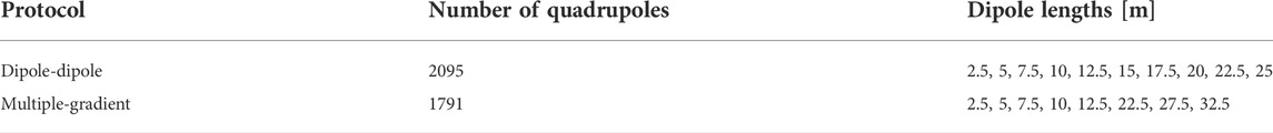
TABLE 1. Characteristics of the used electrode configurations, namely, dipole-dipole combining different dipole lengths and multiple-gradient. For the latter, the dipole lengths refer to the size of potential dipoles nested inside the current dipole.
Processing of the data (i.e., outlier removal) is based on the methodology outlined by Gallistl et al. (2018), that originates from the time-domain IP processing scheme proposed by Flores Orozco et al. (2018b). The fundamental idea is that pseudosections (i.e., a representation of the measured raw data), due to the nature of IP imaging data sets, should reveal spatial consistent patterns, i.e., “smooth” changes in the measured phase-shift φ without the occurrence of large discrepancies or abrupt changes. Those measurements with poor spatial consistency can be considered outliers and should be removed prior to inversion. The processing scheme presented in Gallistl et al. (2018) quantifies this spatial consistency in the phase-shift data by grouping measurements collected with the same current dipole, a subsequent computation of a median phase value for measurements in the corresponding group and the computation of a deviation value ∆φ for each measurement in the group to the median value. Spatial consistent measurements are then defined as those with a small deviation, whereas measurements related to large deviations are considered outliers and are removed.
Inversions of the imaging data sets were performed with CRTomo (Kemna, 2000), using a robust inversion scheme. Such an approach permits to improve the convergence of the inversion and it is less sensitive to wrong estimates of the data error (LaBrecque and Ward, 1990; Morelli and LaBrecque, 1996; Kemna, 2000). All inversions converged to a root-mean-square error close to 1 and a slightly preferential smoothing in horizontal to vertical direction (10:1) was used. We selected this smoothing factor based on the assumption that deformation of the old slope materials in Zone IV (cf. Figure 1) will follow the uplift pressure of the landslide deposits, resulting in an undulating relief and likely only minor deviations from a horizontal layering. For materials associated to the mudflow in Zone III, intermixing of materials of the Ampflwang, Hausruck and old slope sediments is likely to have occurred. However, we do not believe that the individual layers will deviate much from a horizontal position and a slight smoothing in horizontal direction is justified.
Transient electromagnetic (TEM) soundings were used to gain information about vertical variations of the electrical properties across the study area. Measurements were conducted using a single-loop geometry, where the same cable is used as transmitter and receiver, typically in a closed square or circular geometry. The method is based on the circulation of a direct current in the transmitter loop, which generates a primary magnetic field. The abrupt switch-off of the direct current induces eddy currents into the subsurface. This system of eddy currents decays over time and generates the secondary magnetic field (Ward and Hohmann, 1988). The temporal variations of this secondary magnetic field are measured in the receiver loop in terms of a voltage that is sampled along logarithmically distributed time windows. Since the measured decay of the secondary magnetic field depends on the subsurface electrical resistivity, inverse modelling can be used to reconstruct resistivity changes at depth along 1D profiles below the sounding position (e.g., Christiansen et al. (2006)).
Single-loop TEM data was collected along 16 profiles for a total of 517 soundings between the 1st and 4th June in 2018 using a TEM-FAST 48 manufactured by AEMR (Applied Electromagnetic Research). We used a circular loop with a radius of approx. 4 m for a cable length of 25 m (i.e., transferring to a square loop of 6.25 m side length) and a 12 V power source with a 1 A direct current, corresponding to a magnetic momentum of 39 Am2, to collect the data. The voltage decay was sampled along 24 time windows up to 256 µs after current shut-off and we used a total stacking of 9,984 transients to increase the signal to noise ratio. The average sounding spacing was about 8 m except for the southern part of the study area where overlapping measurements were performed (i.e., a loop center separation of 4 m; cf. Table 2 and Figure 2B). The location of each sounding was determined with an RTK-GNSS.
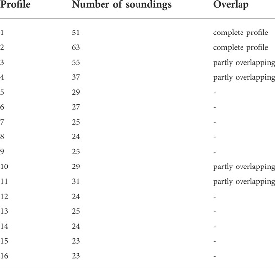
TABLE 2. Number of TEM soundings in each profile (with profile 1 starting in the south) and indication if overlapping measurements were performed (i.e., subsequent TEM loops overlap).
Preprocessing of the TEM data consisted of a visual inspection of the TEM soundings and a manual removal of erroneous voltage readings, i.e., readings that deviate from the expected smooth decay or negative voltage readings. Early-time readings up to 25 µs were particularly affected by noise likely related to an enhanced turn-off ramp effect caused by a highly conductive (< 0.5 Ω) loop cable (Aigner et al., 2021). Therefore, the first 10 time gates of each sounding were removed from the entire data set. Furthermore, we filtered additional readings in the late-times depending on the observed curve smoothness and the presence of negative voltage readings. 1D sections of the vertical changes of electrical resistivity were obtained by inverting the data with ZondTEM1D (Kaminsky, 2001) using a smoothness-constraint regularization. To permit a fair discretization over the entire model depth, a model with 16 layers with fixed thickness was chosen. Using a number of layers in the model much larger than the actual number of lithological layers observed in the boreholes permits a fair discretization in the inversion. We then evaluated the data fit and removed additional voltage readings where the measured data was not fitted by the inverted model.
The refraction seismic method (RST) is based on the propagation and refraction of artificially generated seismic waves in the subsurface and the measurement of ground motion in order to measure travel times of the refracted waves between the shot point and geophone locations. Such travel times can then be inverted to construct a continuous model of the subsurface velocity of P-waves, which depends on the density and the elastic properties of the material (Lankston, 1990). Contrasts in P-wave velocity can be used to infer the contact between unconsolidated sediments and the bedrock. (Leucci et al., 2007; Parasnis, 2012).
To support the interpretation of the electrical results, 10 RST profiles (Figure 2C) were measured between 12th to 16th June in 2017 and between 23rd to 26th April in 2019. Summit seismic recorders (by DMT, Germany) with 24 channels were used to record the seismic wave-field. For our surveys we deployed 30 Hz vertical geophones and collected 1,024 ms traces with a sampling of 1/4 ms. A 5 kg sledgehammer was used as a seismic source and a stack of three shots was made at each geophone location. Table 3 presents the orientation of each profile, as well as the corresponding number of geophones and geophone spacing. The signal processing, consisting of a low-pass filter and an amplitude amplification, and the first break picking were performed with code developed by M. Steiner at the TU Wien. The refraction module of pyGIMLi (Rücker et al., 2017) was subsequently used to invert the travel times to recover 2D sections of seismic velocity using a smoothness-constraint inversion scheme.
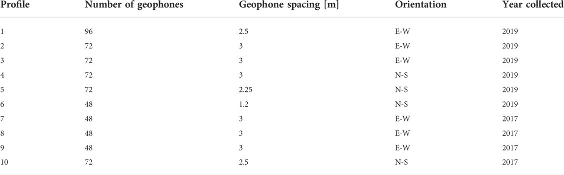
TABLE 3. Number of deployed geophones, the geophone spacing, the orientation and year of collection of the seismic profile.
In April of 2017, five boreholes were drilled across the study area (Figure 2D) in depths varying between 16 and 30 m (cf. Table 4). For each borehole, coring was performed with a diameter of 180 mm and the retrieved sediments were stored for subsequent laboratory analysis and geological description. The lithological composition of the boreholes was similar and featured sediments of the Hausruck, Ampflwang and Ottnang formation and materials of the first two formations were found to be variably disturbed and mixed due to past landslide processes.

TABLE 4. Drilled depth, performed laboratory investigations and associated number of samples in each borehole. The mineralogical investigations included both bulk rock and clay mineralogy.
After the drilling of the boreholes, electromagnetic well-log measurements were conducted at each location using a Dual Induction Probe (by Robertson Geologging Ltd., UK), including continuous logs of the natural gamma radiation and apparent conductivity (Spies, 1996). Gamma logging is a widely used methodology to investigate formations (Schnyder et al., 2006) as specific minerals and sediments, such as feldspar, clays and shales host a larger number of radionuclides (Thorium, Potassium and Uranium) that emit gamma rays. Hence, gamma logs were used here to aid in the interpretation of clay-rich layers. Yet, the occurrence of organic matter might impose limitations on its interpretation (Myers and Wignall, 1987).
In total, 43 samples of the predominant layers within the core were probed and analyzed at the Geological Survey of Austria. The analysis included: 1) bulk rock mineralogy and clay mineralogy (< 2 µm fraction) determined by XRD (PANalytical X’Pert Pro Powder), 2) grain size distribution based on a combined analysis of wet sieving and Sedigraph (< 0.032 mm), and 3) cation exchange capacity (CEC) together with a chemical analysis of major and trace elements. CEC was determined with the barium chloride method (ÖNORM L 1086–1). Moreover, 11 samples were tested on their liquid and plastic limits at a certified testing laboratory (TPA, Vienna). Table 4 presents the number of samples and their distribution for each borehole.
Figure 3A presents the CC imaging results for the profile WD2 (cf. Figure 2A) expressed in terms of the real
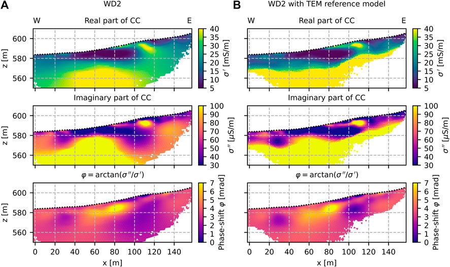
FIGURE 3. Complex conductivity imaging results for the profile WD2 expressed in terms of the real
Figure 4B presents the inverted TEM models collected along the same profile. The TEM models indicate practically only two layers: a shallow one with resistivity values larger than 20 Ωm and a thickness of 5–10 m, whereas a low resistivity layer (ρTEM < 8 Ωm) can be found below it. Compared to the CCI images, the TEM results provide an increased contrast at depths larger than 12 m and at the edges of the CCI profile. The contact to materials with high electrical conductivity (and therefore low resistivity) cannot be resolved with a standard inversion of the CCI data, which favors smooth variations in both lateral and vertical direction.
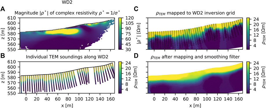
FIGURE 4. (A) Electrical imaging results for the profile WD2 expressed in terms of the magnitude |ρ∗| of the complex resistivity ρ∗ = 1/σ∗, as well as (B) the inverted TEM data collected along the same profile. (C) shows TEM resistivity values ρTEM mapped to the inversion grid of WD2 using nearest neighbor interpolation and (D) the same section after applying a smoothing filter.
TEM inversion results have been used to support the interpretation of ERT and to a lesser extent CCI, for instance to delineate regional aquifer geometry (Meier et al., 2014), to trace saline contamination due to coastal salt water intrusion (Balia and Viezzoli, 2015; Ardali et al., 2018) and to investigate karst lakes (Bücker et al., 2021). Caterina et al. (2014) have shown that the incorporation of prior information in the inversion can help to obtain a more geologically plausible subsurface model. This can be achieved by modifying the regularization operator to account for a reference model (e.g., Oldenburg and Li, 1994) and was done for example by Catt et al. (2009) using EM data from a ground conductivity meter. Hence, we use the inverted TEM model as a reference model for the inversion of the CCI data in order to enhance the horizontal layering and to improve the vertical contrast between the electrical units. Other studies have proposed a joint inversion, where ERT and TEM data are solved simultaneously for the same resistivity model (e.g., Martinez-Moreno et al., 2017; Christensen 2022). However, the inclusion of CCI data in such scheme is beyond the scope of this manuscript.
For the construction of the TEM reference model, in a first step, we selected those TEM soundings that are located along to the CCI profiles. We note here that the inverted 1D TEM resistivity models are always considered to be perpendicular to ground surface; thus, these are tilted to account for the topography changes and mapped to the inversion mesh using nearest neighbor interpolation. Yet, due to the nature of the nearest neighbor interpolation, the so obtained models are not smooth (Figure 4C) and would likely lead to implausible inversion results. Hence, we perform a topography constrained bounding box to smooth the TEM models. Accordingly, for each model cell, we define a rectangular bounding box with given x- and z-axis lengths (32 and 12 m; i.e., 2.6:1 smoothing) which is then rotated based on the slope of the topography. After that, the median value of all model cells inside the bounding box is computed and reassigned to a second mesh. We use a second mesh for the reassignment to avoid mutual dependencies of the smoothing outcome due to the sequence of model cells selected. Figure 4D presents the final reference model after mapping of the TEM values and the smoothing procedure revealing a “smooth” resistivity model.
The resistivity models from CCI and TEM are consistent, as observed in Figure 4A and Figure 4B, thus permitting to incorporate the electrical layer distribution computed for the TEM data (Figure 4C) as described above. Following this approach, we obtain the model presented in Figure 4D. The comparison of the models in Figure 4A and Figure 4D shows consistent models with variations in the magnitude of the electrical resistivity values. Such discrepancy is related to the different volumes for each measurement (i.e., quadrupoles with an electrode separation of 2.5 m when compared with a transmitter loop with an area of 39 m2, e.g., Auken et al., 2006). To overcome this, we scaled the resistivity values retrieved from the inversion of TEM data by the computation of a transfer function. In detail, we extracted the |ρ∗| values from the inverted CC imaging section at the location of the tilted TEM soundings, and computed a linear regression as presented in Figure 5. We used individual transfer functions for each electrical profile. Furthermore, we investigated the use of the reference model without a rescaling of the resistivity values, which revealed only minimal changes in the solved images compared to the rescaled ones, as expected, considering that during the inversion the actual resistivity values are fitted to the measured data and the reference model only aids within the regularization (Caterina et al., 2014). Hereafter, we refer only to CCI results obtained using a reference model in the inversion based on the rescaled TEM model. We note here that we used a homogeneous half space with φ = 0 for the impedance phase of the reference model. In Figure 3B, we present the CCI images for the profile WD2 after inversion with the TEM reference model. As it can be seen in Figure 3B (bottom row), the use of a homogeneous reference model for the phase-shift has only minor effects on the obtained phase-shift image. A comparison with Figure 3A also shows that small scale lateral changes in shallow depths (e.g., the polarizable anomaly, with
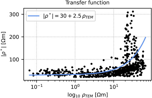
FIGURE 5. Linear transfer function used to scale ρTEM to fit the order of magnitude of |ρ∗| observed in the electrical imaging.
We present in Figure 6 the seismic P-wave velocity and improved CC imaging results for profiles located at the southern border, in the center and at the northern border of the study area (Figure 2). Moreover, to evaluate the seismic and electrical response in comparison to actual soil-physical properties, we present lithological logs overlapping the seismic and CC imaging results. The lithological logs correspond to the soil textural analysis of subsurface materials recovered during the drilling of the boreholes WUR02 and WUR03 collocated to the profile WD13 and borehole WUR04 collocated to profile WD2.

FIGURE 6. (A,B) Complex conductivity imaging results expressed in terms of the real
Images of the real conductivity
To facilitate the comparison between the CCI and RST results, the interface between the two electrical units in the
The layered model interpreted from both the
We observe a fair qualitative agreement between borehole information and the inverted electrical data. Hence, in a first step, we extracted the model parameters from the electrical images at the depth and location of the boreholes. The extracted model parameters are computed as the median value of a k-nearest neighbor search (with k being five elements of the electrical model) and the starting point for the search being the depth and location of the borehole relative to the profile. In a second step, we correlated the available soil-physical and extracted electrical model parameters. For this analysis, we only used borehole data from the wells WUR01, WUR02, WUR03 and WUR05, while the information corresponding to well WUR04 will be used in a later step to evaluate the retrieved petrophysical models. For the sake of brevity, we only present the most significant correlations that are later on discussed in the upscaling approach.
Our analysis revealed that the most significant correlations were observed between the grain size distribution (i.e., the different soil volume fractions of gravel fg, sand fsa, silt fsi and clay fc) and the polarization response expressed in terms of the imaginary component of the complex conductivity
and fits our data to a reasonable R2 score of 0.71. The

FIGURE 7. Scatter plots of the imaginary conductivity
Finally,
The correlation of
Implicitly, this approach also ensures that the total fraction is always capped at 100%. Figure 8 presents the shape of the prediction functions for fg, fsi, fc, as well as fsa as a loss function. In general, we predict coarser textures (sand and gravel) for
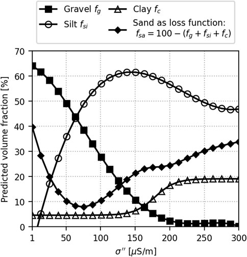
FIGURE 8. Shape of the modelled functions used to predict the different soil fractions for gravel fg, sand fsa, silt fsi and clay fc based on their dependence on
Given the relationships that link the imaginary conductivity to soil fractions, we now have a practical tool to upscale from borehole information (i.e., retrieved samples from drilling) to spatially continuous information over the entire study area. In Figure 9, we use the Equations (6)-(9) for the estimation of gravel, silt, clay and sand from the electrical imaging results from profile WD13 across the entire imaging plane. Based on the soil classification system (NRCS, 1993 - from the United States Department of Agriculture, USDA), we include a classification of soil texture in Figure 9, as well as the soil texture reported from the core analysis of the boreholes WUR02, WUR03 and WUR05.

FIGURE 9. Predicted fractions of (A) gravel (fg), (B) sand (fsa), (C) silt (fsi) and (D) clay (fc) for the profile WD13 and (E) the corresponding predicted soil texture with ground-truth information from boreholes WUR02, WUR03 and WUR05 superimposed over each section.
The comparison of borehole and electrical data reveals a good agreement between the predicted and reported soil textures, with exception of the deep fine-grained units in WUR03. For the hydrogeological interpretation of our results, we now define two main units. A top layer, from the surface to a depth varying between 12 and 18 m, which consists of sandy gravels intercalated by peat, loam and silt loam. Below there is a bottom layer, characterized mostly by fine-grained sediments. Such bottom layer consists of a thin clay unit on top of loam and silt loam. In terms of the stratigraphy, the top layer can be related to the Hausruck formation, whereas the bottom layer corresponds to the Ampflwang and Ottnang formation respectively. Albeit mixtures of different formations, due to past landslide events, can be expected in both layers.
Soil hydraulic properties are preferred over soil texture alone as it provides direct information about water flow. Hence, in a second step, we investigate the possibility to retrieve hydraulic conductivity estimates in an imaging framework built on the quantitative correlation of geophysical and borehole data. We used the recent adaption of Rosetta (Zhang and Schaap, 2017) to estimate Ks (along with the VG parameters) from our predicted soil fractions. As Rosetta uses the volume fractions of sand, silt and clay as input with the requirement that the fractions sum up to 100% soil volume, we had to modify our sand prediction function. Accordingly, our sand prediction (
In particular, Eq. (10) predicts larger fractions of sand for
Figure 10 presents the resulting Ks distribution for WD13 applying Rosetta to our data. For completeness, the VG parameters as well as the soil texture classification when using the adapted sand computation are presented in the (Figure A1). In general, the predicted Ks values are roughly distributed over two orders of magnitude (4.0 × 10⁻⁶ to 1.0 × 10⁻⁵ m/s) with largest values observed for gravelly textures in the top layer, e.g., at the location of WUR02 and WUR05. At depth, the model predicts the lowest Ks values (Ks < 4.0 × 10⁻⁶ m/s) that seem to trace the layers of clay, loam and silt loam in WUR02 and WUR05.
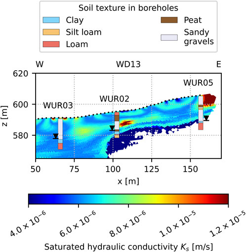
FIGURE 10. Predicted saturated hydraulic conductivity Ks for the profile WD13 using the Rosetta PTF (Zhang and Schaap, 2017), which uses the volume fractions of sand, silt and clay as input parameters. To aid the interpretation of the Ks patterns, the soil texture observed in the boreholes WUR02, WUR03 and WUR05 is also presented. The reversed black triangles indicate the water tables reported during drilling.
WUR03 shows only moderate Ks values (6.0 × 10⁻⁶ m/s). As depicted in Figure A1, the overall texture in WD13 is dominated by loamy components (silt loam and sandy loam), which is also reflected in the predicted homogeneous Ks values. In this context, both lateral and vertical variations, e.g., at WUR02, can be explained by either a higher portion of sand that leads to an increase of Ks > 8.0 × 10⁻⁶ m/s, or larger fractions of silt corresponding to a decrease in Ks < 7.0 × 10⁻⁶ m/s.
Considering the implications of the Ks prediction on the slope hydrogeology, the bottom layer with Ks values below 4.0 × 10⁻⁶ m/s is expected to act as hydraulic barrier for interflow, whereas the top layer can be considered as an unconfined aquifer that permits infiltration of surface water. This interpretation is supported by water tables reported during drilling, which were found at the depth of the clay layer or slightly above it (as depicted in Figure 10). Interflow along the interface between bottom and top layer will likely result in weathering of slope materials (i.e., the dissolution and accumulation of fine grains) and, therefore, development of weathered loam.
We have shown that for WD13 the hydrogeological system is governed by practically two layers: an unconfined aquifer with a thickness of 12–18 m on top of a unit with low hydraulic conductivity. Hence, in a next step we investigated how the interface topography changes for the entire study area, as well as the possibility to delineate possible preferential water-flow paths based on a combined interpretation of the interface topography and the geomorphological surface features.
The comparison of Figure 6 and Figure 10 clearly shows that the transition from low to high
Figure 11 shows the so obtained aquiclude interface for the entire study area as well as the DEM hillshade with a color-coded surface elevation overlay. Furthermore, to aid the interpretation of the topographical changes of the aquiclude interface, the gradient vector magnitude in each grid cell is also presented. In general, the interface reveals a decrease in the elevation from east to west consistent to the surface elevation. However, clear differences can be observed in the eastern part of the study area (X > 25,050 m) where the interface reveals a much steeper dipping (i.e., densely grouped isolines) compared to surface topography.
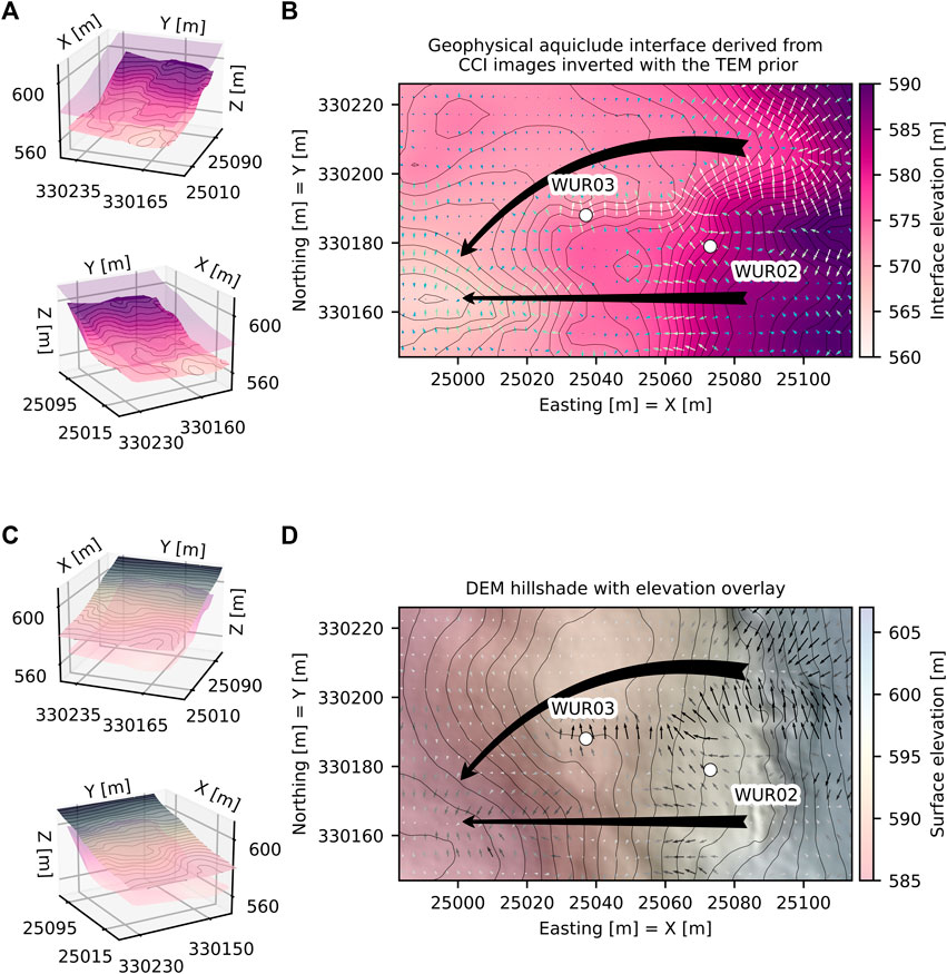
FIGURE 11. Aquiclude interface derived from combination of CCI (using the TEM reference model) and RST in (A) 3D representation (grey shading indicates the DEM) and (B) as map with the corresponding gradient vector magnitudes (small regularly distributed and color-coded arrows) and interpreted preferential water-flow paths (black arrows) superimposed on it. (C) and (D) present the corresponding 3D view and map of the color-coded surface topography, again superimposing both the gradient vectors magnitudes and preferential flow paths from the aquiclude map.
In a similar manner, the surface topography shows a bulge north-west of WUR03; whereas the interface topography indicates a depression. Based on the isolines and gradient magnitudes of the interface layer, we propose two possible preferential water-flow paths, as depicted in Figure 11. In particular, Figure 11 shows 1) a channel starting in the north-eastern part of the study area and continuing north of WUR03 to the south-western part of the study area; and, 2) a roughly direct channel from the south-eastern to the south-western part of the study area. The pathway 1) can clearly be traced by the form of the isolines and gradient vector magnitudes which indicate a depression and likely channeling of interflow, while for pathway 2) a small bulge for the eastern part (X > 25,060 m) and a more pronounced depression of the western part (X < 25,040 m) can be observed. Both 1) and 2) seem to merge in a common location (roughly at X=24,990 m, Y=330,165 m).
Figure 11 indicates that the largest surface topographical changes are associated to those locations where the topography of the interface exhibits the largest gradient vector magnitudes, particularly visible in the eastern part of the study area. We argue that the channeling of interflow through preferential flow paths will likely accelerate weathering or changes in pore-pressure and, therefore, could promote subsidence in those particular areas. Following this argumentation, the bulge in the surface topography north-west of WUR03 is interpreted as deformation of the plastic-reacting slope sediments or materials of a former mudflow as a reaction of the uplift pressure of the main landslide (cf. Figure 1C). To attenuate this effect, a possible counter-measure could include extending the drainage system downslope below the former source/waterlogged area. This could mitigate the channeling of subsurface water-flow along the interface topography.
Figure 9 and Figure 10 demonstrate the ability of the geophysical data to recover subsurface heterogeneity regarding the variations in textural parameters. We propose the combination of geophysical data with Rosetta for the estimation of subsurface hydraulic conductivity in an imaging framework. However, to properly evaluate the accuracy of our approach, it is necessary to compare the estimated values with independent data. To this end, we evaluate here the textural parameters estimated at the position of the borehole WUR04, where ground-truth data is available but was not used for the calibration of petrophysical parameters conducted above.
Figure 12 shows the complex conductivity and seismic velocity extracted from the inversion results (obtained for WD4 and WS1) and the predicted soil fractions at the location of WUR04 as well as borehole data (grain size of recovered samples, natural gamma radiation and conductivity logging). The geophysical data was obtained from an extraction box with a width of 1.5 m. For the prediction of textural parameters, we computed the moving average of the quadrature 1D profile (

FIGURE 12. Comparison of ground-truth information, complex conductivity response and predicted parameters: (A) complex conductivity response in terms of real
For the predicted soil fractions, we observe a good agreement for the gravels, especially at the depth of 7.5 m, where both the predicted and the measured grain size indicate a fraction of gravel of 50%, with the content of coarse materials decreasing at 12.5 m depth, and becomes negligible at a depth of 16 m. The predicted fraction of silt below 12.5 m depth is in line with the measured values in soil samples; however, our model appears to slightly overestimate the silt content (approx. 10%) for the sandy gravels at 7.5 m depth. Accordingly, our model predicts ca. 10% less sand content for the layer at 7.5 m depth. The prediction of clay content reveals a constant value of 5% from the surface to a depth of ∼13 m, where it increases to a value of 20%, which is in agreement with the values reported from the analysis of samples. However, the clay-rich layer (clay > 85%) at 4.5 m is not resolved in our prediction. As previously mentioned, in our correlation function (Equation (8)) we decided to exclude large clay fractions related to kaolinite, as they seem to be clustered in a single location. Accordingly, our approach is not able to predict clay fractions larger than 20%. Considering that such high clay contents are only rarely observed, the approach proposed represents the best compromise to simplify our model linking the polarization response (
The predicted Ks profile presented in Figure 13 shows intermediate values (Ks ∼ 5.0 x 10⁻⁶ m/s) between (roughly) 0.5 and 4 m depth, where the seismic velocity data shows maximum values around 700 m/s corresponding to a coal-bearing clay layer occurring at this depth. The velocity maximum likely indicates a higher degree of compaction for the clay layer, in turn explaining the low hydraulic conductivity values resolved. Below 4 m depth, our prediction shows the largest values (Ks > 5.0 x 10⁻⁶ m/s) associated to sandy gravels (gravel fraction 50%) down to a depth of 12 m and a smooth transition to slightly lower values (Ks < 2.0 x 10⁻⁶ m/s) for the silt layer (with a combined clay and silt content above 75%) below 12 m depth. Moreover, below 12 m depth the seismic velocity increases from 600 m/s to 1,000 m/s, which indicates an increase in compaction, in agreement with the estimated Ks values. Between 10 and 12.5 m depth, the estimated Ks indicates a slight decrease that could be related to a clay-rich lens. Although no analysis was conducted on samples of this particular location, the natural gamma indicates a significant spike at this depth, similar to the one associated to the coal-bearing clay layer mentioned above, therefore sustaining the resolved change in the Ks values.
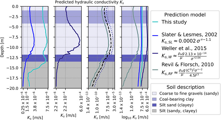
FIGURE 13. Predicted hydraulic conductivity Ks using our approach (cyan) and the relationships by Slater and Lesmes (2002) (blue), Weller et al. (2015) (dark blue) and Revil and Florsch (2010). The dotted, dashed and solid line refer to formation factors computed for fluid conductivity values of 19, 35, and 60 mS/m. The color-coded backgrounds indicate the textural units.
Besides the evaluation of our estimations with independent data from borehole WUR04, we also compare our estimated Ks prediction with hydraulic conductivity values computed using existing
In their study, Weller et al. (2015) investigated 38 unconsolidated soil samples, demonstrating an inversely linear correlation between
In this study we used a dynamic viscosity (µ = 0.0010518) and density (ρ = 998.59) for water at 18°C and an acceleration due to gravity (g = 9.8073) to transform the permeability values k* to hydraulic conductivity values Ks,W. For the sake of completeness, we also computed the hydraulic conductivity values using the model by Revil and Florsch (2010), which also links the imaginary component
in which CS is the specific conductance of the Stern Layer assumed equal to 4 x 10⁻⁹ and F the electrical formation factor describing the ratio between tortuosity and porosity (Katz and Thompson, 1987). Following the approach by Weller et al. (2010), we used a first order approximation for the computation of F based on the ratio of the bulk conductivity (σ0) to fluid conductivity (σw), such as
In our case, σ0 was given by the real component of the complex conductivity (
Ks,SL estimates are consistent to those predicted by our approach; however, Ks,SL values fluctuate around 1.0 × 10⁻⁶ m/s, representing one order of magnitude smaller than our predictions. Actually, vertical variations of the Ks,SL values are identical down to a depth of 10 m, for the unconsolidated materials with coarse grains. At this depth Ks,SL monotonously decreases with depth; whereas our prediction shows two peaks, one related to high hydraulic conductivity values (between ∼12 and 14 m depth) and the lowest values resolved between 16 and 17.5 m depth corresponding to the clayey silt layer. Since the Ks,SL estimation is a direct function of
The use of the model proposed by Weller et al. (2015) shows a larger range of hydraulic conductivity values (between 2.2 x 10⁻⁶ and 6.0 x 10⁻⁴ m/s). However, such variability cannot easily be understood in the study area, where high contents of fine grains are also observed in the top layer. Moreover, the Ks,W cannot resolve for the increase in the hydraulic conductivity resolved at the contact between the silt sand and the silt (ca. 13 m depth). Similar to the approach by Slater and Lesmes (2002), the model by Weller et al. (2015) is only related to the changes in the polarization (
Albeit the discrepancies observed in Figure 13, the three methods (Slater and Lesmes (2002); Weller et al. (2015) and our approach) solve for the same maximum between 7.5 and 10 m depth, which corresponds to the gravels and the low polarization response. For the sake of completeness, we also present estimated values using the model proposed by Revil and Florsch (2010) based on the polarization of the Stern layer. Such model results in hydraulic conductivity values much lower than the rest of the predictions. Such discrepancy may be explained by the rough estimation of the formation factor due to the lack of more detailed information. It seems that the crude approximation, based on the ratio of the fluid-to-bulk conductivity (Equation 14), fails to solve for adequate F values, resulting in inaccurate estimations of the hydraulic conductivity. In this regard, the use of equations with less parameters (e.g., the one by Slater and Lesmes, 2002) provides clear advantages for field investigations. Accordingly, our approach permits to estimate hydraulic conductivity based solely on geophysical data and grain size analysis, which is one of the common measurements in landslide investigations. Further methods requiring of measures of the formation factor, or other parameters may be limited to areas where such information is available.
As previously stated, Rosetta can only be applied to SSC data and therefore the initial set-up did no incorporate training data containing gravel fractions. Further studies may investigate the use of more complex PTFs that permit the incorporation of the gravel fraction. However, originating from soil science, most readily available PTFs are restricted to SSC only (Van Looy et al., 2017). Hence, we believe that our approach offers a flexible tool able to quantify hydraulic conductivity variations at the field-scale based on complex conductivity imaging results. It is important to note that the use of the complex conductivity permits to explicitly take the surface conductivity into account, which may explain high conductivity values in clayey areas. Hydraulic estimations based only on real-valued electrical resistivity, may fail to account for surface conductivity, misinterpreting clay rich formations as areas with high water content. The application of the two-step approach proposed here (first the soil fraction and only then the Ks values) seems to account for existing ground truth data, for subsurface heterogeneity as well as variations in the geophysical properties (complex conductivity and to certain extent seismic velocities). Therefore, our approach may represent a step forward in the upscaling of the relationship between
We have shown that complex conductivity imaging permits to solve for changes in electrical properties consistent with lithological contacts recovered from boreholes. The lithological units resolved in our study correspond to, from top to bottom: a layer with moderate conductivity values (5 >
We present a quantitative interpretation of the complex conductivity images, using both soil-textural data and well-logging information. Within this study we derive site-specific petrophysical relationships that link the imaginary complex conductivity to the fractions of gravel, silt and clay. These well-determined relationships–with R2 scores of 0.71 for gravel, 0.87 for silt and 0.81 for clay–permitted to estimate the textural properties of the resolved geophysical units, which were found consistent to grain size distribution measured in soil samples recovered from core drilling. The textural information was used in the Rosetta pedo-transfer function to predict Ks from the complex conductivity imaging results. Hence, an estimation of hydraulic conductivity values was obtained for the entire study area.
The application of the two-step approach proposed here (i.e., first the soil fraction and then the Ks values) provides comparable values to those computed using existing petrophysical equations developed from laboratory investigations. Such petrophysical equations consider the polarization response at 1 Hz yet are based on measurements typically performed on small, well sorted samples under fully saturated conditions. Therefore, those equations may be limited in field applications, associated to large degrees of heterogeneity and variations in water content. Hence, the approach proposed here permits to derive Ks based solely on available data, namely complex conductivity and grain size distributions, without the need to upscale petrophysical equations resolved in the laboratory.
The raw data supporting the conclusion of this article will be made available by the authors, without undue reservation.
JG, AF contributed to conception and design of the study. MP, JB organized the soil-physical database. JG, AF, LA performed the processing of the geophysical data. JG wrote the first draft of the manuscript. AF, DS, MP, and LA wrote sections of the manuscript. All authors contributed to manuscript revision, read, and approved the submitted version.
This work is supported through the Austrian Science Fund (FWF)—Agence Nationale de la Recherche (ANR) research project I 2619-N29 and ANR-15-CE04-0009-01 HYDRO-SLIDE: Hydro-geophysical observation for an advanced understanding of clayey landslides.
The authors declare that the research was conducted in the absence of any commercial or financial relationships that could be construed as a potential conflict of interest.
All claims expressed in this article are solely those of the authors and do not necessarily represent those of their affiliated organizations, or those of the publisher, the editors and the reviewers. Any product that may be evaluated in this article, or claim that may be made by its manufacturer, is not guaranteed or endorsed by the publisher.
Aigner, L., Högenauer, P., Bücker, M., and Flores-Orozco, A. (2021). A flexible single loop setup for water-borne transient electromagnetic sounding applications. Sensors 21 (19), 6624. doi:10.3390/s21196624
Alvioli, M., Melillo, M., Guzzetti, F., Rossi, M., Palazzi, E., von Hardenberg, J., et al. (2018). Implications of climate change on landslide hazard in Central Italy. Sci. total Environ. 630, 1528–1543. doi:10.1016/j.scitotenv.2018.02.315
Ardali, A., S., Tezkan, B., and Gürer, A. (2018). On the salt water intrusion into the durusu lake, istanbul: A joint central loop TEM and multi-electrode ERT field survey. Pure Appl. Geophys. 175 (8), 3037–3050. doi:10.1007/s00024-018-1813-1
Auken, E., Pellerin, L., Christensen, N. B., and Sørensen, K. (2006). A survey of current trends in near-surface electrical and electromagnetic methods. Geophysics 71 (5), G249–G260. doi:10.1190/1.2335575
Balia, R., and Viezzoli, A. (2015). Integrated interpretation of IP and TEM data for salinity monitoring of aquifers and soil in the coastal area of Muravera (Sardinia, Italy). Boll. Geofis. Teor. Appl. 56, 31. doi:10.4430/bgta0136
Balting, D. F., AghaKouchak, A., Lohmann, G., and Ionita, M. (2021). Northern Hemisphere drought risk in a warming climate. npj Clim. Atmos. Sci. 4 (1), 61–13. doi:10.1038/s41612-021-00218-2
Ban, N., Schmidli, J., and Schär, C. (2015). Heavy precipitation in a changing climate: Does short‐term summer precipitation increase faster? Geophys. Res. Lett. 42 (4), 1165–1172. doi:10.1002/2014gl062588
Baumann, S., Robl, J., Prasicek, G., Salcher, B., and Keil, M. (2018). The effects of lithology and base level on topography in the northern alpine foreland. Geomorphology 313, 13–26. doi:10.1016/j.geomorph.2018.04.006
Berg, A., Sheffield, J., and Milly, P. C. (2017). Divergent surface and total soil moisture projections under global warming. Geophys. Res. Lett. 44 (1), 236–244. doi:10.1002/2016gl071921
Binley, A., Hubbard, S. S., Huisman, J. A., Revil, A., Robinson, D. A., Singha, K., et al. (2015). The emergence of hydrogeophysics for improved understanding of subsurface processes over multiple scales. Water Resour. Res. 51 (6), 3837–3866. doi:10.1002/2015wr017016
Binley, A., Keery, J., Slater, L., Barrash, W., and Cardiff, M. (2016). The hydrogeologic information in cross-borehole complex conductivity data from an unconsolidated conglomeratic sedimentary aquifer. Geophysics 81 (6), E409–E421. doi:10.1190/geo2015-0608.1
Binley, A., and Kemna, A. (2005). “Dc resistivity and induced polarization methods,” in Hydrogeophysics (Springer), 129–156.
Binley, A., and Slater, L. (2020). Resistivity and induced polarization: Theory and applications to the near-surface earth. Cambridge University Press.
Blume, T., and Van Meerveld, H. J. (2015). From hillslope to stream: Methods to investigate subsurface connectivity. WIREs Water 2 (3), 177–198. doi:10.1002/wat2.1071
Bogaard, T. A., and Greco, R. (2016). Landslide hydrology: From hydrology to pore pressure. WIREs Water 3 (3), 439–459. doi:10.1002/wat2.1126
Bücker, M., Flores Orozco, A., and Kemna, A. (2018). Electrochemical polarization around metallic particles — Part 1: The role of diffuse-layer and volume-diffusion relaxation. Geophysics 83 (4), E203–E217. doi:10.1190/geo2017-0401.1
Bücker, M., Flores Orozco, A., Undorf, S., and Kemna, A. (2019a). On the role of stern-and diffuse-layer polarization mechanisms in porous media. J. Geophys. Res. Solid Earth 124 (6), 5656–5677. doi:10.1029/2019jb017679
Bücker, M., Undorf, S., Flores Orozco, A., and Kemna, A. (2019b). Electrochemical polarization around metallic particles—Part 2: The role of diffuse surface charge. Geophysics 84 (2), E57–E73. doi:10.1190/geo2018-0150.1
Bücker, M., Flores Orozco, A., Gallistl, J., Steiner, M., Aigner, L., Hoppenbrock, J., et al. (2021). Integrated land and water-borne geophysical surveys shed light on the sudden drying of large karst lakes in southern Mexico. Solid earth. 12 (2), 439–461. doi:10.5194/se-12-439-2021
Campbell, R. H. (1975). Soil slips, debris flows, and rainstorms in the santa monica mountains and vicinity, southern California. U.S: Professional Paper. Govt. Print. Off. (USGS Numbered Series no. 851).
Catt, L. M., West, L. J., and Clark, R. A. (2009). The use of reference models from a priori data to guide 2D inversion of electrical resistivity tomography data. Geophys. Prospect. 57 (6), 1035–1048.
Caterina, D., Hermans, T., and Nguyen, F. (2014). Case studies of incorporation of prior information in electrical resistivity tomography: Comparison of different approaches. Near Surf. Geophys. 12 (4), 451–465. doi:10.3997/1873-0604.2013070
Christensen, N. B. (2022). Joint inversion of airborne TEM data and surface geoelectrical data. The Egebjerg case. J. Appl. Geophys. 196, 104511. doi:10.1016/j.jappgeo.2021.104511
Christiansen, A. V., Auken, E., and Sørensen, K. (2006). “The transient electromagnetic method,” in Groundwater geophysics (Springer), 179–225.
Comas, X., and Slater, L. (2004). Low-frequency electrical properties of peat. Water Resour. Res. 40 (12), 3534. doi:10.1029/2004wr003534
Cook, B. I., Mankin, J. S., and Anchukaitis, K. J. (2018). Climate change and drought: From past to future. Curr. Clim. Change Rep. 4 (2), 164–179. doi:10.1007/s40641-018-0093-2
Cosby, B., Hornberger, G., Clapp, R., and Ginn, T. (1984). A statistical exploration of the relationships of soil moisture characteristics to the physical properties of soils. Water Resour. Res. 20 (6), 682–690. doi:10.1029/wr020i006p00682
Cruden, D. M., and Varnes, D. J. (1996). “Landslide types and processes,” in Landslides: Investigation and mitigation. Editors A. K. Turner, and R. L. Schuster (Transportation Research Board, Special Report 247, National Research Council), 36–75.
Dahlin, T., and Zhou, B. (2006). Multiple-gradient array measurements for multichannel 2d resistivity imaging. Near Surf. Geophys. 4 (2), 113–123. doi:10.3997/1873-0604.2005037
Doetsch, J., Ingeman-Nielsen, T., Christiansen, A. V., Fiandaca, G., Auken, E., and Elberling, B. (2015). Direct current (dc) resistivity and induced polarization (ip) monitoring of active layer dynamics at high temporal resolution. Cold Regions Sci. Technol. 119, 16–28. doi:10.1016/j.coldregions.2015.07.002
Dunn, R. J., Alexander, L. V., Donat, M. G., Zhang, X., Bador, M., Herold, N., et al. (2020). Development of an updated global land in situ‐based data set of temperature and precipitation extremes: HadEX3. J. Geophys. Res. Atmos. 125 (16), e2019JD032263. doi:10.1029/2019jd032263
Flores Orozco, A., Williams, K. H., Long, P. E., Hubbard, S. S., and Kemna, A. (2011). Using complex resistivity imaging to infer biogeochemical processes associated with bioremediation of an uranium-contaminated aquifer. J. Geophys. Res. 116 (G3), G03001. doi:10.1029/2010jg001591
Flores Orozco, A., Bücker, M., Steiner, M., and Malet, J.-P. (2018a). Complex-conductivity imaging for the understanding of landslide architecture. Eng. Geol. 243, 241–252. doi:10.1016/j.enggeo.2018.07.009
Flores Orozco, A., Gallistl, J., Bücker, M., and Williams, K. H. (2018b). Decay curve analysis for data error quantification in time-domain induced polarization imaging. Geophysics 83 (2), E75–E86. doi:10.1190/geo2016-0714.1
Flores Orozco, A., Micic´, V., Bücker, M., Gallistl, J., Hofmann, T., and Nguyen, F. (2019). Complex- conductivity monitoring to delineate aquifer pore clogging during nanoparticles injection. Geophys. J. Int. 218 (3), 1838–1852. doi:10.1093/gji/ggz255
Flores-Orozco, A., Gallistl, J., Steiner, M., Brandstätter, C., and Fellner, J. (2020). Mapping bio- geochemically active zones in landfills with induced polarization imaging: The heferlbach landfill. Waste Manag. 107, 121–132. doi:10.1016/j.wasman.2020.04.001
Flores Orozco, A., Aigner, L., and Gallistl, J. (2021). Investigation of cable effects in spectral induced polarization imaging at the field scale using multicore and coaxial cables. Geophysics 86 (1), E59–E75. doi:10.1190/geo2019-0552.1
Gallistl, J., Weigand, M., Stumvoll, M., Ottowitz, D., Glade, T., and Orozco, A. F. (2018). Delineation of subsurface variability in clay-rich landslides through spectral induced polarization imaging and electromagnetic methods. Eng. Geol. 245, 292–308. doi:10.1016/j.enggeo.2018.09.001
Godio, A., and Bottino, G. (2001). Electrical and electromagnetic investigation for landslide characterisation. Phys. Chem. Earth, Part C Sol. Terr. Planet. Sci. 26 (9), 705–710. doi:10.1016/s1464-1917(01)00070-8
Grandjean, G., Gourry, J.-C., Sanchez, O., Bitri, A., and Garambois, S. (2011). Structural study of the ballandaz landslide (French alps) using geophysical imagery. J. Appl. Geophy. 75 (3), 531–542. doi:10.1016/j.jappgeo.2011.07.008
Grunert, P., Soliman, A., C´oric´, S., Scholger, R., Harzhauser, M., and Piller, W. E. (2010). Stratigraphic re-evaluation of the stratotype for the regional ottnangian stage (central paratethys, middle burdigalian). Newsl. Stratigr. 44 (1), 1–16. doi:10.1127/0078-0421/2010/0001
Hinsch, R. (2008). New insights into the oligocene to miocene geological evolution of the molasse basin of Austria. OIL GAS-EUROPEAN Mag. 34 (3), 138–143.
Holmes, J., Chambers, J., Meldrum, P., Wilkinson, P., Boyd, J., Williamson, P., and Donohue, S. (2020). Four‐dimensional electrical resistivity tomography for continuous, near‐real‐time monitoring of a landslide affecting transport infrastructure in British Columbia, Canada. Near Surf. Geophys. 18, 337–351. Geoelectrical Monitoring.
Huntley, D., Bobrowsky, P., Hendry, M., Macciotta, R., Elwood, D., Sattler, K., et al. (2019). Application of multi-dimensional electrical resistivity tomography datasets to investigate a very slow-moving landslide near Ashcroft, British Columbia, Canada. Landslides 16 (5), 1033–1042. doi:10.1007/s10346-019-01147-1
Jorda, H., Bechtold, M., Jarvis, N., and Koestel, J. (2015). Using boosted regression trees to explore key factors controlling saturated and near-saturated hydraulic conductivity. Eur. J. Soil Sci. 66 (4), 744–756. doi:10.1111/ejss.12249
Katona, T., Gilfedder, B. S., Frei, S., Bücker, M., and Flores-Orozco, A. (2021). High-resolution induced polarization imaging of biogeochemical carbon-turnover hot spots in a peatland. Biogeosciences 2021, 4039–4058. doi:10.5194/bg-18-4039-2021
Katz, A., and Thompson, A. (1987). Prediction of rock electrical conductivity from mercury injection measurements. J. Geophys. Res. 92 (B1), 599–607. doi:10.1029/jb092ib01p00599
Kemna, A., Binley, A., Cassiani, G., Niederleithinger, E., Revil, A., Slater, L., et al. (2012). An overview of the spectral induced polarization method for near-surface applications. Near Surf. Geophys. 10 (6), 453–468. doi:10.3997/1873-0604.2012027
Kemna, A. (2000). Tomographic inversion of complex resistivity: Theory and application. Osnabrück, Germany: Der Andere Verlag.
Konapala, G., Mishra, A. K., Wada, Y., and Mann, M. E. (2020). Climate change will affect global water availability through compounding changes in seasonal precipitation and evaporation. Nat. Commun. 11 (1), 1–10. doi:10.1038/s41467-020-16757-w
Kušnirák, D., Dostál, I., Putiška, R., and Mojzeš, A. (2016). Complex geophysical investigation of the kapušany landslide (eastern Slovakia). Contributions Geophys. Geodesy 46 (2), 111–124. doi:10.1515/congeo-2016-0008
LaBrecque, D. J., and Ward, S. H. (1990). Two-dimensional cross-borehole resistivity model fit ting. Geotechnical Environ. Geophys. 1, 51–57.
Lankston, R. W. (1990). “High-resolution refraction seismic data acquisition and interpretation,” in Geotechnical an environmental geophysics: Volume I: Review and tutorial (Society of Exploration Geophysicists), 45–74. doi:10.1190/1.9781560802785.ch3
Lehmann, P., Merlin, O., Gentine, P., and Or, D. (2018). Soil texture effects on surface resistance to bare‐soil evaporation. Geophys. Res. Lett. 45 (19), 10–398. doi:10.1029/2018gl078803
Leroy, P., and Revil, A. (2009). A mechanistic model for the spectral induced polarization of clay materials. J. Geophys. Res. 114, B10202. doi:10.1029/2008jb006114
Leucci, G., Greco, F., De Giorgi, L., and Mauceri, R. (2007). Three-dimensional image of seismic refraction tomography and electrical resistivity tomography survey in the castle of occhiola (sicily, Italy). J. Archaeol. Sci. 34 (2), 233–242. doi:10.1016/j.jas.2006.04.010
Lévy, L., Gibert, B., Sigmundsson, F., Fóvenz, Ó., Hersir, G. P., Briole, P., et al. (2018). The role of smectites in the electrical conductivity of active hydrothermal systems: electrical properties of core samples from Krafla volcano, Iceland. Geophys. J. Int. 215 (3), 1558–1582.
Li, R., Hu, X., Xu, D., Liu, Y., and Yu, N. (2020). Characterizing the 3d hydrogeological structure of a debris landslide using the transient electromagnetic method. J. Appl. Geophys. 175, 103991. doi:10.1016/j.jappgeo.2020.103991
Lin, Q., Wang, Y., Glade, T., Zhang, J., and Zhang, Y. (2020). Assessing the spatiotemporal impact of climate change on event rainfall characteristics influencing landslide occurrences based on multiple GCM projections in China. Clim. Change 162 (2), 761–779. doi:10.1007/s10584-020-02750-1
Loke, M., Chambers, J., and Ogilvy, R. (2006). Inversion of 2d spectral induced polarization imaging data. Geophys. Prospect. 54 (3), 287–301. doi:10.1111/j.1365-2478.2006.00537.x
Maierhofer, T., Hauck, C., Hilbich, C., Kemna, A., and Flores-Orozco, A. (2022). Spectral induced polarization imaging to investigate an ice-rich mountain permafrost site in Switzerland. The Cryosphere 16(5), 1903–1925..
Martin, T., Günther, T., Flores Orozco, A., and Dahlin, T. (2020). Evaluation of spectral induced polarization field measurements in time and frequency domain. J. Appl. Geophys. 180, 104141. doi:10.1016/j.jappgeo.2020.104141
Martinez-Moreno, F. J., Monteiro-Santos, F. A., Bernardo, I., Farzamian, M., Nascimento, C., Fernandes, J., et al. (2017). Identifying seawater intrusion in coastal areas by means of 1D and quasi-2D joint inversion of TDEM and VES data. J. Hydrology 552, 609–619. doi:10.1016/j.jhydrol.2017.07.026
Meier, P., Kalscheuer, T., Podgorski, J. E., Kgotlhang, L., Green, A., Greenhalgh, S., et al. (2014). Hydrogeophysical investigations in the western and north-central Okavango Delta (Botswana) based on helicopter and ground-based transient electromagnetic data and electrical resistance tomography. Geophysics 79 (5), B201–B211. doi:10.1190/geo2014-0001.1
Morelli, G., and LaBrecque, D. J. (1996). “Robust scheme for ert inverse modeling,” in Symposium on the Application of Geophysics to Engineering and Environmental Problems Proceedings, 629–638. doi:10.4133/1.2922327
Mualem, Y., and Friedman, S. (1991). Theoretical prediction of electrical conductivity in saturated and unsaturated soil. Water Resour. Res. 27 (10), 2771–2777. doi:10.1029/91wr01095
Myers, K. J., and Wignall, P. B. (1987). “Understanding jurassic organic-rich mudrocks—new concepts using gamma-ray spectrometry and palaeoecology: Examples from the kimmeridge clay of dorset and the jet rock of yorkshire,” in Marine clastic sedimentology (Springer), 172–189.
Nemes, A., Rawls, W. J., and Pachepsky, Y. A. (2006). Use of the nonparametric nearest neighbor approach to estimate soil hydraulic properties. Soil Sci. Soc. Am. J. 70 (2), 327–336. doi:10.2136/sssaj2005.0128
Nrcs, U. (1993). “Soil survey division staff (1993) soil survey manual,”. Soil conservation service (US Department of Agriculture Handbook), 18, 315.
Okay, G., Leroy, P., Ghorbani, A., Cosenza, P., Camerlynck, C., Cabrera, J., et al. (2014). Spectral induced polarization of clay-sand mixtures: Experiments and modeling. Geophysics 79 (6), E353–E375. doi:10.1190/geo2013-0347.1
Oldenburg, D. W., and Li, Y. (1994). Inversion of induced polarization data. Geophysics 59 (9), 1327–1341. doi:10.1190/1.1443692
Papalexiou, S. M., and Montanari, A. (2019). Global and regional increase of precipitation extremes under global warming. Water Resour. Res. 55 (6), 4901–4914. doi:10.1029/2018wr024067
Pelton, W. H., Ward, S., Hallof, P., Sill, W., and Nelson, P. H. (1978). Mineral discrimination and removal of inductive coupling with multifrequency ip. Geophysics 43 (3), 588–609. doi:10.1190/1.1440839
Perrone, A., Lapenna, V., and Piscitelli, S. (2014). Electrical resistivity tomography technique for landslide investigation: A review. Earth-Science Rev. 135, 65–82. doi:10.1016/j.earscirev.2014.04.002
Revil, A., and Florsch, N. (2010). Determination of permeability from spectral induced polarization in granular media. Geophys. J. Int. 181 (3), 1480–1498. doi:10.1111/j.1365-246x.2010.04573.x
Revil, A. (2012). Spectral induced polarization of shaly sands: Influence of the electrical double layer. Water Resour. Res. 48 (2). doi:10.1029/2011wr011260
Revil, A., Kessouri, P., and Torres-Verdín, C. (2014). Electrical conductivity, induced polarization, and permeability of the fontainebleau sandstone. Geophysics 79 (5), D301–D318. doi:10.1190/geo2014-0036.1
Revil, A., Florsch, N., and Mao, D. (2015). Induced polarization response of porous media with metallic particles—part 1: A theory for disseminated semiconductors. Geophysics 80 (5), D525–D538. doi:10.1190/geo2014-0577.1
Revil, A., Coperey, A., Shao, Z., Florsch, N., Fabricius, I. L., Deng, Y., et al. (2017). Complex conductivity of soils. Water Resour. Res. 53 (8), 7121–7147. doi:10.1002/2017wr020655
Revil, A., Ahmed, A. S., Coperey, A., Ravanel, L., Sharma, R., and Panwar, N. (2020). Induced polarization as a tool to characterize shallow landslides. J. Hydrology 589, 125369. doi:10.1016/j.jhydrol.2020.125369
Rogers, N. W., and Selby, M. J. (1980). Mechanisms of shallow translational landsliding during summer rainstorms: North Island, New Zealand. Geogr. Ann. Ser. A Phys. Geogr. 62, 11–21. doi:10.2307/520448
Rögl, F. (1997). “Palaeogeographic considerations for mediterranean and paratethys seaways (oligocene to miocene),” in Annalen des Naturhistorischen Museums in Wien. Serie A für Mineralogie und Petrographie, Geologie und Paläontologie, Anthropologie und Prähistorie, 279–310.
Rücker, C., Günther, T., and Wagner, F. M. (2017). pygimli: An open-source library for modelling and inversion in geophysics. Comput. Geosciences 109, 106–123. doi:10.1016/j.cageo.2017.07.011
Rupp, C., Linner, M., and Mandl, W. (2011). Erläuterungen zur geologischen karte von oberösterreich. Vienna: Verlag der Geologischen Bundesanstalt.
Samyn, K., Travelletti, J., Bitri, A., Grandjean, G., and Malet, J.-P. (2012). Characterization of a landslide geometry using 3d seismic refraction traveltime tomography: The la valette land- slide case history. J. Appl. Geophys. 86, 120–132. doi:10.1016/j.jappgeo.2012.07.014
Schaap, M. G., Leij, F. J., and Van Genuchten, M. T. (2001). Rosetta: A computer program for estimating soil hydraulic parameters with hierarchical pedotransfer functions. J. hydrology 251 (3-4), 163–176. doi:10.1016/s0022-1694(01)00466-8
Schnyder, J., Ruffell, A., Deconinck, J.-F., and Baudin, F. (2006). Conjunctive use of spectral gamma-ray logs and clay mineralogy in defining late jurassic–early cretaceous palaeocli- mate change (dorset, u.k.). Palaeogeogr. Palaeoclimatol. Palaeoecol. 229 (4), 303–320. doi:10.1016/j.palaeo.2005.06.027
Searchinger, T. D., Wirsenius, S., Beringer, T., and Dumas, P. (2018). Assessing the efficiency of changes in land use for mitigating climate change. Nature 564 (7735), 249–253. doi:10.1038/s41586-018-0757-z
Sidle, R. C., Greco, R., and Bogaard, T. (2019). Overview of landslide hydrology. Water 11, 148. doi:10.3390/w11010148
Slater, L., Barrash, W., Montrey, J., and Binley, A. (2014). Electrical-hydraulic relationships ob- served for unconsolidated sediments in the presence of a cobble framework. Water Resour. Res. 50 (7), 5721–5742. doi:10.1002/2013wr014631
Slater, L. D., and Reeve, A. (2002). Investigating peatland stratigraphy and hydrogeology using integrated electrical geophysics. Geophysics 67 (2), 365–378. doi:10.1190/1.1468597
Slater, L., and Glaser, D. (2003). Controls on induced polarization in sandy unconsolidated sediments and application to aquifer characterization. Geophysics 68 (5), 1547–1558. doi:10.1190/1.1620628
Slater, L., and Lesmes, D. P. (2002). Electrical-hydraulic relationships observed for unconsolidated sediments. Water Resour. Res. 38 (10), 31-1–31-13. doi:10.1029/2001wr001075
Spies, B. (1996). Electrical and electromagnetic borehole measurements: A review. Surv. Geophys. 17 (4), 517–556. doi:10.1007/bf01901643
Supper, R., Ottowitz, D., Jochum, B., Kim, J.-H., Römer, A., Baron, I., et al. (2014). Geoelectrical monitoring: An innovative method to supplement landslide surveillance and early warning. Near Surf. Geophys. 12 (1), 133–150. doi:10.3997/1873-0604.2013060
Tabari, H. (2020). Climate change impact on flood and extreme precipitation increases with water availability. Sci. Rep. 10 (1), 1–10. doi:10.1038/s41598-020-70816-2
Tarasov, A., and Titov, K. (2007). Relaxation time distribution from time domain induced polarization measurements. Geophys. J. Int. 170 (1), 31–43. doi:10.1111/j.1365-246x.2007.03376.x
Twarakavi, N. K., Simunek, J., and Schaap, M. (2009). Development of pedotransfer functions for estimation of soil hydraulic parameters using support vector machines. Soil Sci. Soc. Am. J. 73 (5), 1443–1452. doi:10.2136/sssaj2008.0021
Uhlemann, S., Hagedorn, S., Dashwood, B., Maurer, H., Gunn, D., Dijkstra, T., et al. (2016). Landslide characterization using p-and s-wave seismic refraction tomography—The importance of elastic moduli. J. Appl. Geophys. 134, 64–76. doi:10.1016/j.jappgeo.2016.08.014
Van Genuchten, M. T. (1980). A closed-form equation for predicting the hydraulic conductivity of unsaturated soils. Soil Sci. Soc. Am. J. 44 (5), 892–898. doi:10.2136/sssaj1980.03615995004400050002x
Van Looy, K., Bouma, J., Herbst, M., Koestel, J., Minasny, B., Mishra, U., et al. (2017). Pedotransfer functions in earth system science: Challenges and perspectives. Rev. Geophys. 55 (4), 1199–1256. doi:10.1002/2017rg000581
Ward, S. H., and Hohmann, G. W. (1988). “Electromagnetic theory for geophysical applications,” in Electromagnetic methods in applied geophysics: Voume 1, theory (Society of Exploration Geophysicists), 130–311. doi:10.1190/1.9781560802631.ch4
Ward, S. H. (1990). Resistivity and induced polarization methods. Geotechnical environ- Ment. Geophys. 1, 147–189. doi:10.1190/1.9781560802785.ch6
Watlet, A., Kaufmann, O., Triantafyllou, A., Poulain, A., Chambers, J. E., Meldrum, P. I., et al. (2018). Imaging groundwater infiltration dynamics in the karst vadose zone with long-term ERT monitoring. Hydrol. Earth Syst. Sci. 22 (2), 1563–1592. doi:10.5194/hess-22-1563-2018
Waxman, M. H., and Smits, L. J. M. (1968). Electrical conductivities in oil-bearing shaly sands. Soc. Petroleum Eng. J. 8 (02), 107–122. doi:10.2118/1863-a
Weiskopf, S. R., Rubenstein, M. A., Crozier, L. G., Gaichas, S., Griffis, R., Halofsky, J. E., et al. (2020). Climate change effects on biodiversity, ecosystems, ecosystem services, and natural resource management in the United States. Sci. Total Environ. 733, 137782. doi:10.1016/j.scitotenv.2020.137782
Weller, A., Nordsiek, S., and Debschütz, W. (2010). Estimating permeability of sandstone samples by nuclear magnetic resonance and spectral-induced polarization. Geophysics 75 (6), E215–E226. doi:10.1190/1.3507304
Weller, A., Slater, L., Binley, A., Nordsiek, S., and Xu, S. (2015). Permeability prediction based on induced polarization: Insights from measurements on sandstone and unconsolidated samples spanning a wide permeability range. Geophysics 80 (2), D161–D173. doi:10.1190/geo2014-0368.1
Weller, A., and Slater, L. (2019). Permeability estimation from induced polarization: An evaluation of geophysical length scales using an effective hydraulic radius concept. Near Surf. Geophys. 17 (6), 581–594. doi:10.1002/nsg.12071
Whiteley, J. S., Watlet, A., Kendall, J. M., and Chambers, J. E. (2021). Brief communication: The role of geophysical imaging in local landslide early warning systems. Nat. Hazards Earth Syst. Sci. 21, 3863–3871. doi:10.5194/nhess-21-3863-2021
Zhang, Y., and Schaap, M. G. (2019). Estimation of saturated hydraulic conductivity with pedo- transfer functions: A review. J. Hydrology 575, 1011–1030. doi:10.1016/j.jhydrol.2019.05.058
Additionally to the saturated hydraulic conductivity Ks the Rosetta PTF (Schaap et al., 2001; Zhang and Schaap, 2017) predicts the parameters of the van Genuchten water retention function (Van Genuchten, 1980):
in which θr (ψ) is the water retention curve in cm3cm−3 as a function of soil water pressure ψ, θr and θs are the residual and saturated water contents in cm3cm−3 and n (dimensionless) and α (1/cm) are curve shape parameters. Figure A1 shows the predicted van Genuchten parameters for the profile WD13 and the soil texture that was used as input for Rosetta.

FIGURE A1. Van Genuchten water retention parameters for the profile WD13 as predicted with Rosetta (Zhang and Schaap, 2017) using the soil texture presented in the bottom subplot. Each subplot further contains the soil texture observed in the boreholes WUR02, WUR03 and WUR05.
Keywords: soil-textural parameters, complex conductivity imaging, hydrogeophysics, induced polarization, transient electromagnetic method, hydraulic conductivity
Citation: Gallistl J, Schwindt D, Birgit J, Aigner L, Peresson M and Flores Orozco A (2022) Quantification of soil textural and hydraulic properties in a complex conductivity imaging framework: Results from the Wolfsegg slope. Front. Earth Sci. 10:911611. doi: 10.3389/feart.2022.911611
Received: 02 April 2022; Accepted: 04 August 2022;
Published: 12 September 2022.
Edited by:
Sebastian Uhlemann, Berkeley Lab (DOE), United StatesReviewed by:
Arkoprovo Biswas, Banaras Hindu University, IndiaCopyright © 2022 Gallistl, Schwindt, Birgit, Aigner, Peresson and Flores Orozco. This is an open-access article distributed under the terms of the Creative Commons Attribution License (CC BY). The use, distribution or reproduction in other forums is permitted, provided the original author(s) and the copyright owner(s) are credited and that the original publication in this journal is cited, in accordance with accepted academic practice. No use, distribution or reproduction is permitted which does not comply with these terms.
*Correspondence: Jakob Gallistl, amFrb2IuZ2FsbGlzdGxAdHV3aWVuLmFjLmF0
Disclaimer: All claims expressed in this article are solely those of the authors and do not necessarily represent those of their affiliated organizations, or those of the publisher, the editors and the reviewers. Any product that may be evaluated in this article or claim that may be made by its manufacturer is not guaranteed or endorsed by the publisher.
Research integrity at Frontiers
Learn more about the work of our research integrity team to safeguard the quality of each article we publish.