Fracture Imaging Using DAS-Recorded Microseismic Events

Staněk, František; Jin, Ge; Simmons, James

doi:10.3389/feart.2022.907749

ORIGINAL RESEARCH article

Front. Earth Sci., 19 July 2022

Sec. Solid Earth Geophysics

Volume 10 - 2022 | https://doi.org/10.3389/feart.2022.907749

This article is part of the Research Topic Advances and Applications of Distributed Optical Fiber Sensing (DOFS) in Multi-scales Geoscience Problems View all 13 articles

Fracture Imaging Using DAS-Recorded Microseismic Events

František Staněk*

Ge Jin

James Simmons

Department of Geophysics, Colorado School of Mines, Golden, CO, United States

Hydraulic fracturing enables hydrocarbon production from unconventional reservoirs. Mapping induced seismicity around newly created fractures is crucial for understanding the reservoir response and increasing the efficiency of operations. Distributed acoustic sensing (DAS) provides a large amount of high spatial resolution microseismic data acquired along the entire length of horizontal wells. We focus on the observed reflected S-waves and develop a new methodology using microseismic events as sources of energy to image induced fractures acting as reflectors in the media surrounding the events and monitoring fiber. The workflow consists of DAS data preprocessing, event location, wavefield separation, raytracing-based imaging, and image post-processing. The comparison of the resulting images with low-frequency DAS signals of fracture hits corroborates that the reflections are from fractures created by stimulation. The proposed algorithm can be used for real-time mapping of fractures and tracking fracture changes in space and time. Fracture imaging leads to a better understanding of the reservoir response to hydraulic fracturing stimulation.

1 Introduction

Microseismic monitoring of hydraulic fracturing has been employed to understand the reservoir response and increase the efficiency of subsurface operations (Grechka and Heigl, 2017). Similarly, induced seismicity monitoring has been used during waste-water injection (e.g., Zoback, 2012), mining (e.g., Mendecki et al., 2010), enhancing geothermal systems (e.g., Kwiatek et al., 2014), storing gas underground (e.g., Carannante et al., 2020), and CO₂ sequestration (e.g., Williams-Stroud et al., 2020) to mitigate seismic hazard.

A commonly provided result of hydraulic fracturing microseismic monitoring is a catalogue of detected microseismic events with their origin time, location of hypocenter, magnitude, and, if possible, a description of source mechanism. The main goals are to describe fracture geometry and orientation, and connectivity between individual fractures and to estimate the area of the rock volume having increased permeability. The interpretation is mostly done with discrete fracture network (Williams-Stroud et al., 2013), stimulated rock volume (Rahimi Zeynal et al., 2014), and geomechanical models (e.g., Staněk and Eisner, 2017). However, due to uncertainties in event locations and inverted fault planes, and a lack of understanding of what microseismicity really represents, more accurate knowledge of induced fracture systems is still in need.

Another technique to map induced fractures, instead of connecting located events, is reflection imaging, using microseismic events as sources of energy. Grechka et al. (2017), Reshetnikov et al. (2010), or Lin and Zhang (2016), observed reflected waves in data acquired by 3C geophone arrays and used them for microseismic imaging. Such imaging is not common, probably because it is difficult to see reflected waves in the microseismic data acquired by sparse and distant geophone arrays.

Recently, distributed fiber-optic sensing technology (Hartog, 2017) providing dense monitoring data has started to be employed as an alternative to the traditional seismic arrays in industry (e.g., Karrenbach et al., 2017; Byerley et al., 2018; Binder and Tura, 2020; Lellouch et al., 2020; Stork et al., 2020; Titov et al., 2021) as well as in global seismology (Zhan, 2019; Lindsey and Martin, 2021). Fiber-optic-based monitoring is a quickly developing technology that has been used for measuring vibrations, temperature, and strain for many different purposes (Baldwin, 2018). Specifically, distributed acoustic sensing (DAS) is being utilized for long-term seismic monitoring. The fiber working as a sensor can be installed along the whole length of the stimulated well (in-well monitoring) or offset wells (cross-well monitoring). The best practice seems to be cementing fiber behind casing for permanent monitoring, although it can also be installed temporarily. Such monitoring geometry allows detection of a high number of weak (i.e., low magnitude) microseismic events due to proximity to the stimulated area. DAS offers other advantages compared to borehole geophone arrays, such as broadband response (from mHz to tens of kHz), long aperture (several km long fiber), and dense spatial sampling (channel spacing can be $<$ 1 m). The main downside of fiber-optic-based monitoring is a single-component axial strain measurement only in the direction along the fiber (Baird et al., 2019). This causes critical problems when locating and inverting the source mechanism of microseismic events detected by a single fiber. However, there are ways to overcome this issue using multi-component, so-called, helical optical fibers (Lim Chen Ning and Sava, 2018), monitoring carried out by a deviated or L-shaped array Verdon et al. (2020), or monitoring with two or more nearby fiber wells (e.g., Cole et al., 2018).

DAS provides high spatial resolution recordings, enabling detailed analyses of wavefields and development of new processing methods, leading to improved interpretations and better insight into the reservoir response. In passive seismic, we rely on induced microseismic events around the monitoring wells at a reasonable distance to detect them. Recorded waves (i.e., arrival times and amplitudes) contain information about event location relative to a monitoring array, radiation pattern due to source processes, and about the media between source and fiber. It also includes the structural features represented by reflected/refracted/diffracted waves arriving later after the direct P-wave arrival (Lellouch and Biondi, 2021). Moreover, in some DAS-based microseismic data, one may observe not only far-field but also near-field signals (Luo et al., 2021a) which can be used for more precise source description, and dispersive guided waves, providing properties of anomalous velocity layers and helping identification of events located inside or outside the reservoir layer (Luo et al., 2021b). While all the phenomena are recorded with high resolution, we can not only map fracture propagation based on microseismic events located along fractures but also image fractures making use of reflected waves.

Another type of fiber-optic-based measurement during hydraulic fracturing used to describe fractures is of low-frequency ( $<$ 1 Hz) DAS (LFDAS). LFDAS measures strain changes (i.e., works as hybrid distributed strain sensing, DSS) induced by hydraulic fractures (Jin and Roy, 2017; Richter et al., 2019; Ugueto et al., 2019; Ichikawa et al., 2020; Zhu and Jin, 2021). The detected strain signals represent fractures which were initiated at the offset treatment well and reached the monitoring fiber well, so-called fracture hits or frac-hits. Therefore, frac-hits are clear proof that the fractures have a half-length longer than the spacing between treatment and monitoring well. Besides the times when fractures hit the monitoring well, LFDAS data also show the time intervals when the fractures open (extension at the fractures and compression zone around) and when they close (extension zone around the fractures) due to the leak-off after injection.

In this study, we analyze selected examples of field DAS-recorded microseismic data acquired during multi-well hydraulic fracturing, focus on observed reflected S-waves, and propose a new method for imaging fractures in the vicinity of induced microseismic events. Imaged fractures are compared to LFDAS frac-hits to corroborate that the imaged waves are reflected from newly created hydraulic fractures.

2 Data and Methodology

2.1 DAS Data and Observations

We analyze data from the Chalk Bluff project in the Denver-Julesburg (DJ) Basin in Colorado, USA. Figure 1 shows a map of the study area with the position of the pad of horizontal wells drilled in a N-S direction through the target unconventional reservoir formations Codell and Niobrara at depths of around 7,400–7,700 ft (TVD). The reservoir was hydraulically fractured in hundreds of stages along the lateral parts of all the horizontal wells. DAS microseismic and LFDAS monitoring of the studied area was carried out by two fibers permanently installed outside the casing of the red wells in Figure 1. The channel spacing was 1 m along the fiber, and the gauge length was set to 5 m.

FIGURE 1

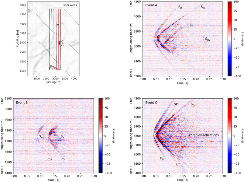
FIGURE 1. Upper left: A map of the studied area with horizontal wells (running N-S) and their relative positions. Wells with permanently installed fiber are shown in red. The diagonal NW-SE wells shown in gray are previously drilled production wells in the Niobrara. The yellow stars represent examples of strong microseismic events (A, B, C). The seismic coherency map in the background may indicate potential faults in the Niobrara formation. Upper right and bottom: Examples of three representative microseismic events with direct P-waves (P_D), direct S-waves (S_D), converted S- to P-waves (SP), and reflected S-waves (S_R) recorded by DAS array. The events A and B are accompanied by other weaker events with very similar moveouts (S_D2, S_R2) indicating similar location but slightly different origin time. Event C shows more complicated reflections after the direct S-wave.

We have analyzed several strong microseismic events visible in the continuous DAS data. The waveforms of most of the events are relatively simple with symmetrical moveouts of direct P- and S-waves, where S-wave signals are usually of higher amplitude than P-waves. In this study, we focus on events that have more complex wavefields, and demonstrate our methodology on three selected example events. DAS data and initial spatial locations (taken from the catalogue of events located from a surface array provided by the data owner) of the three example events are shown in Figure 1 (yellow stars). Events A and C have both clear direct P- and S-waves (marked as P_D, S_D), event B has only an S-wave visible, probably because of the lower magnitude. All three events have reflected S-waves (marked as S_R) but event C has also clearly converted S to P-waves (marked as SP) and a very complex wavefield following the S-wave arrival. We also notice secondary, similarly looking, weaker events coming after and before the main event in the data of the events A and B, respectively (see S_D2, S_R2 in Figure 1). These repeated events most likely occurred at the same locations as the main events but at slightly different times.

The observed reflected waves could represent either a fault, fracture, or velocity interface, acting as a reflector in the medium around the event location at the time when the microseismic event occurred. However, in our case, we can exclude the possibility of reflections from near-horizontal interfaces (i.e., bedding planes) based on travel time moveout. Reflection from a horizontal interface would be recorded by most of the channels along the fiber and be symmetric around the apex with a moveout similar to the direct P- and S-waves. Our observed reflected S-wave moveouts are asymmetrical and parallel to the direct S-wave moveouts. Therefore, we interpret them as reflections from approximately near-vertical faults or near-vertical fractures perpendicular to the horizontal fiber. Furthermore, the reflectors are most probably either very close to or directly intersecting the fiber, as we see that the arrivals of reflected S-waves and direct S-waves merge into the same channels where the reflectors likely intersect with the fiber well.

2.2 Fracture Imaging––Methodology

The reflected S-waves observed in the DAS data indicate the presence of reflectors in the area between the microseismic event locations and the recording fiber. From their moveouts, we may expect that the reflector orientation is near-vertical and perpendicular to the horizontal well. Our first attempt to explain the reflected S-waves was a simple traveltime modeling (Stanek and Jin, 2021). We were able to fit manually picked arrival times of P-, S-, and reflected S-waves sufficiently well with synthetic traveltimes using a homogeneous isotropic velocity model (velocity taken from an available sonic log) with a vertical reflector perpendicular to the monitoring fiber well. However, such a method is not optimal as it may require testing of many different positions, orientations, and lengths of reflector until synthetics fit the arrival times.

Here, we propose an imaging technique converting DAS microseismic data in time domain to an image with reflector position in space. The raytracing-based method is similar to that used for DAS VSP processing (Schultz, 2019). Our imaging procedure is incorporated into the seven-step workflow (see Figure 2):

(1) Input cut-out 0.3 s long chunk of DAS data containing a detected event (as shown in Figure 1) is preprocessed. We down-sample data from 10 to 1 kHz sampling rate in order to minimize data size and then apply a band-pass filter to preserve the signal of interest between 10 and 300 Hz.

(2) We manually pick (P- and) S-wave arrivals and relocate the event using a standard grid-search location algorithm, minimizing the L1-misfit. This way, we improve the origin time and initial location taken from the surface catalogue, specifically, the event location along the fiber and the perpendicular distance from the fiber. We cannot fully control the depth when locating events using one-well DAS data due to the single-component nature of DAS.

(3) In this step, the data are converted to the f-k domain and the workflow splits into two parallel branches. In (3a) and (3b), f-k filtering is used to separate wavefields and remove the toe-ward going and heel-ward going waves, respectively. It means that in (3a) all heel-ward going and in (3b) all toe-ward going energy (including reflected waves) is preserved and energy coming from the opposite direction (including direct P- and S-waves) is filtered out. Such splitting into two branches allows us to image reflectors on both sides of the apex.

(4) To get rid of the remaining part of direct arrival body waves’ moveouts, we mute all the data below (4a) and above (4b) the line going through the apex with the slope equal to S-wave velocity (muted areas are highlighted by transparent orange triangles in Figure 2). This line needs to be slightly shifted relative to the apex to make sure that we fully mute the direct S-waves and do not deteriorate the final image. After the latter step, we should see only heel-ward going or toe-ward going reflected waves.

(5) The idea of imaging in (5a) and (5b) of the workflow is that every point between the fiber at x = 0 and the event location [x_s, 0] acts as a potential reflection point [x_f, y_f]. With an assumption that the reflector is almost vertical and perpendicular to the fiber, we follow Snell’s law and compute the raytracing-based travel time of the reflected S-wave tt in a homogeneous isotropic velocity model with S-wave velocity v_s:

t t = \frac{x_{s}}{v_{s} c o s (α)}, (1)

FIGURE 2

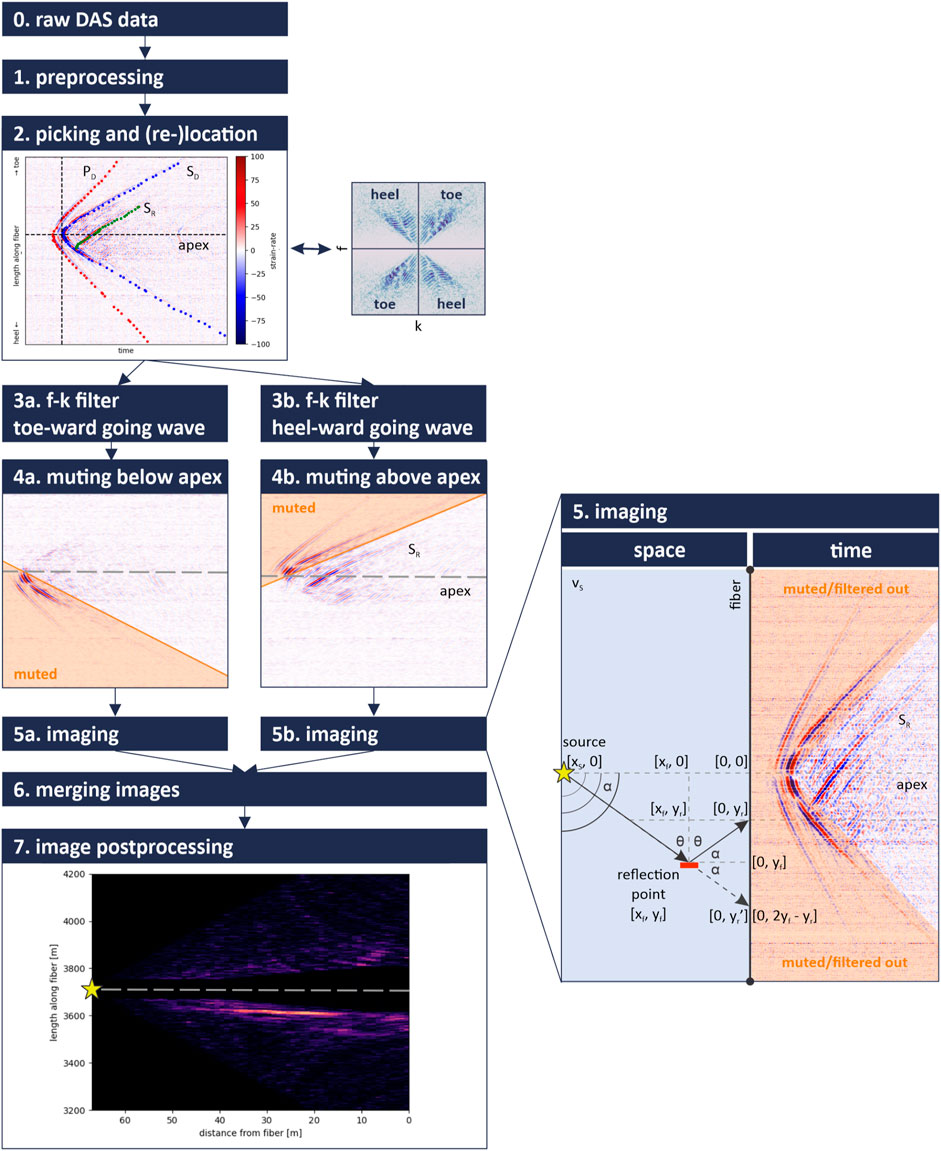
FIGURE 2. Proposed 7-step workflow of reflector imaging using reflected S-waves recorded by DAS with an illustration of raytracing-based reflector imaging methodology.

where $c o s (α) = (x_{s} - x_{f}) / \sqrt{{(x_{s} - x_{f})}^{2} + y_{f}^{2}}$ . The channel y_r along the fiber where the ray of reflected S-wave arrives is:

y_{r} = y_{f} - \frac{x_{f} y_{f}}{x_{s} - x_{f}} . (2)

The DAS data amplitude from the channel y_r at the time tt is then assigned to the tested reflection point in space. After going through all the potential reflection points along the fiber and between the fiber and the event location (we use a regular grid with 1 m spacing), the imaging is done. The imaging result projects the signal amplitude into the imaging spatial grids without amplitude correction. The directional sensitivity of the fiber and the source radiation pattern determines the image amplitude.

The final two steps are (6) merging the two images of toe-ward going and heel-ward going reflected waves to form a complete image and (7) image post-processing. Here, we calculate signal envelopes and apply a low-pass filter to the merged image to further enhance the visibility of the reflector(s). An example of the resulting image is shown at the bottom of the workflow, where the dark color means no reflection or data coverage, and coherent near-horizontal bright spots represent positions of near-vertical reflectors approximately perpendicular to the fiber.

3 Results

3.1 Imaged Reflectors

We demonstrate the processing results for two example microseismic events (Events A and B displayed in Figure 1) using the above-described methodology. Figure 3 shows input DAS microseismic waveforms and the resulting images of reflectors in space in two columns on the left. Each image is a 2D plane connecting the event location and the part of the fiber from which we have DAS data.

FIGURE 3

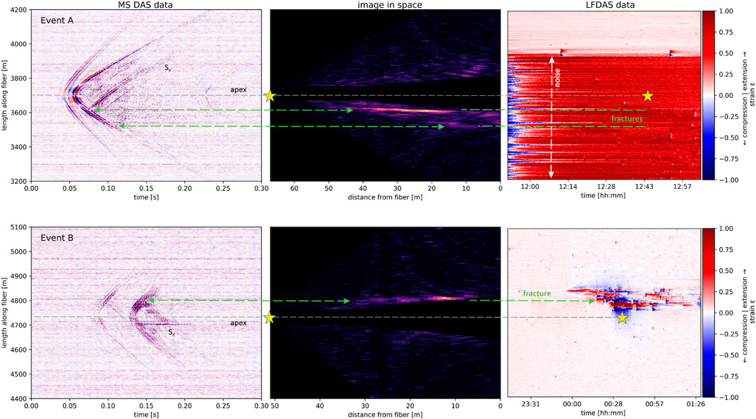
FIGURE 3. Input DAS data, reflector images, and LFDAS data for two example events. The green dashed-line arrows highlight the positions of reflectors in the images. The yellow stars represent the location and origin time (only in the LFDAS data) of microseismic events.

The bright spots elongated in the direction approximately perpendicular to the fiber indicate the imaged reflectors. The length of imaged reflectors is proportional to the length of the reflected wave visible in the DAS data. The imaged reflectors usually do not intersect with the fiber (at the distance 0) because of the mute window around the direct arrivals (including a few wavelengths of high-amplitude S-wave coda). The muting must be done to avoid distortion of the final image around the apex. However, we realize that we also mute part of the reflected S-wave signal mixed with S-wave coda and thus lose information about the reflector in the vicinity of the fiber. The imaged reflectors fade out with distance from the fiber similar to the high-amplitude signal of the reflected wave in the DAS data. It does not mean that the actual reflectors cannot be longer, we image only the sections between hypocenter and fiber illuminated by the S-wave of the individual microseismic event. The signal-to-noise ratio (SNR) of reflected waves depends on event magnitude, distance of the event from the fiber (attenuation and geometrical spreading), and noise in the data.

The black color at a far distance from the fiber means no data coverage, i.e., there are no points reflecting energy back to the part of the fiber we have data from. Whereas the black spaces in a narrow zone around the apex line results from muting the direct S-wave in the input data (steps (4a) and (4b) of the workflow). All the other spaces with dark colors represent media without reflectors.

The image of Event A shows one very clear horizontal bright spot, representing a reflector within 50 m from the fiber. In the DAS data, the position of the imaged reflector along the fiber corresponds to the channel where both direct S- and reflected S-waves intersect (highlighted by green dashed-line arrow in the Figure 3). There is another reflector in the image which is weaker and shorter (visible within 20 m from the fiber) than the main reflector but still has coherent brightness in the approximately perpendicular direction from the fiber. The matching reflected S-wave in the DAS data is of proportionally low SNR and its amplitude quickly attenuates away from the fiber. The remaining randomly located bright spots are too small and probably result from coherent noise in the input data. Meanwhile, Event B has one approximately 30 m long reflector visible in its image.

3.2 Comparison With LFDAS and Interpretation

Up to this point, we have referred to bright spots in images as reflectors because we had no clear indication of whether they can be interpreted as newly created fractures due to hydraulic fracturing or pre-existing vertical faults in the area. To inspect whether we have imaged one or the other, we compared the images with LFDAS data. The LFDAS data are the same recorded raw DAS data as the analyzed DAS microseismic data but in a very low-frequency band ( $<$ 0.1 Hz). Figure 3 shows DAS microseismic data in the left column, images for both microseismic events in the middle, and LFDAS data from the corresponding stage in the right column. The yellow stars placed in the LFDAS data are at the events’ origin time and location along the fiber. Note that the DAS microseismic data of each event and consequently the image of reflector(s) is a snapshot of the medium around the event location at the time when event happened, whereas the LFDAS data show the evolution of measured strain during the entire stage.

The LFDAS data around the origin time and location of Event B show a very clear signal characteristic of frac-hits. The first fracture started to open (zone of compression in blue around the extensive opening zone in red) shortly before 12 a.m. Later on, other fractures hit the fiber approximately 80 m away from the first frac-hit and started to open. A few minutes later, the changes in the reservoir induced Event B, recorded by the DAS array. The comparison with LFDAS provides undeniable evidence that the observed S-wave is back-scattered from the newly created fracture to the monitoring fiber–position of the fracture in our image aligns with the position of frac-hit in the LFDAS data (see the green dashed-line arrow). The explanation of why we identified only one fracture in the image while the LFDAS shows three existing fractures at the event origin time is unclear. It is less likely to be a resolution issue as the thickness of the imaged fracture is smaller than the entire fractured zone. The first open fracture (at the top in the LFDAS) is most likely not imaged due to its narrower width or because the fracture was already closed and did not create enough seismic impedance. The third fracture (at the bottom in the LFDAS) lies in the muted zone of our image (too close to the apex of the microseismic event).

The LFDAS data for the stage of hydraulic fracturing when Event A occurred is of low quality, not allowing detection of frac-hits. The source of abnormally high low-frequency noise was an injection operation taking place in the monitoring well. This caused a large temporal change in temperature conditions in a short time before the LFDAS data were acquired. Note that the low-frequency noise does not affect the DAS microseismic data while we look at much higher frequencies where the sensitivity to temperature is negligible. As the image of Event B has been proven to be showing induced fracture(s), we may expect that the similarly looking reflectors in the image of Event A are also fractures. However, we cannot prove it by comparison with frac-hit due to the noisy LFDAS.

4 Discussion

4.1 Methodology

Our methodology relies on recorded signals reflected from the fractures. We have used reflected S-waves; but analogically, reflected P-waves might be used. Visibility of reflected waves in data depends on sensitivity of the DAS monitoring system, magnitude of microseismic event, impedance contrast related to fracture geometry, width, and volume of fluids in the fracture, and relative geometry between the source, fiber, and fracture. If the fracture width is narrow and the impedance contrast in the medium is not strong enough to reflect enough energy to be detected above background noise level, we cannot see it in the image, of course. If the microseismic event is located too close to the induced fracture (relative to the distance of the event from the fiber), most of the energy is reflected to far offset channels (far from the apex line in the DAS data), and the signal of the reflected wave arrives shortly after the direct body wave and has almost the same moveout. Therefore, in our workflow, the reflected wave may be filtered out or muted together with the body wave signal, and information about fracture is lost. Remaining energy reflected from the fracture appears close to the apex where it is usually mixing with high SNR body-wave coda which we also mute. This means that fracture imaging using reflected waves is hardly possible when the event-fracture-fiber geometry does not lead to a reflected signal clearly distinguishable from the signal of direct body waves.

Our fracture imaging methodology is based on several assumptions. The raytracing is done only for reflections from vertical fractures oriented approximately perpendicular to the fiber in a homogeneous isotropic velocity model. These assumptions appear to be valid only if the fractures are near vertical. Perpendicularity of fractures to a well is expected when lateral parts of both treatment and monitoring wells are drilled in parallel and perpendicularly to the maximum horizontal stress direction in the area. In our case, the observed reflected S-waves with asymmetrical moveout parallel to the moveout of direct S-wave can be explained only with a near-vertical fracture, near-perpendicular to the fiber. The fact that microseismic events and monitor well are in the same horizontal formation allows us to assume a single velocity structure. We were able to fit both P- and S-wave moveouts with the homogeneous velocity model, i.e., without the need to use more complicated models. Similar conditions might be found in many other fields but, in general, to be able to image fractures with arbitrary orientation in a complex velocity model, we would need to use more sophisticated raytracing or advanced imaging methods such as Kirchhoff migration or reverse time migration (e.g., Li et al., 2020). However, that would require more accurate event locations and stacking of many microseismic events (sources) to get a reasonable image.

One of our first steps in the workflow is manual picking and event (re-)location as we wanted to improve the initial event locations obtained from the surface microseismic catalogue. Without the known initial location, we would still locate the event but have only very accurate information about the event position along the fiber and the relatively accurate distance from the fiber when located from one fiber only. The event location would have uncertainty of 360^o around the axis of the horizontal well because of the axial sensitivity of DAS. Therefore, we would not know the correct orientation of the imaged fractures. Note that the image is always in the plane connecting the event location and the fiber. We have not thoroughly tested the effect of uncertainty in event distance from the fiber on the imaged fracture as the uncertainty in horizontal location for our selected events is in the order of a few meters and the changes in images were negligible. Of course, P- and S-wave arrivals needed for location do not have to be picked manually if an efficient auto-picking algorithm is employed.

4.2 Application

The most obvious application of fracture imaging is the processing of continuous cross-well DAS microseismic data acquired during hydraulic fracturing to map created fractures around stimulated wells. Such detailed map can have a big impact on the precision of DFN and its reliability. With fracture imaging, we may potentially map the dynamic evolution of the fracture if several microseismic events are induced and detected during the same stage around the fracture reflecting energy. The microseismic events provide snapshots of the surrounding reservoir at their origin times. If we are able to image fractures, it means that the fracture is already open and wide enough to reflect energy emitted by nearby microseismic events. With several microseismic events following each other in time, we may see fracture growth, i.e., dynamic changes of the reflected wave visible in DAS data, and thus the lateral extent of the imaged fractures. When the fracture starts closing, seismic impedance decreases, and the fracture disappears from the image. Fracture closing was shown in LFDAS data by Jin and Roy (2017) as well as in time-lapse DAS VSP. Compared to the 4D inter-stage DAS VSP (Binder et al., 2020; Titov et al., 2021), our fracture imaging provides a better resolution due to higher frequency content (microseismic event as a source is closer to the fiber than the surface source used for VSP) and can image fractures in 3D if the event location is known.

While the fracture visibility in the images depends on impedance contrast in the medium, fracture images might be used for estimation of fracture width or volume of fluids in the fracture. However, such impedance dependency on the mentioned parameters is not known at this time. We plan to study the effect of uncertain microseismic event location on the image, perform AVO analyses on the reflector for more quantitative analyses of the imaging results, and estimate fracture properties using reflected S-wave.

Due to the above-described assumptions and limitations of the methodology, we do not claim that we are imaging all possibly existing fractures. The presented fracture imaging can be understood as a very powerful method providing important but only additional information about the whole fracture system induced by hydraulic fracturing, which may be integrated with available results of other methods mapping fractures. For example, location of microseismic events, fault planes of inverted source mechanisms (size of planes is proportional to magnitudes), or frac-hits also provide information about fracture propagation and geometry. In this study, we used LFDAS data showing frac-hits. Unfortunately, as shown in the example in Figure 3, LFDAS can be contaminated by noise due to temperature effects induced by injection operations in the monitor well. In such cases, fracture imaging using DAS microseismic data may provide complementary information to results from LFDAS. Furthermore, the LFDAS can detect frac-hits or strain changes only in the close vicinity of the monitoring fiber. Our fracture imaging is also able to map these frac-hits and, moreover, it has the capability to map fractures which does not intersect monitoring fiber well, as the imaging space is located between the event and the monitoring fiber. From such images, we can estimate the fracture geometry of fractures with half-length shorter than well spacing. Of course, the disadvantage is that fracture imaging is dependent on induced microseismic events, whereas LFDAS is not.

5 Conclusion

We have shown examples of microseismic events recorded by DAS fiber in a horizontal well during hydraulic fracturing of an unconventional reservoir. Besides direct P- and S-waves, the events have visible signals of S-waves reflected at hydraulic fractures. We developed a new processing workflow to image the fracture using the reflected waves and demonstrated the conversion of DAS-based microseismic data in time to fracture image in space. The resulting images were compared to frac-hit signals in corresponding LFDAS data, supporting that the imaged reflectors are newly created hydraulic fractures. The fracture imaging can be further developed with a potential to be used for a real-time 3-D hydraulic fracture development mapping when DAS monitoring is employed and induced microseismic events are detected in abundance.

Data Availability Statement

The DAS microseismic data of events A and B used as examples for fracture imaging in this study are available from the corresponding author upon request.

Author Contributions

FS and GJ co-developed the presented idea. FS developed the workflow, performed data processing, made all the figures, and wrote the first draft of the manuscript. GJ supervised the progress of the work and edited the manuscript. JS contributed to discussions and edited the manuscript.

Funding

This work was conducted with the support of the Reservoir Characterization Project (Phase XVIII.) at the Colorado School of Mines.

Conflict of Interest

The authors declare that the research was conducted in the absence of any commercial or financial relationships that could be construed as a potential conflict of interest.

Publisher’s Note

All claims expressed in this article are solely those of the authors and do not necessarily represent those of their affiliated organizations, or those of the publisher, the editors, and the reviewers. Any product that may be evaluated in this article, or claim that may be made by its manufacturer, is not guaranteed or endorsed by the publisher.

Acknowledgments

The authors are thankful to Civitas Inc. for support, providing the data and permission to publish the results. The authors thank Alicia Downard for helping with orientation in the data and providing seismic coherence maps (used in Figure 1), and Xiaoyu (Rosie) Zhu for helping with the LFDAS data.

References

Baird, A., Stork, A., Horne, S., Naldrett, G., Kendall, M., Wookey, J., et al. (2019). “Modelling of Fibre-Optic DAS Response to Microseismic Arrivals in Anisotropic Media,” in 81st EAGE Conference and Exhibition 2019 (London, UK: European Association of Geoscientists & Engineers), 1–6. doi:10.3997/2214-4609.201901244