Investigation of the Global Seismic Noise Properties in Connection to Strong Earthquakes

The global seismic noise, recorded on a network of 229 broadband seismic stations located around the globe for 25 years, from the beginning of 1997 to the end of 2021, has been investigated. To study the noise properties a set of statistics estimated daily have been used: the multifractal singularity spectrum support width, the minimum entropy of the squared wavelet coefficients, and the wavelet-based Donoho-Johnstone (DJ) index. It is shown that the time points of local extrema of the average values of the analyzed noise properties (minima for singularity spectrum support width and DJ-index and maxima for entropy) tend to occur before strong earthquakes. The time interval from the middle of 2002 to the middle of 2003 is determined, when the trend of decreasing the average coherence of the noise properties in the auxiliary network of 50 reference points changed to an increase. Along with an increase in the average coherence, there is an increase in the radius of the spatial maximum coherences of noise properties. Both of these trends continue until the end of 2021, which is interpreted as a general sign of an increase in the degree of criticality of the state of the planet and, as a result, an increase in global seismic danger. After two mega-earthquakes close in time: 27 February 2010, M=8.8 in Chile and 11 March 2011, M=9.1 in Japan, there was an increase in the spatial scales of the strong coherence of noise parameters, which is a sign of an increase in the critical state. The response of seismic noise properties to variations in the length of the day (LOD) has been studied. An estimate of the correlation function between the mean values of the response to LOD and the logarithm of the released seismic energy in a time window of 1 year indicates a delay in energy release with respect to the maxima of the response of noise properties to LOD with a delay time of about 500 days. In connection with this result, an additional intrigue is the extreme increase in the average value of the response to LOD in 2021.

Introduction

In (Kobayashi and Nishida, 1998; Tanimoto, 2001; Rhie and Romanowicz, 2004; Tanimoto, 2005; Aster et al., 2008; Kedar et al., 2008; Nishida et al., 2008; Nishida et al., 2009; Ardhuin et al., 2011) it was shown that the energy source of low-frequency seismic noise is the processes occurring in the ocean and atmosphere. Since the earth’s crust is the propagation medium for seismic waves, changes in the lithosphere are reflected in the statistical properties of the noise. Analysis of changes in these properties makes it possible to evaluate the effects associated with the seismic process occurring in different regions of the Earth and at the global level. Changes of seismic noise spectral parameters in different frequency bands in India during the nationwide COVID-19 lockdown were estimated in (Pandey et al., 2020). Seismic noise in the frequency range 0.5–18 Hz continuously recorded by seismic network in the Central Italy before L’Aquila earthquake, 2009, was investigated in details in (Shi et al., 2020).

The article continues the studies carried out in (Lyubushin, 2014; Lyubushin, 2015; Lyubushin, 2018; Lyubushin, 2020a; Lyubushin, 2020c; Lyubushin, 2021c) to investigate the correlation and coherence properties of low-frequency seismic noise on a global scale covering the entire planet. Since 1997, the total number of broadband seismic stations from various networks has become quite large (229 stations), and their location provides satisfactory coverage of the earth’s surface. This makes it possible to estimate the spatial and temporal correlations of various properties of seismic noise and compare the identified features with the seismic process. The multifractal singularity spectrum support width, the minimum entropy of squared orthogonal wavelet coefficients, and the Donoho-Johnstone index, equal to the ratio of the number of “large” wavelet coefficients to their total number, were considered as main properties of seismic noise. These noise statistics were evaluated for each station in successive time intervals of 1 day. An auxiliary network of 50 reference points is introduced, distributed over the Earth’s surface, for each of which daily time series of median values of seismic noise properties from 5 nearest operational stations were calculated. In a sliding time window with a length of 365 days, the mean moduli of the pairwise correlation coefficients of the daily noise properties between the values at all reference points were estimated. It turned out that the behavior of average correlations for all properties has a common qualitative feature: before 2003, a decrease is observed, but after 2003, a rapid increase in correlation begins. In (Lyubushin, 2020a; Lyubushin, 2020c), it was hypothesized that the break in the average correlation trends in 2003 is due to a high-frequency anomaly in the Earth’s rotation regime, which can also be a trigger for an increase in the intensity of the strongest seismic events after the Sumatran mega-earthquake on 26 December 2004. The kink in the trend of correlations in 2003 is accompanied by a kink in the trends of the values of the seismic noise properties being analyzed: after 2003, the average widths of the carrier of the singularity spectrum support width and DJ-index decrease, and the average values of the noise entropy increase. This behavior of seismic noise properties (simplification of the statistical structure) considered as an indicator of an increase in seismic hazard (Lyubushin, 2018; Lyubushin, 2021a; Lyubushin, 2021b). Thus, the simplification of the statistical structure of seismic noise and the increase in their spatial correlations occur synchronously, and this behavior can be interpreted as an increase in the global seismic hazard.

The methodological basis of the used approach to data analysis is the general property of synchronization of the behavior of the constituent parts of complex systems as they approach critical states (Gilmore, 1981; Nicolis and Prigogine 1989). The goal of all methods used is to search for synchronization effects by estimating the coherence of seismic noise in different regions of the planet.

Seismic Noise Statistics

Let $x\left(t\right)$ be a time series of a random signal and $t=1,\mathrm{...},N$ let be an integer index numbering successive data points (discrete time). The normalized entropy of a finite sample is given by the following formula:

$En=-{\displaystyle \sum _{k=1}^N{p}_k\cdot \log \left(p_k\right)/\log \left(N\right)},p_k=c_k^2/{\displaystyle \sum _{j=1}^N{c}_j^2},0\le En\le 1(1)$

where $c_k$ are orthogonal wavelet coefficients. Let us choose the optimal orthogonal wavelet for the sample under consideration from the entropy minimum condition (1) on a finite set of Daubechies wavelet bases (Mallat, 1999) with the number of vanishing moments from 1 to 10. After the wavelet basis is determined for a given signal from the entropy minimum condition, we can determine the set of wavelet coefficients that are the smallest in absolute value. We assume that the noise is concentrated mainly in variations at the first highest frequency level of detail.

Seismic noise entropy (1) was used in (Lyubushin, 2014; Lyubushin, 2015; Lyubushin, 2017; Lyubushin, 2018; Lyubushin, 2020a; Lyubushin, 2020b; Lyubushin, 2020c; Lyubushin, 2021a; Lyubushin, 2021b; Lyubushin, 2021c) to analyze seismic noise for different regions of the Earth and at the global level as a standalone tool. By its design, entropy (1) is also multiscale, like the entropy proposed in (Costa et al., 2003; Costa et al., 2005) for studying the properties of random signals. In (Koutalonis and Vallianatos, 2017; Vallianatos et al., 2019) the non-extensive entropy of Tsallis was used to analyze seismic noise. The natural time approach to the analysis of random data uses a related definition of entropy in (Varotsos et al., 2003a; Varotsos et al., 2003b; Varotsos et al., 2004; Varotsos et al., 2011).

The noise standard deviation is estimated as the standard deviation of the wavelet coefficients at the first detail level of wavelet decomposition. This estimate must be stable, i.e., insensitive to outliers in the values of the wavelet coefficients at the first level. To do this, we can use a robust median estimate of the standard deviation for a normal random variable:

$\sigma =med\left\{\left|c_k^{\left(1\right)}\right|,k=1,\mathrm{...},N/2\right\}/0.6745,(2)$

where $c_k^{\left(1\right)}$ are wavelet coefficients at the first level of detail; $N/2$ is the number of such coefficients. The estimate of the standard deviation $\sigma$ from formula (2) determines the value $\sigma \sqrt{2\cdot \ln N}$ as a “natural” threshold for extracting noise wavelet coefficients. This quantity is known in wavelet analysis as the Donoho–Johnstone threshold (Donoho and Johnstone, 1995; Mallat, 1999). As a result, we can define the dimensionless signal characteristic $\gamma$, $0<\gamma <1$, as the ratio of the number of the most informative wavelet coefficients for which the inequality $\left|c_k\right|>\sigma \sqrt{2\cdot \ln N}$ is satisfied to the total number $N$ of all wavelet coefficients. Formally, the larger the index $\gamma$, the less noisy the signal is.

Qualitatively, the multifractal singularity spectrum $F\left(\alpha \right)$ for a random signal $x\left(t\right)$ can be defined as the fractal dimensionality of the set of time points $t$, for which the Holder-Lipschitz exponent is $\alpha$, which means $|x\left(t+\delta \right)-x\left(t\right)|\sim |\delta {|}^{\alpha },\delta \to 0$. The quantitative calculation of the singularity spectrum requires the introduction of some auxiliary quantities (Feder, 1988). Let’s define the measure of variability ${\mu }_X\left(t,\delta \right)$ of a random signal $x\left(t\right)$ on a time interval $\left[t,t+\delta \right]$ as its range

${\mu }_x\left(t,\delta \right)=\underset{t\le u\le t+\delta }{\max }x\left(u\right)-\underset{t\le u\le t+\delta }{\min }x\left(u\right)(3)$

Signal is a scale-invariant (Feder, 1988), if $M\left(\delta ,q\right)\text{∼}{\delta }^{\rho \left(q\right)}$, when $\delta \to 0$ i.e. the next limit exists:

$\rho \left(q\right)=\underset{\delta \to 0}{\lim }\left(\ln M\left(\delta ,q\right)/\ln \delta \right)(4)$

The signal is mono-fractal if $\rho \left(q\right)=Hq$, $H=const,0<H<1$. If $\rho \left(q\right)$ is a nonlinear concave function of $q$ the signal is multi-fractal. The value of $\rho \left(q\right)$ for a finite sample could be calculated by detrended fluctuation analysis (DFA) (Kantelhardt et al., 2002). The time series is split into adjacent intervals of the length $s$:

$I_k^{\left(s\right)}=\left\{t:1+\left(k-1\right)s\le t\le ks,k=1,\mathrm{...},\left[N/s\right]\right\}(5)$

Let’s consider a part of $x\left(t\right)$ corresponding to the interval $I_k^{\left(s\right)}$:

$y_k^{\left(s\right)}\left(t\right)=x\left(\left(k-1\right)s+t\right),t=1,\mathrm{...},s(6)$

Let $p_k^{\left(s,m\right)}\left(t\right)$ be a polynomial of the order $m$ which is fitted to $y_k^{\left(s\right)}\left(t\right)$ and let’s consider deflections:

$\text{Δ}{y}_k^{\left(s,m\right)}\left(t\right)=y_k^{\left(s\right)}\left(t\right)-p_k^{\left(s,m\right)}\left(t\right),t=1,\mathrm{...},s(7)$

and the sum:

$Z^{\left(m\right)}\left(q,s\right)={\left({\displaystyle \sum _{k=1}^{\left[N/s\right]}{\left(\underset{1\le t\le s}{\max }\text{Δ}{y}_k^{\left(s,m\right)}\left(t\right)-\underset{1\le t\le s}{\min }\text{Δ}{y}_k^{\left(s,m\right)}\left(t\right)\right)}^q}/\left[N/s\right]\right)}^{1/q}(8)$

The value (8) could be regarded as an estimate of ${\left(M\left({\delta }_s,q\right)\right)}^{1/q}$. Let’s consider a function $h\left(q\right)$ as a linear regression coefficient between $\ln \left(Z^{\left(m\right)}\left(q,s\right)\right)$ and $\ln \left(s\right)$: $Z^{\left(m\right)}\left(q,s\right)\sim s^{h\left(q\right)}$ within range of scales $s_{\min }\le s\le s_{\max }$. Minimum value of the scale $s$ in the formulae (5-8) was chosen 20, maximum value—$s_{\max }=N/5$. For mono-fractal signal $h\left(q\right)=H=const$, in general case $\rho \left(q\right)=qh\left(q\right)$. The Gibbs sum is defined as (Feder, 1988):

$W\left(q,s\right)={\displaystyle \sum _{k=1}^{\left[N/s\right]}{\left(\underset{1\le t\le s}{\max }\text{Δ}{y}_k^{\left(s,m\right)}\left(t\right)-\underset{1\le t\le s}{\min }\text{Δ}{y}_k^{\left(s,m\right)}\left(t\right)\right)}^q}(9)$

The mass index $\tau \left(q\right)$ is defined from the condition $W\left(q,s\right)\sim s^{\tau \left(q\right)}$. Formula $\tau \left(q\right)=\rho \left(q\right)-1=qh\left(q\right)-1$ is the consequence of (8). The values of $q$ in the formula (8) are taken from interval $\left[-Q,+Q\right]$ where $Q$ is some a priory large number (the value $Q=10$ was used). The function $F\left(\alpha \right)=\underset{q\in \left[-Q,+Q\right]}{\min }\left(\alpha q-\tau \left(q\right)\right)$ is calculated for $\alpha \in \left[A_{\min },A_{\max }\right]$ where $A_{\min }=\underset{q\in \left[-Q,+Q\right]}{\min }d\tau \left(q\right)/dq$ and $A_{\max }=\underset{q\in \left[-Q,+Q\right]}{\max }d\tau \left(q\right)/dq$. The derivative $d\tau \left(q\right)/dq$ is calculated numerically. Its accuracy is nonessential because this derivative was used for rough estimate of a priory interval of $\alpha$ values. Values of ${\alpha }_{\min }$ and ${\alpha }_{\max }$ are defined as minimum and maximum $\alpha$, for which $F\left(\alpha \right)\ge 0$. Thus, multi-fractal spectrum $F\left(\alpha \right)$ is defined according to formula:

$F\left(\alpha \right)=\max \left\{\underset{q\in \left[-Q,+Q\right]}{\min }\left(\alpha q-\tau \left(q\right)\right),0\right\}(10)$

Let’s consider estimates of singularity spectrum $F\left(\alpha \right)$ within moving time window. In this case its evolution could provide important information about the structure of chaotic pulsations of time series. In particular the singularity spectrum support width $\text{Δ}\alpha ={\alpha }_{\max }-{\alpha }_{\min }$ is regarded as a measure of complexity of stochastic behavior.

Multifractal analysis is an instruments which is used in geophysical studies rather actively (Ramirez-Rojas et al., 2004; Currenti et al., 2005; Ida et al., 2005; Telesca et al., 2005; Chandrasekhar et al., 2016). The multifractality of seismic noise was used for earthquake prediction and seismic hazard assessment in (Lyubushin, 2010; Lyubushin, 2012; Lyubushin, 2013; Lyubushin, 2018; Lyubushin, 2021a). The singularity spectrum support width is used to study the behavior of various nonlinear systems. A decrease in the parameter $\text{Δ}\alpha$ is a well-known effect that anticipates changes in the properties of biological and medical systems (Ivanov et al., 1999; Pavlov and Anishchenko, 2007). In (Pavlov and Anishchenko, 2007) it is shown that the “loss of multifractality” is also universal in physical systems. The natural time approach has its own tools using multifractals and multi-scale entropy for seismicity analysis (Varotsos et al., 2014; Sarlis et al., 2015).

First Principal Component

The values of the parameters $\left(\gamma ,\Delta \alpha ,En\right)$ introduced above are calculated in successive time windows of a certain length, resulting in a 3-dimensional time series, the properties of which are further studied jointly. The used properties of seismic noise reflect the change in its structure, in particular, we are interested in the phenomenon of noise structure simplification as a sign that precedes strong earthquakes. Attempts to determine the “best” property of noise led to the idea of using the principal component approach (Jolliffe, 1986) to aggregate time series $\left(\gamma ,\Delta \alpha ,En\right)$ into one scalar time series. Since the purpose of the analysis is to study the variability of noise properties both in time and space, the principal component method was applied in a sliding time window. The modification of the principal component method was proposed in (Lyubushin, 2018).

Let’s consider a multiple time series $P\left(t\right)={\left(P_1\left(t\right),\mathrm{...},P_m\left(t\right)\right)}^T$, $t=\mathrm{0,1},\mathrm{...}$ of the dimensionality $m$ (in our case $m=3$). It is necessary to estimate its first principal component in the moving time window of the length $L$ samples. For this purpose let’s consider samples with time indices $t$ under the condition $s-L+1\le t\le s$ where $s$ is the right-most end of moving time window. Correlation matrix $\text{Φ}\left(s\right)$ of the size $m\times m$ is calculated by the formula:

$\mathrm{\Phi }\left(s\right)=\left({\phi }_{ab}^{\left(s\right)}\right),{\phi }_{ab}^{\left(s\right)}={\displaystyle \sum _{t=s-L+1}^s{q}_a^{\left(s\right)}\left(t\right)q_b^{\left(s\right)}\left(t\right)/L,a,b=1,\mathrm{...},m}(11)$

$\begin{array}{l}{q}_a^{\left(s\right)}\left(t\right)=\left(P_a\left(t\right)-{\overline{P}}_a^{\left(s\right)}\right)/{\sigma }_a^{\left(s\right)},{\overline{P}}_a^{\left(s\right)}={\displaystyle \sum _{t=s-L+1}^s{P}_a\left(t\right)/L,}{\left({\sigma }_a^{\left(s\right)}\right)}^2=\\ ={\displaystyle \sum _{t=s-L+1}^s{\left(P_a\left(t\right)-{\overline{P}}_a^{\left(s\right)}\right)}^2/\left(L-1\right)},a=1,\mathrm{...},m\end{array}(12)$

Let ${\theta }^{\left(s\right)}={\left({\theta }_1^{\left(s\right)},\mathrm{...},{\theta }_m^{\left(s\right)}\right)}^T$ be eigenvector of the matrix $\Phi \left(s\right)$ corresponding to its maximum eigenvalues. Let’s define 1^st principal component within current time window:

${\psi }^{\left(s\right)}\left(t\right)={\displaystyle \sum _{\alpha =1}^m{\theta }_a^{\left(s\right)}\cdot q_a^{\left(s\right)}\left(t\right)}(13)$

and define scalar time series $\psi \left(t\right)$ of the adaptive first principal component in the moving time window by the formula:

$\psi \left(t\right)=\{\begin{array}{c}{\psi }^{\left(L-1\right)}\left(t\right),0\le t\le \left(L-1\right)\\ {\psi }^{\left(t\right)}\left(t\right),t\ge L\end{array}(14)$

Formulae (11-14) are applied independently within each time window. According to these formulae within first time window time series $\psi \left(t\right)$ consists of $L$ values corresponding to (13, 14). In all subsequent windows $\psi \left(t\right)$ corresponds the only sample in the right-most time index. Thus, outside the first time window $\psi \left(t\right)$ is dependent on the past values of $P\left(t\right)$.

Hereinafter, a window with a length of 365 days will be used. The choice of this length is quite natural because of presence of annual periodicity in almost all background processes in Earth’s crust. Next, the first principal component is calculated, that is, the projection of all components of the 3-dimensional time series after normalizing them to unit variance onto this eigenvector. In the first time window, the principal component is equal to the projection values for all samples within this window, and for subsequent windows, only one value is taken, corresponding to the rightmost time sample of the window. Thus, outside the first time window, the principal component depends only on past values with a memory depth equal to the length of the window.

It should be noticed that values of seismic noise parameters $\left(\gamma ,\text{Δ}\alpha ,En\right)$ and their first principal component are dimensionless.

Global Seismic Noise Data

The data used are the vertical components of continuous seismic noise records at 1 s sampling intervals, which were downloaded from the Incorporated Research Institutions for Seismology (IRIS) website at http://www.iris.edu/forms/webrequest/from 229 broadband seismic stations of 3 networks: http://www.iris.edu/mda/_GSN, http://www.iris.edu/mda/G, http://www.iris.edu/mda/GE.

Seismic noise records with a sampling rate of 1 Hz (LHZ records) were considered for 25 years of registration (from 1 January, 1997 to 31 December, 2021). These data were converted to 1-min time series by calculating averages for successive 60-s time intervals. Estimates of spectral power densities after coming to 1-min time step were presented in (Lyubushin, 2020c). The analysis is restricted by vertical component only because behaviors of multi-fractal and entropy properties of the noise which are used in the paper are rather typical for all components of seismic noise in the investigated range of periods exceeding 2 min.

Consider an auxiliary network of 50 reference points, which are determined using a hierarchical cluster analysis of the positions of 229 seismic stations using the “far neighbor” method. This method of cluster analysis makes it possible to form compact clusters (Duda et al., 2000). The location of 229 seismic stations and 50 reference points is shown in Figure 1A.

FIGURE 1

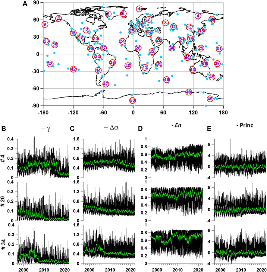
FIGURE 1. (A)—positions of 229 seismic stations (blue circles) and 50 reference points (numbered red circles); (B–D)—plots of daily values of 3 properties of seismic noise $\gamma$, $\text{Δ}\alpha$ and $En$, corresponding to reference points with numbers 4, 20 and 34; (E)—plots of the first principal component of noise properties calculated in a sliding time window of 365 days length for the specified reference points. The green lines represent moving average graphs in a 57-day window. Values of $\gamma$, $\text{Δ}\alpha$, $En$ and first principal component are dimensionless.

Figures 1B–D show examples of plots of daily property values of $\left(\gamma ,\text{Δ}\alpha ,En\right)$ for three reference points numbered 4, 20 and 34, calculated as median values from the 5 nearest stations that are operational on each day. The values of these properties at all other reference points are calculated in the same way. Before calculating the properties from the daily waveforms of seismic noise with a length of 1440 min, the trend is removed by a polynomial of the 8th order. This choice of detrending polynomial order is discussed in details in (Lyubushin, 2021a). The 8th order of trend polynomial provides removing of complicated low-frequency daily waveforms which occur due to the influence of tides and diurnal temperature effects. Figure 1E shows the graphs of the first principal components of properties $\left(\gamma ,\Delta \alpha ,En\right)$ in a moving time window of 365 days for the same reference points with numbers 4, 20, and 34. The green lines show the graphs of moving averages in a window of 57 days. The window length of 57 days was chosen experimentally as a value that, on the one hand, smooths high-frequency pulsations of daily median seismic noise properties, and on the other hand, allows one to see the annual frequency of changes in these properties. The number 57 equals to double length of Moon month (28 days) plus 1. An additional unit is needed to make the window length odd.

Analysis of the Relationship Between Extremum Points of Noise Properties and Strong Earthquakes

In (Lyubushin, 2010; Lyubushin, 2012; Lyubushin, 2013; Lyubushin, 2014; Lyubushin, 2018; Lyubushin, 2021a; Lyubushin, 2021b), the hypothesis was used that an increase in seismic hazard is preceded by a decrease in the singularity spectrum support width $\text{Δ}\alpha$ and the DJ index $\gamma$, as well as an increase in entropy $En$. In the analysis of global seismicity, one can independently test this idea by analyzing the relationship between two point processes: a sequence of strong earthquakes with magnitude $M\ge 7$ and time points of local extrema of the average values of noise properties: minima for $\text{Δ}\alpha$, $\gamma$ and maxima for $En$. During the period of time 1997–2021 there were 377 earthquakes $M\ge 7$. Therefore, for comparison, we will also select 377 time points of the most “expressive” local extrema, which have the largest amplitude of deviation from the local average. We calculate the local average at each moment of time by smoothing the mean values of the noise properties by a Gaussian kernel (Hardle, 1990) with an averaging radius of 2 days. This is a minimum length of vicinity which provides efficient removing of local mean value and extracting extremum spikes. To test the hypothesis, it is necessary to analyze the relationship between the time moments of earthquakes and the positions of local minima and local maxima. It is expected that “on average” local minima $\Delta \alpha$, $\gamma$ and local maxima $En$ will precede earthquakes, while for local maxima and local minima the opposite effect should be observed. In addition, the variability of the links between the analyzed point processes in time is of interest, that is, it is desirable to carry out the analysis in a sliding time window.

For the analysis of mutual relationships between point processes, the method of influence matrices (Lyubushin and Pisarenko, 1994), developed to analyze the relationships between several sequences of seismic events from different regions, was used. Further, a simplified version of the model is used for the case of analysis of relationships between two sequences. It can be considered as an analogue of the classical cross-correlation method.

Let $t_j^{\left(\alpha \right)},j=1,\mathrm{...},N_{\alpha };\alpha =\mathrm{1,2}$ represent moments of time of 2 streams of events. Let’s consider their intensities in the form:

${\lambda }^{\left(\alpha \right)}\left(t\right)=b_0^{\left(\alpha \right)}+{\displaystyle \sum _{\beta =1}^2{b}_{\beta }^{\left(\alpha \right)}\cdot g^{\left(\beta \right)}\left(t\right)}(15)$

where $b_0^{\left(\alpha \right)}\ge 0,b_{\beta }^{\left(\alpha \right)}\ge 0$ are parameters, $g^{\left(\beta \right)}\left(t\right)$ is a function of influence of the events $t_j^{\left(\beta \right)}$ from the stream with number $\beta$:

$g^{\left(\beta \right)}\left(t\right)={\displaystyle {\sum }_{t_j^{\left(\beta \right)}<t}\exp \left(-\left(t-t_j^{\left(\beta \right)}\right)/\tau \right)}(16)$

According to formula (15), the weight of the event with the number $j$ becomes non-zero for times $t>t_j^{\left(\beta \right)}$ and decays with the characteristic time $\tau$. The parameter $b_{\beta }^{\left(\alpha \right)}$ determines the degree of influence of the flow $\beta$ on the flow $\alpha$. The parameter $b_{\alpha }^{\left(\alpha \right)}$ determines the degree of influence of the flow on itself (self-excitation), and the parameter $b_0^{\left(\alpha \right)}$ reflects a purely random (Poisson) intensity component. We fix the parameter $\tau$ and consider the problem of determining the parameters $b_0^{\left(\alpha \right)},b_{\beta }^{\left(\alpha \right)}$. The log-likelihood for a non-stationary Poisson process over a time interval $\left[0,T\right]$ is (Cox and Lewis, 1966):

$\ln \left(L_{\alpha }\right)={\displaystyle \sum _{j=1}^{N_{\alpha }}\ln \left({\lambda }^{\left(\alpha \right)}\left(t_j^{\left(\alpha \right)}\right)\right)-{\displaystyle \underset{0}{\overset{T}{\int }}{\lambda }^{\left(\alpha \right)}\left(s\right)ds}},\alpha =\mathrm{1,2}(17)$

It is necessary to find the maximum of functions (16) with respect to the parameters $b_0^{\left(\alpha \right)},b_{\beta }^{\left(\alpha \right)}$. It is easy to get the following expression:

$b_0^{\left(\alpha \right)}\frac{\partial \ln \left(L_{\alpha }\right)}{\partial b_0^{\left(\alpha \right)}}+{\displaystyle \sum _{\beta =1}^2{b}_{\beta }^{\left(\alpha \right)}\frac{\partial \ln \left(L_{\alpha }\right)}{\partial b_{\beta }^{\left(\alpha \right)}}}=N_{\alpha }-{\displaystyle \underset{0}{\overset{T}{\int }}{\lambda }^{\left(\alpha \right)}\left(s\right)ds}(18)$

Since the parameters $b_0^{\left(\alpha \right)},b_{\beta }^{\left(\alpha \right)}$ must be non-negative, then each term on the left side of this formula is equal to zero at the maximum point of function (16) - either due to the necessary extremum conditions (if the parameters are positive), or, if the maximum is reached at the boundary, then the parameters themselves are equal to zero. Therefore, at the maximum point of the likelihood function, the following equality holds:

${\displaystyle \underset{0}{\overset{T}{\int }}{\lambda }^{\left(\alpha \right)}\left(s\right)ds=N_{\alpha }}(19)$

Substitute the expression $g^{\left(\beta \right)}\left(t\right)$ from (15)–(18) and divide by $T$. Then we get another form of formula (18):

$b_0^{\left(\alpha \right)}+{\displaystyle \sum _{\beta =1}^m{b}_{\beta }^{\left(\alpha \right)}\cdot {\overline{g}}^{\left(\beta \right)}={\lambda }_0^{\left(\alpha \right)}\equiv }{N}_{\alpha }/T(20)$

where

${\overline{g}}^{\left(\beta \right)}={\displaystyle {\int }_0^T{g}^{\left(\beta \right)}\left(s\right)ds}/T(21)$

- The average value of the influence function. Substituting $b_0^{\left(\alpha \right)}$ from (19), (16), we obtain the following maximum problem:

${\Phi }^{\left(\alpha \right)}\left(b_1^{\left(\alpha \right)},b_2^{\left(\alpha \right)}\right)={\displaystyle \sum _{j=1}^{N_{\alpha }}\ln \left({\lambda }_0^{\left(\alpha \right)}+{\displaystyle \sum _{\beta =1}^2{b}_{\beta }^{\left(\alpha \right)}\cdot \text{Δ}{g}^{\left(\beta \right)}\left(t_j^{\left(\alpha \right)}\right)}\right)\to \max }(22)$

where $\text{Δ}{g}^{\left(\beta \right)}\left(t\right)=g^{\left(\beta \right)}\left(t\right)-{\overline{g}}^{\left(\beta \right)}$, under the restrictions:

$b_1^{\left(\alpha \right)}\ge 0,b_2^{\left(\alpha \right)}\ge 0,{\displaystyle \sum _{\beta =1}^2{b}_{\beta }^{\left(\alpha \right)}{\overline{g}}^{\left(\beta \right)}}\le {\lambda }_0^{\left(\alpha \right)}(23)$

Function (21) is convex with a negative definite Hessian (Lyubushin and Pisarenko, 1994) and, therefore, problem (21-22) has a unique solution. Having solved this problem numerically for a given relaxation time $\tau$, we can introduce elements of the influence matrix ${\kappa }_{\beta }^{\left(\alpha \right)},\alpha =\mathrm{1,2};\beta =\mathrm{0,1,2}$ according to the formulas:

${\kappa }_0^{\left(\alpha \right)}=\frac{b_0^{\left(\alpha \right)}}{{\lambda }_0^{\left(\alpha \right)}}\ge 0,{\kappa }_{\beta }^{\left(\alpha \right)}=\frac{b_{\beta }^{\left(\alpha \right)}\cdot {\overline{g}}^{\left(\beta \right)}}{{\lambda }_0^{\left(\alpha \right)}}\ge 0(24)$

The value ${\kappa }_0^{\left(\alpha \right)}$ is part of the mean intensity ${\lambda }_0^{\left(\alpha \right)}$ of the process with number $\alpha$, which is purely stochastic, part ${\kappa }_{\alpha }^{\left(\alpha \right)}$ is caused by the influence of self-excitation $\alpha \to \alpha$ and ${\kappa }_{\beta }^{\left(\alpha \right)},\beta \ne \alpha$ is due to external influence $\beta \to \alpha$. Formula (19) implies the normalization condition:

${\kappa }_0^{\left(\alpha \right)}+{\displaystyle \sum _{\beta =1}^2{\kappa }_{\beta }^{\left(\alpha \right)}=1},\alpha =\mathrm{1,2}(25)$

Figure 2 shows the results of assessing the elements of the influence matrix (24) to analyze the relationships between local extrema of the average value of the DJ parameter $\gamma$ and a sequence of strong earthquakes around the world. A time window of 5 years was used, the relaxation time $\tau$ was 15 days. A pair of graphs 2 (d1) and 2 (d2) presents the results of the evaluation of the mutual influence for the pair “seismic events” - “maxima $\gamma$ ". Changes in the intensity fractions of the purely random Poisson part are represented by green lines, and the self-excitation intensity fractions are represented by blue lines. Of greatest interest is the change in the shares of intensity that describes the external excitation (influence), represented by red lines. Figure 2d1 shows that the “influence” of the parameter maxima on seismic events is almost zero, while the intensity fraction of the influence of seismic events on the maxima in Figure 2d2 is large and sometimes reaches 1. That is, points of maxima $\gamma$ arise as a consequence of seismic events with a characteristic decay time of 15 days.

FIGURE 2

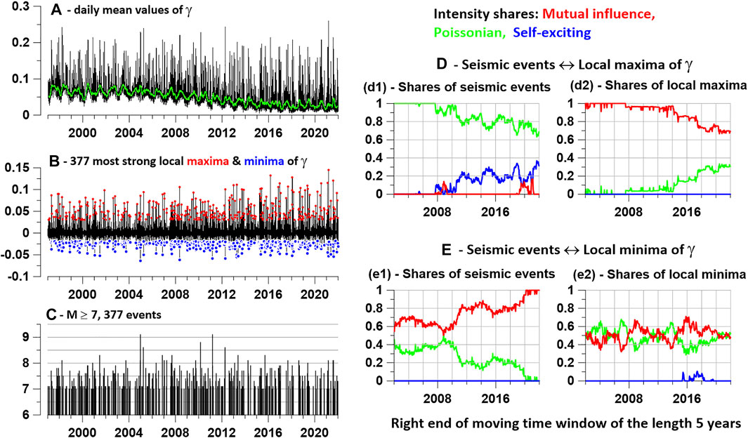
FIGURE 2. (A)—graph of daily average values of the index $\gamma$ calculated for all reference points, green line - moving average in a window of 57 days; (B)—graph of average values of the index $\gamma$ after removal of local trends by a Gaussian window with a radius of 2 days, red and blue dots indicate the 377 most pronounced local maxima and minima of the DJ index $\gamma$ after detrending; (C)—the time sequence of 377 earthquakes with a magnitude of at least 7 for the whole world for the time interval 1997–2021; (D) and (E)—pairs of graphs representing the shares of intensities of sequences of seismic events [(d1) and (e1)] and points of local extrema of the DJ index [(d2) and (e2)] when estimating the model of mutual influence of 2 point processes in a window of 5 years for the relaxation time $\tau$ 15 days.

Graphs 2 (e1) and 2 (e2) describe changes in intensity shares when considering the interaction of a pair of “seismic events”—“minima $\gamma$ ". In Figure 2e1, the red line represents the change in the proportion of the intensity of the “influence” of the minimum points of $\gamma$ on seismic events, and we see that this influence is very significant, and it grows with time and for several finite time windows of 5 years is actually equal to one. Thus, to a large extent, local minima precede seismic events.

The analysis, the results of which are presented in Figure 2, was carried out for local extrema of the singularity spectrum support width $\text{Δ}\alpha$ and the minimum entropy $En$. The results of obtaining estimates of the degree of influence of minima $\Delta \alpha$ and maxima $En$ on the sequence of seismic events are shown in Figure 3 by the purple and blue lines. At the same time, the red line in Figure 3 shows the proportion of intensity corresponding to the influence of local minima $\gamma$ (red line in Figure 2e1).

FIGURE 3

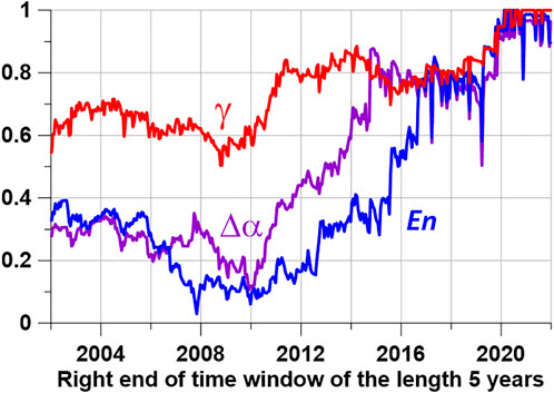
FIGURE 3. Intensity shares corresponding to the “excitation” of seismic events $M\ge 7$ by local extrema of average daily values of seismic noise properties: DJ-index $\gamma$ minima (red line), singularity spectrum support width $\Delta \alpha$ minima (purple line), normalized entropy $En$ maxima (blue line).

A notable feature of the graphs in Figure 3 is the simultaneous reaching of the maximum value equal to 1 for all curves describing the “prognostic power” of local extrema of the seismic noise properties under study. Taking into account the fact that the length of the time window is 5 years, the time interval during which the “predictive power” of all 3 properties reached its maximum takes the time interval 2015–2021. At the same time, the DJ-index $\gamma$ demonstrates the strongest predictive abilities.

Maps of Noise Properties and Distribution of Their Extreme Values

Having values at 50 points distributed around the world makes it possible to map the spatial distribution of seismic noise properties. To build a map, consider a regular grid of 50 nodes in latitude and 100 nodes in longitude, covering the entire earth’s surface. Let ${\zeta }_k,k=1,\mathrm{...},m$ be the coordinates of the reference points (in our case, $m=50$), $Z_k$ are the values of one or another property of the noise at the reference point $\#k$, $r$ is the coordinates of node of the regular grid, $d\left({\zeta }_k,r\right)$ is the distance along the surface of the spherical Earth between the points ${\zeta }_k$ and $r$, $h$ is the bandwidth (smoothing radius) of Gaussian kernel function. Then the values at the nodes of the regular grid are calculated using the Nadaraya-Watson formula (Duda et al., 2000):

$\widehat{Z}\left(r\right)={\displaystyle \sum _{k=1}^m{Z}_k\exp \left(-d^2\left({\zeta }_k,r\right)/h^2\right)}/{\displaystyle \sum _{k=1}^m\exp \left(-d^2\left({\zeta }_k,r\right)/h^2\right)}(26)$

The smoothing radius $h={15}^{\circ }$ was used, which corresponds to a distance of near 1700 km. Values $\widehat{Z}\left(r\right)$ calculated daily at all nodes $r$ make it possible to obtain daily distribution maps over the space of seismic noise properties. The result of averaging all daily charts between some 2 dates gives the corresponding average map.

Consider the values of the noise property as a function of two-dimensional vectors $z_{ij}=\left(x_i,y_j\right)$ of longitudes and latitudes of nodes $\left(i,j\right)$ in an explicit form: $U_{ij}^{\left(t\right)}\equiv U^{\left(t\right)}\left(z_{ij}\right)$. For each daily “elementary chart” with a discrete time index $t$, we find the coordinates of nodes $z_{mn}^{\left(t\right)}=\left(x_m^{\left(t\right)},y_n^{\left(t\right)}\right)$, at which extreme values of $U$ are reached with respect to all other nodes of the regular grid. If $U=\Delta \alpha$ or $U=\gamma$ , then they will look for the minimum values, and if $U=En$, then they will look for the maximum values. A cloud of two-dimensional vectors $z_{mn}^{\left(t\right)}$ considered within a certain time interval $t\in \left[t_0,t_1\right]$ forms a random set. Let us estimate their two-dimensional probability distribution function for each node $z_{ij}$ of the regular grid. For this, the Parzen–Rosenblatt estimate with the Gaussian kernel function (Duda et al., 2000) will be applied:

$p\left(z_{ij}|t_0,t_1\right)=\frac{1}{2\pi h^2\left(t_1-t_0+1\right)}{\displaystyle \sum _{t=t_0}^{t_1}{\displaystyle \sum _{mn}\exp \left(-\frac{|z_{ij}-z_{mn}^{\left(t\right)}{|}^2}{2h^2}\right)}}(27)$

Here $h$ is the kernel averaging radius, $t_0,t_1$ are integer indices that number the daily “elementary” maps. Thus, $\left(t_1-t_0+1\right)$ is the number of daily charts in the considered time interval. The smoothing bandwidth $h={15}^{\circ }$ was used.

Figure 4 shows the average maps of the distribution of 3 properties of seismic noise, obtained by interpolating the values from the reference points to the entire surface of the Earth using formula (15), as well as maps of the probability density distribution of extreme values calculated using formula (16). It can be seen that the distributions of noise property values are strongly correlated with each other. In this case, it should be taken into account that the maxima of $En$ correspond to the minima $\Delta \alpha$ and $\gamma$. The correlation coefficients $r$ between the averaged digital maps in the left column of the maps in Figure 4 are: $r\left(\gamma ,\text{Δ}\alpha \right)=\text{0}\text{.}9684$, $r\left(En,\text{Δ}\alpha \right)=-\text{0}\text{.}8907$, $r\left(En,\gamma \right)=-\text{0}\text{.}9040$. In the right column of digital maps in Figure 4, all correlations are positive and for the same sequence of property pairs are 0.7640, 0.7509, and 0.8991.

FIGURE 4

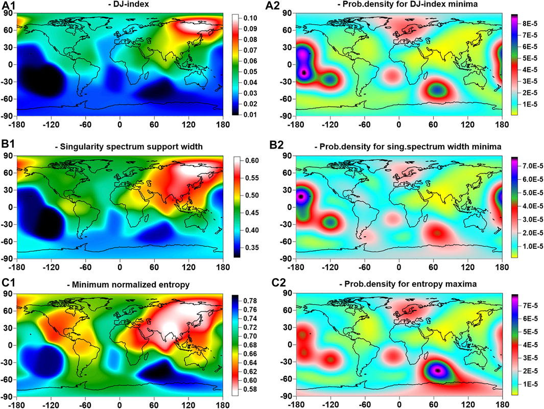
FIGURE 4. On the left—(A1–C1)—` averaged maps of the distribution of seismic noise parameters $\gamma$, $\Delta \alpha$ and $En$, obtained by interpolation of values from the network of reference points using a Gaussian kernel with an averaging window radius of 15°; on the right—(A2–C2)—probability density maps of the distribution of extreme values (minima for $\gamma$ and $\Delta \alpha$, maxima for $En$), also obtained using a Gaussian kernel with a smoothing radius of 15°.

Coherence Spectra

For the further analysis it is necessary to estimate coherence spectra between 2 time series within sliding time window. A parametric model of vector autoregression will be used which provides a better frequency resolution with respect to methods of spectra and cross-spectra estimates based on Fourier expansion (Marple, 1987). For the multiple time series $X\left(t\right)$ of dimensionality $q$ AR-model is defined by a formula:

$X\left(t\right)+{\displaystyle \sum _{k=1}^p{B}_k\cdot }X\left(t-k\right)=\epsilon \left(t\right)(28)$

Here $t$ is a discrete time index, $p$ is autoregression order, $B_k$ are matrices of autoregression coefficients of the size $q\times q$, $P=M\left\{\epsilon \left(t\right){\epsilon }^T\left(t\right)\right\}$ is covariance matrix of the size $q\times q$ of residual signal $\epsilon \left(t\right)$. Matrices $B_k$ and $P$ are computed by Durbin-Levinson procedure (Marple, 1987). Parametric estimate of spectral matrix is defined by the formula:

$S_{XX}\left(\omega \right)={\text{Φ}}^{-1}\left(\omega \right)\cdot P\cdot {\text{Φ}}^{-H}\left(\omega \right),\mathrm{\Phi }\left(\omega \right)=E+{\displaystyle \sum _{k=1}^p{B}_k}{e}^{-i\omega k}(29)$

where $E$ is a unit matrix of the size $q\times q$. For dimensionality $q=2$ coherence spectrum is computed by the formula:

$\lambda \left(\omega \right)=\left|S_{12}\left(\omega \right)\right|/\sqrt{S_{11}\left(\omega \right)\cdot S_{22}\left(\omega \right)}(30)$

Here $S_{11}\left(\omega \right)$ and $S_{22}\left(\omega \right)$ are diagonal elements of the matrix 29) whereas $S_{12}\left(\omega \right)$ is cross-spectrum.

First Principal Components at Reference Points and Maximum Coherences

As follows from the distribution maps of noise properties and their extreme values in Figure 4, the behavior of these properties has much in common, but there are also individual differences. To extract the common components of noise properties, we calculate the first principal component of 3 properties $\left(\gamma ,\Delta \alpha ,En\right)$ at each reference point according to formulas (10-13) in a sliding time window 365 days long. Next, we study the variability in time and space of coherences between the values of the first principal components of noise properties at all nodes of the reference points network. To calculate the pairwise coherence functions between the values of the first principal components at the reference points, we used the 2nd order vector autoregression model (28) with a preliminary transition to increments. The choice of a low order of autoregression pursued the goal of suppressing random fluctuations in the coherence estimates and obtaining smooth frequency dependences. The calculations were made in sliding time windows 365 days long with a shift of 3 days. The use of coherence spectra instead of correlation coefficients (Lyubushin, 2020c) makes it possible to obtain higher measures of connectivity between noise property values at reference points by choosing the frequencies at which the maximum values are realized.

Let ${\mu }_{ij}^{\left(\tau \right)}$ be the maximum with respect to frequencies of the coherence function between the values of the principal components at the reference points with numbers $i$ and $j$ for the window with the time stamp $\tau$ of the right end. Calculate the average values for all pairs of reference points $\overline{\mu }\left(\tau \right)={\displaystyle {\sum }_{\left(i,j\right)}{\mu }_{ij}^{\left(\tau \right)}}/M$, where $M=m\left(m-1\right)/2$ is the number of different pairs of reference points from their total number. In our case $m=50$, $M=1225$. We extract those pairs of reference points for which the maximum coherence ${\mu }_{ij}^{\left(\tau \right)}$ in the current time window $\tau$ exceeded the threshold of 0.8 and denote by $n\left(\tau \right)$ the total number of such pairs in each time window, and by $\rho \left(\tau \right)$ the average distance between such reference points. The threshold 0.8 for maximum coherence value is considered as a large enough one for extracting strong linear frequency-depended connection between seismic noise properties in different reference points. Dependences $\overline{\mu }\left(\tau \right)$, $n\left(\tau \right)$ and $\rho \left(\tau \right)$ are shown in Figure 5.

FIGURE 5

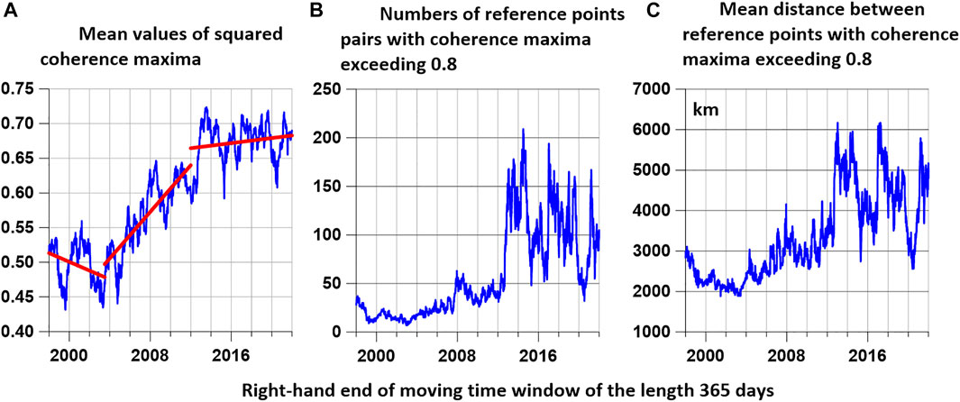
FIGURE 5. (A)—plot of the mean values of the quadratic coherence maxima between the values of the first principal component of the 3 seismic noise properties in all pairs of the network of 50 reference points on the Earth’s surface estimated in a sliding time window of 365 days with a shift of 3 days, the red lines represent linear trends on the time intervals of the right ends of the window 1998–2003.5, 2003.5–2012 and 2012–2022. (B) is a graph of the number of pairs of reference points for which the maximum coherence exceeded the threshold of 0.8. (C) is the graph of mean distance between reference points with high maximum squared coherence.

In the dependence $\overline{\mu }\left(\tau \right)$ on Figure 5A, attention is drawn to the break in the trend in the vicinity of the time point of the right end of the annual window 2003.5. This feature is highlighted by linear trend red lines built before and after mid-2003. After 2003.5, a rapid increase in the average maximum coherence began. This time point of a break in the trend has already been found for the behavior of the average value of the absolute values of pairwise correlations, estimated in a sliding time window of 365 days, for other daily properties of seismic noise (Lyubushin, 2020a; Lyubushin, 2020c; Lyubushin, 2021c). As a reason for the change in the trend of the correlation of seismic noise properties in these works, a hypothesis was proposed about the triggering effect of a high-frequency anomaly in the Earth’s rotation regime, which can also be the cause of an increase in the intensity of the strongest earthquakes in the world after the Sumatran mega-earthquake on 26 December, 2004. In Figures 5B,C, for the number $n\left(\tau \right)$ of pairs of reference points with strong coherence and for the mean distances $\rho \left(\tau \right)$ between such points, after the time right point of the annual window 2012, the regime of high-frequency chaotic fluctuations with high amplitude begins. At the same time, at the time point of 2012, there is another change in the trend in the behavior of the average maximum coherence $\overline{\mu }\left(\tau \right)$ in Figure 5A. The appearance of another characteristic time point in the behavior of seismic noise is presumably associated with the destabilization of the noise field after two mega earthquakes close in time: 27 February 2010, M = 8.8 in Chile and 11 March 2011, M = 9.1 in Japan (Lyubushin, 2020c; Lyubushin, 2021c).

Mean Correlations Between Seismic Noise Properties

Besides the analysis of first principal components of seismic noise properties, their correlation can also be used to extract the hidden general features of seismic noise behavior. Since the property values are tied to a network of reference points, it becomes possible to calculate at each point the average values of absolute pairwise correlations between daily values $\left(\gamma ,\mathrm{\Delta }\alpha ,En\right)$ in a sliding time window of a certain length and then analyze the distribution of the maximum values of these correlations both in space and in time. As before, a time window of 365 days was used. The results of the analysis of correlations are presented in Figure 6. Figures 6A,B show the average maps of the distribution of the maximum values of the mean absolute correlations over space, calculated using the kernel estimate (16) for the annual time windows located before and after 2012. Figures 6C,D show graphs of changes in coordinates (geographical longitude and latitude) of points on the Earth’s surface, in which the maximum values of average absolute correlations were realized for each position of the time window.

FIGURE 6

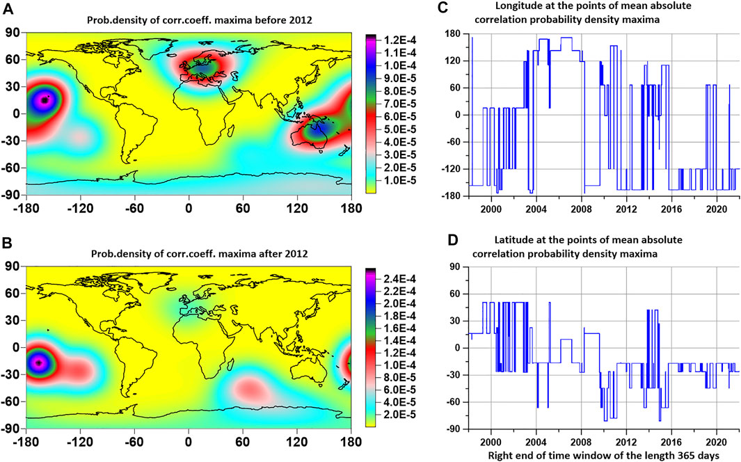
FIGURE 6. (A,B) are maps of probability density distributions of the maxima of the average values of the modules of pairwise correlation coefficients between the values of seismic noise properties $\gamma$, $\Delta \alpha$ and $En$ at each reference point in a sliding time window 365 days long for the timestamps of the right end of the window before and after 2012. (C,D) are plots of longitude and latitude of points of maximum probability densities of maximum values of average absolute correlations of noise properties.

It can be seen from the distribution of maximum correlation values in Figures 6A,B that the maxima are concentrated mainly in the western part of the Pacific Ocean, and after 2012 the points of maximum correlations completely shifted to the Southern Hemisphere, and after 2016 they were mainly concentrated in the region islands of Tonga, where the largest volcanic eruption Hunga Tonga-Hunga Ha’apai occurred on 15 January, 2022 (Poli and Shapiro, 2022).

Relationship Between the Properties of Seismic Noise and Irregular Rotation of the Earth

The uneven rotation of the Earth is mainly explained by the influence of processes in the atmosphere (Zotov et al., 2017). At the same time, some researchers pointed to a connection between the irregular rotation of the Earth and seismicity (Shanker et al., 2001; Levin et al., 2017). A possible trigger mechanism for the influence of Earth rotation variations on the seismic process was studied in (Bendick, and Bilham, 2017). Estimates of the impact of a strong earthquake on the length of the day are given in (Xu and Sun, 2012). Length of day (LOD) data are available from the website at: https://hpiers.obspm.fr/iers/eop/eopc04/eopc04.62-now.

The maximum quadratic coherences between the LOD and the first principal components of the seismic noise properties at each reference point were estimated. The coherences were evaluated in sliding time windows of 365 days with a shift of 3 days using a 5th order vector (two-dimensional) autoregressive model. Similar DJ-index response estimates distributed over the Earth’s surface in a network of reference points were previously used in (Lyubushin, 2021c). Figure 7 shows examples of graphs of the maximum quadratic coherence between the first principal components at three reference points with numbers 4, 20, and 34 (the same as in Figure 1) and LOD.

FIGURE 7

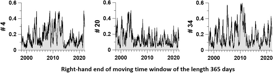
FIGURE 7. Plots of maximum values of quadratic coherences between day length LOD and the first principal component of 3 seismic noise properties $\gamma$, $\Delta \alpha$ and $En$ at 3 reference points numbered 4, 20 and 34 when estimating in a sliding time window of 365 days with a 3 day offset.

Figure 8 shows graphs of two synchronous curves: Figure 8A shows the logarithm of the released seismic energy (in joules) in a sequence of time intervals 365 days long, taken with a shift of 3 days; Figures 8B—average values of maximum coherences between time series of LOD and daily values of the first components of noise properties at 50 control points. The behavior of the curve in Figure 8B can be divided into 3 sections. The first 2 time stamps of the right ends of the windows before and after 2012 differ significantly from each other in the average values represented by the horizontal red lines. The final section is due to the most recent data (orange line) and it is characterized by abnormal spike. Note that the behavior of the average maximum pairwise coherences exceeding the threshold of 0.8 in Figure 5B is also very different for the timestamps of the right ends of the windows before and after 2012. Thus, the response of seismic noise properties to the irregularity of the Earth’s rotation turned out to be dependent on the degree of spatial connectivity of strong coherences of noise properties.

FIGURE 8

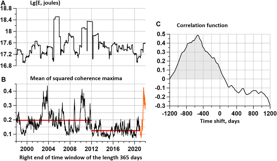
FIGURE 8. (A)—plot of the values of the decimal logarithm of the released seismic energy (joules) in a sliding time window 365 days long with a shift of 3 days; (B)—the black line represents the average of the quadratic coherence maxima between the LOD and the first principal component of the 3 seismic noise properties in a 365-day window with a 3-day offset for the positions of the right end of the time window in the interval 1998–2021, the red horizontal lines represent the average coherence values for time intervals 1998–2012 and 2012–2021. The orange line in Figure (B) represents the plot of the mean coherence for the positions of the right end of the time window in the interval 2021–2022. The plot in Figure (C) represents the correlation function between the logarithm of the released seismic energy and the mean quadratic coherence for time shifts of ±1200 days. A strong shift of the correlation function plot towards negative time shifts with a maximum for a shift of -530 days confirms the hypothesis that bursts of coherence between LOD and seismic noise properties precede seismic energy releases with a delay of about 1.5 years.

The third time interval is represented by the orange line and relates to the processing of the most recent time-stamped right end windows after 2021, then referring to the time span of 2020–2021. The selection of a short 3rd segment based on the results of data processing in 2021 is due to an unusually large burst in the response of noise properties to LOD. An additional intrigue to the occurrence of this burst is introduced by the estimation of the correlation function between the logarithm of the released seismic energy in Figure 8A and the average maximum coherence between the noise and LOD properties in the GCP network in Figure 8B, represented by the plot in Figure 8C) for time shifts of ±1200 days. The correlation function has a significant asymmetry and is shifted to the area of negative time shifts, which correspond to the advance of the coherence maxima of the seismic energy emission maxima. The maximum correlation falls on a time shift of -530 days. This estimate of cross-correlations suggests that the burst represented by the orange lines in Figure 8B may precede a major earthquake with an average delay of 1.5 years.

Although the value of correlation near 0.5 is rather small and it could not be an argument for statistically significant linear connection between 2 random variables, I suppose that main purpose of correlation function estimate is establishing the fact that one variable is shifted with respect to other. The strong asymmetry of correlation function at Figure 8C confirms preceding of coherence burst to burst of seismic energy which could be noticed visually by comparing graphs at Figures 8A,B.

Discussion

The main result of the article is that since 2003 there has been an increase in the global seismic hazard, and in the process of this increase, attention should be paid to the phenomena characteristic of the last annual time windows. First of all, these are graphs of the behavior of the “prognostic forces” of the points of local extrema of the analyzed properties of seismic noise in relation to the sequence of the strongest earthquakes in Figure 3. This figure shows that for all analyzed noise properties, the graphs of their predictive power reached the maximum value equal to 1. The graphs in Figure 3 show that the DJ index $\gamma$ has the highest predictive power compared to the singularity spectrum support width $\Delta \alpha$ and entropy $En$ over all 25 years of observation. However, in the final time intervals of 2015–2021 the predictive power of all noise properties became equal, and it became difficult to make a choice in the direction of the “best” property of seismic noise. Therefore, a choice was made in favor of a joint analysis of all 3 properties using the principal component method in a sliding time window.

In addition, a strong spike in mean maximum coherence values between the principal components of the seismic noise properties in the network of reference points and the LOD time series represented by the orange line in Figure 8B is a sign of increasing current hazard. Visually, when comparing the graphs in Figures 8A,B, it is noticeable that bursts of coherence precede seismic energy emissions, which is confirmed by the evaluation of the correlation function in Figure 8C.

Summarizing, we can distinguish two critical time intervals when the properties of seismic noise have changed significantly. Considering that the properties of seismic noise are estimated in sliding time windows of 365 days, the critical time intervals are also determined with an accuracy of 1 year.

The first time interval 2002.5–2003.5 refers to the change in the trend of the average maximum coherence between the values of the first components of the noise properties at the reference points. After this interval, a systematic increase in the average maximum coherence is observed (Figure 5A), which is superimposed by periodic fluctuations with a period of about 1000 days. The second critical time interval in the behavior of global seismic noise refers to 2011–2012. After it, chaotic pulsations begin with a high amplitude of change in the number of pairs of reference points and average distances between reference points, for which a strong pairwise coherence has arisen that exceeds the threshold of 0.8 (Figures 5B,C).

Estimating the place of seismic hazard concentration by studying the properties of seismic noise, according to the method used, is reduced to determining the places where extreme values are most often observed, that is, to assessing the spatial distribution densities of the minima for $\gamma$, $\Delta \alpha$, and the maxima for $En$. Such estimates are shown in the maps in the right column in Figure 4. As already noted, these digital maps are highly correlated, and attention should be paid to the region in the west and in the center of the Pacific Ocean. Another way to assess seismic hazard locations is to estimate the distribution density of the maximum values of the average absolute correlations between noise properties, shown in Figures 6A,B. However, one should keep in mind the low density of seismic stations, especially in oceanic areas in the Southern Hemisphere, as a result of which the estimates of the distribution of extreme values of noise properties are subject to strong uncertainty.

It should be noticed that the used data analysis technique has a lot of common features with method of investigating properties of high-frequency seismic noise in Central Italy before L’Aquila earthquake in 2009 such as using spectral matrices and entropy of spectral matrices eigenvalues (Shi et al., 2020). The main differences consist in frequency range and in using nonlinear transform from initial seismic records to their properties (wavelet-based minimum entropy, DJ-index and multi-fractal singularity spectrum support width) estimated within adjacent daily time intervals.

Conclusion

In this paper, a phenomenological approach is applied to the study of complex multicomponent systems, which include the earth’s crust, based on the general property of an increase in the radius and degree of strong coherence of random fluctuations in the parameters of a complex system as it approaches a sharp change in its properties, as a result of its own dynamics. As a result of the study of long-term continuous recordings of low-frequency seismic noise on a network of broadband seismic stations covering the entire globe, it was possible to establish characteristic time points for changing trends in the coherence of seismic noise properties and to determine the relationship between changes in these properties and the uneven rotation of the Earth.

Data Availability Statement

Publicly available datasets were analyzed in this study. This data can be found here: Incorporated Research Institutions for Seismology (IRIS) website at http://www.iris.edu/forms/webrequest/from 229 broadband seismic stations of 3 networks: http://www.iris.edu/mda/_GSN, http://www.iris.edu/mda/G, http://www.iris.edu/mda/GE INTERNATIONAL EARTH ROTATION AND REFERENCE SYSTEMS SERVICE, https://hpiers.obspm.fr/iers/eop/eopc04/eopc04.62-now.

Author Contributions

The author confirms being the sole contributor of this work and has approved it for publication.

Conflict of Interest

The author declares that the research was conducted in the absence of any commercial or financial relationships that could be construed as a potential conflict of interest.

Publisher’s Note

All claims expressed in this article are solely those of the authors and do not necessarily represent those of their affiliated organizations, or those of the publisher, the editors and the reviewers. Any product that may be evaluated in this article, or claim that may be made by its manufacturer, is not guaranteed or endorsed by the publisher.

Acknowledgments

The work was carried out within the framework of the state assignment of the Institute of Physics of the Earth of the Russian Academy of Sciences.

References

Ardhuin, F., Stutzmann, E., Schimmel, M., and Mangeney, A. (2011). Ocean Wave Sources of Seismic Noise. J. Geophys. Res. 116, C09004. doi:10.1029/2011jc006952

CrossRef Full Text | Google Scholar

Aster, R. C., McNamara, D. E., and Bromirski, P. D. (2008). Multidecadal Climate-Induced Variability in Microseisms. Seismol. Res. Lett. 79, 194–202. doi:10.1785/gssrl.79.2.194

CrossRef Full Text | Google Scholar

Bendick, R., and Bilham, R. (2017). Do weak Global Stresses Synchronize Earthquakes? Geophys. Res. Lett. 44, 8320–8327. doi:10.1002/2017gl074934

CrossRef Full Text | Google Scholar

Chandrasekhar, E., Prabhudesai, S. S., Seemala, G. K., and Shenvi, N. (2016). Multifractal Detrended Fluctuation Analysis of Ionospheric Total Electron Content Data during Solar Minimum and Maximum. J. Atmos. Sol.-Terr. Phys. 149, 31–39. doi:10.1016/j.jastp.2016.09.007

CrossRef Full Text | Google Scholar

Costa, M., Goldberger, A. L., and Peng, C. K. (2005). Multiscale Entropy Analysis of Biological Signals. Phys. Rev. E Stat. Nonlin Soft Matter Phys. 71, 021906. doi:10.1103/PhysRevE.71.021906

PubMed Abstract | CrossRef Full Text | Google Scholar

Costa, M., Peng, C.-K., Goldberger, A. L., and Hausdorff, J. M. (2003). Multiscale Entropy Analysis of Human Gait Dynamics. Phys. A Stat. Mech. its Appl. 330, 53–60. doi:10.1016/j.physa.2003.08.022

CrossRef Full Text | Google Scholar

Cox, D. R., and Lewis, P. A. W. (1966). The Statistical Analysis of Series of Events. London: Methuen.

Google Scholar

Currenti, G., del Negro, C., Lapenna, V., and Telesca, L. (2005). Multifractality in Local Geomagnetic Field at Etna Volcano, Sicily (Southern Italy). Nat. Hazard. Earth Syst. Sci. 5, 555–559. doi:10.5194/nhess-5-555-2005

CrossRef Full Text | Google Scholar

Donoho, D. L., and Johnstone, I. M. (1995). Adapting to Unknown Smoothness via Wavelet Shrinkage. J. Am. Stat. Assoc. 90 (432), 1200–1224. Available at: http://statweb.stanford.edu/∼imj/WEBLIST/1995/ausws.pdf. doi:10.1080/01621459.1995.10476626

CrossRef Full Text | Google Scholar

Duda, R. O., Hart, P. E., and Stork, D. G. (2000). Pattern Classification. New York, Chichester, Brisbane, Singapore, Toronto: Wiley-Interscience Publication.

Google Scholar

Feder, J. (1988). Fractals. New York, London: Plenum Press.

Google Scholar

Gilmore, R. (1981). Catastrophe Theory for Scientists and Engineers. New York, NY: John Wiley & Sons, 666.

Google Scholar

Hardle, W. (1990). Applied Nonparametric Regression. (Biometric Society Monographs No. 19.). Cambridge: Cambridge University Press.

Google Scholar

Ida, Y., Hayakawa, M., Adalev, A., and Gotoh, K. (2005). Multifractal Analysis for the ULF Geomagnetic Data during the 1993 Guam Earthquake. Nonlin. Process. Geophys. 12, 157–162. doi:10.5194/npg-12-157-2005

CrossRef Full Text | Google Scholar

Ivanov, P. C., Amaral, L. A., Goldberger, A. L., Havlin, S., Rosenblum, M. G., Struzik, Z. R., et al. (1999). Multifractality in Human Heartbeat Dynamics. Nature 399, 461–465. doi:10.1038/20924

PubMed Abstract | CrossRef Full Text | Google Scholar

Jolliffe, I. T. (1986). Principal Component Analysis. New York, NY: Springer-Verlag. doi:10.1007/b98835

CrossRef Full Text | Google Scholar

Kantelhardt, J. W., Zschiegner, S. A., Konscienly-Bunde, E., Havlin, S., Bunde, A., and Stanley, H. E. (2002). Multifractal Detrended Fluctuation Analysis of Nonstationary Time Series. Phys. A Stat. Mech. Appl. 316 (1-4), 87–114. doi:10.1016/s0378-4371(02)01383-3

CrossRef Full Text | Google Scholar

Kedar, S., Longuet-Higgins, M., Webb, F., Graham, N., Clayton, R., and Jones, C. (2008). The Origin of Deep Ocean Microseisms in the North Atlantic Ocean. Proc. R. Soc. A 464, 777–793. doi:10.1098/rspa.2007.0277

CrossRef Full Text | Google Scholar

Kobayashi, N., and Nishida, K. (1998). Continuous Excitation of Planetary Free Oscillations by Atmospheric Disturbances. Nature 395, 357–360. doi:10.1038/26427

CrossRef Full Text | Google Scholar

Koutalonis, I., and Vallianatos, F. (2017). Evidence of Non-extensivity in Earth's Ambient Noise. Pure Appl. Geophys. 174, 4369–4378. doi:10.1007/s00024-017-1669-9

CrossRef Full Text | Google Scholar

Levin, B. W., Sasorova, E. V., Steblov, G. M., Domanski, A. V., Prytkov, A. S., and Tsyba, E. N. (2017). Variations of the Earth's Rotation Rate and Cyclic Processes in Geodynamics. Geodesy Geodyn. 8 (3), 206–212. doi:10.1016/j.geog.2017.03.007

CrossRef Full Text | Google Scholar

Lyubushin, A. A. (2014). Analysis of Coherence in Global Seismic Noise for 1997-2012. Izv. Phys. Solid Earth 50 (3), 325–333. doi:10.1134/s1069351314030069

CrossRef Full Text | Google Scholar

Lyubushin, A. A. (2017). Long-Range Coherence between Seismic Noise Properties in Japan and California before and after Tohoku Mega-Earthquake. Acta Geod. Geophys 52, 467–478. doi:10.1007/s40328-016-0181-5

CrossRef Full Text | Google Scholar

Lyubushin, A. A., and Pisarenko, V. F. (1994). Research on Seismic Regime Using Linear Model of Intensity of Interacting Point Processes. Izv. Phys. Solid Earth 29, 1108–1113.

Google Scholar

Lyubushin, A. A. (2015). Wavelet-Based Coherence Measures of Global Seismic Noise Properties. J. Seismol. 19 (2), 329–340. doi:10.1007/s10950-014-9468-6

CrossRef Full Text | Google Scholar

Lyubushin, A. (2020b). Connection of Seismic Noise Properties in Japan and California with Irregularity of Earth's Rotation. Pure Appl. Geophys. 177, 4677–4689. doi:10.1007/s00024-020-02526-9

CrossRef Full Text | Google Scholar

Lyubushin, A. (2020c). Global Seismic Noise Entropy. Front. Earth Sci. 8, 611663. doi:10.3389/feart.2020.611663

CrossRef Full Text | Google Scholar

Lyubushin, A. (2021c). Global Seismic Noise Wavelet-Based Measure of Nonstationarity. Pure Appl. Geophys. 178, 3397–3413. doi:10.1007/s00024-021-02850-8

CrossRef Full Text | Google Scholar

Lyubushin, A. (2013). How Soon Would the Next Mega-Earthquake Occur in Japan? Nat. Sci. 5 (8A1), 1–7. doi:10.4236/ns.2013.58A1001

CrossRef Full Text | Google Scholar

Lyubushin, A. (2021b). Low-Frequency Seismic Noise Properties in the Japanese Islands. Entropy 23, 474. doi:10.3390/e23040474

PubMed Abstract | CrossRef Full Text | Google Scholar

Lyubushin, A. (2010). “Multifractal Parameters of Low-Frequency Microseisms,” in Synchronization and Triggering: From Fracture to Earthquake Processes. GeoPlanet: Earth and Planetary Sciences 1. Editors V. de Rubeis, Z. Czechowski, and R. Teisseyre (Berlin Heidelberg: Springer-Verlag), 253–272. Chapter 15. doi:10.1007/978-3-642-12300-9_15

CrossRef Full Text | Google Scholar

Lyubushin, A. (2012). Prognostic Properties of Low-Frequency Seismic Noise. Nat. Sci. 04, 659–666. doi:10.4236/ns.2012.428087

CrossRef Full Text | Google Scholar

Lyubushin, A. (2021a). Seismic Noise Wavelet-Based Entropy in Southern California. J. Seismol. 25, 25–39. doi:10.1007/s10950-020-09950-3

CrossRef Full Text | Google Scholar

Lyubushin, A. (2018). “Synchronization of Geophysical Field Fluctuations,” in Complexity of Seismic Time Series: Measurement and Applications. Editors T. Chelidze, L. Telesca, and F. Vallianatos (Amsterdam, Oxford, Cambridge: Elsevier 2018), 161–197. Chapter 6. doi:10.1016/b978-0-12-813138-1.00006-7

CrossRef Full Text | Google Scholar

Lyubushin, A. (2020a). Trends of Global Seismic Noise Properties in Connection to Irregularity of Earth's Rotation. Pure Appl. Geophys. 177, 621–636. doi:10.1007/s00024-019-02331-z

CrossRef Full Text | Google Scholar

Mallat, S. (1999). A Wavelet Tour of Signal Processing. Second edition. San Diego, London, Boston, New York, Sydney, Tokyo, Toronto: Academic Press.

Google Scholar

Marple, S. L. (1987). Digital Spectral Analysis with Applications. Englewood Cliffs, New Jersey: Prentice-Hall.

Google Scholar

Nicolis, G., and Prigogine, I. (1989). Exploring Complexity, An Introduction. New York, NY: W.H. Freedman and Co., 328.

Google Scholar

Nishida, K., Kawakatsu, H., Fukao, Y., and Obara, K. (2008). Background Love and Rayleigh Waves Simultaneously Generated at the Pacific Ocean Floors. Geophys. Res. Lett. 35, L16307. doi:10.1029/2008gl034753

CrossRef Full Text | Google Scholar

Nishida, K., Montagner, J.-P., and Kawakatsu, H. (2009). Global Surface Wave Tomography Using Seismic Hum. Science 326 (5949), 112. doi:10.1126/science.1176389

PubMed Abstract | CrossRef Full Text | Google Scholar

Pandey, A. P., Singh, A. P., Bansal, B. K., Suresh, G., and Prajapati, S. K. (2020). Appraisal of Seismic Noise Scenario at National Seismological Network of India in COVID-19 Lockdown Situation. Geomatics Nat. Hazards Risk 111, 2095–2122. doi:10.1080/19475705.2020.1830187

CrossRef Full Text | Google Scholar

Pavlov, A. N., and Anishchenko, V. S. (2007). Multifractal Analysis of Complex Signals. Phys. Usp. 50 (8), 819–834. doi:10.1070/pu2007v050n08abeh006116

CrossRef Full Text | Google Scholar

Poli, P., and Shapiro, N. M. (2022). Rapid Characterization of Large Volcanic Eruptions: Measuring the Impulse of the Hunga Tonga Ha’apai Explosion from Teleseismic Waves. Geophys. Res. Lett. 49 (8), e2022GL098123. doi:10.1029/2022GL098123

CrossRef Full Text | Google Scholar

Ramírez-Rojas, A., Muñoz-Diosdado, A., Pavía-Miller, C. G., and Angulo-Brown, F. (2004). Spectral and Multifractal Study of Electroseismic Time Series Associated to the Mw=6.5 Earthquake of 24 October 1993 in Mexico. Nat. Hazards Earth Syst. Sci. 4, 703–709. doi:10.5194/nhess-4-703-2004

CrossRef Full Text | Google Scholar

Rhie, J., and Romanowicz, B. (2004). Excitation of Earth's Continuous Free Oscillations by Atmosphere-Ocean-Seafloor Coupling. Nature 431, 552–556. doi:10.1038/nature02942

PubMed Abstract | CrossRef Full Text | Google Scholar

Sarlis, N. V., Skordas, E. S., Varotsos, P. A., Nagao, T., Kamogawa, M., and Uyeda, S. (2015). Spatiotemporal Variations of Seismicity before Major Earthquakes in the Japanese Area and Their Relation with the Epicentral Locations. Proc. Natl. Acad. Sci. U. S. A. 112, 986–989. doi:10.1073/pnas.1422893112

PubMed Abstract | CrossRef Full Text | Google Scholar

Shanker, D., Kapur, N., and Singh, V. P. (2001). On the Spatio Temporal Distribution of Global Seismicity and Rotation of the Earth - A Review. Acta Geod. Geoph. Hung. 36, 175–187. doi:10.1556/ageod.36.2001.2.5

CrossRef Full Text | Google Scholar

Shi, P., Seydoux, L., and Poli, P. (2020). Unsupervised Learning of Seismic Wavefield Features: Clustering Continuous Array Seismic Data during the 2009 L’Aquila Earthquake. J. Geophys. Res. Solid Earth 126, e2020JB020506. doi:10.1029/2020JB020506

CrossRef Full Text | Google Scholar

Tanimoto, T. (2001). Continuous Free Oscillations: Atmosphere-Solid Earth Coupling. Annu. Rev. Earth Planet. Sci. 29, 563–584. doi:10.1146/annurev.earth.29.1.563

CrossRef Full Text | Google Scholar

Tanimoto, T. (2005). The Oceanic Excitation Hypothesis for the Continuous Oscillations of the Earth. Geophys. J. Int. 160, 276–288. doi:10.1111/j.1365-246X.2004.02484.x

CrossRef Full Text | Google Scholar

Telesca, L., Colangelo, G., and Lapenna, V. (2005). Multifractal Variability in Geoelectrical Signals and Correlations with Seismicity: A Study Case in Southern Italy. Nat. Hazards Earth Syst. Sci. 5, 673–677. doi:10.5194/nhess-5-673-2005

CrossRef Full Text | Google Scholar

Vallianatos, F., Koutalonis, I., and Chatzopoulos, G. (2019). Evidence of Tsallis Entropy Signature on Medicane Induced Ambient Seismic Signals. Phys. A Stat. Mech. Appl. 520, 35–43. doi:10.1016/j.physa.2018.12.045

CrossRef Full Text | Google Scholar

Varotsos, P. A., Sarlis, N. V., and Skordas, E. S. (2003b). Attempt to Distinguish Electric Signals of a Dichotomous Nature. Phys. Rev. E Stat. Nonlin Soft Matter Phys. 68, 031106. doi:10.1103/PhysRevE.68.031106

PubMed Abstract | CrossRef Full Text | Google Scholar

Varotsos, P. A., Sarlis, N. V., Skordas, E. S., and Lazaridou, M. S. (2004). Entropy in the Natural Time Domain. Phys. Rev. E 70 (10), 011106. doi:10.1103/PhysRevE.70.011106

PubMed Abstract | CrossRef Full Text | Google Scholar

Varotsos, P. A., Sarlis, N. V., and Skordas, E. S. (2003a). Long-Range Correlations in the Electric Signals that Precede Rupture: Further Investigations. Phys. Rev. E Stat. Nonlin Soft Matter Phys. 67, 021109. doi:10.1103/PhysRevE.67.021109

PubMed Abstract | CrossRef Full Text | Google Scholar

Varotsos, P. A., Sarlis, N. V., and Skordas, E. S. (2011). “Natural Time Analysis: The New View of Time,” in Precursory Seismic Electric Signals, Earthquakes and Other Complex Time Series (Berlin Heidelberg: Springer-Verlag). doi:10.1007/978-3-642-16449-1

CrossRef Full Text | Google Scholar

Varotsos, P. A., Sarlis, N. V., and Skordas, E. S. (2014). Study of the Temporal Correlations in the Magnitude Time Series before Major Earthquakes in Japan. J. Geophys. Res. Space Phys. 119, 9192–9206. doi:10.1002/2014ja020580

CrossRef Full Text | Google Scholar

Xu, C., and Sun, W. (2012). Co-Seismic Earth's Rotation Change Caused by the 2012 Sumatra Earthquake. Geodesy Geodyn. 3 (4), 28–31. doi:10.3724/SP.J.1246.2012.00028

CrossRef Full Text | Google Scholar

Zotov, L., Sidorenkov, N. S., Bizouard, C., Shum, C. K., and Shen, W. (2017). Multichannel Singular Spectrum Analysis of the Axial Atmospheric Angular Momentum. Geodesy Geodyn. 8 (6), 433–442. doi:10.1016/j.geog.2017.02.010

CrossRef Full Text | Google Scholar