 Ning Qiu
 Zhixin Luo
 Qicheng Fu
 Zhen Sun
 Yanjun Chang4*
- 1Hainan Key Laboratory of Marine Geological Resources and Environment, Haikou/Key Laboratory of Ocean and Marginal Sea Geology, South China Sea Institute of Oceanology, Innovation Academy of South China Sea Ecology and Environmental Engineering, Chinese Academy of Sciences, Guangzhou, China
- 2Southern Marine Science and Engineering Guangdong Laboratory (Guangzhou), Guangzhou, China
- 3College of Ocean and Meteorology, Guangdong Ocean University, Zhanjiang, China
- 4Institute of Geophysics and Geomatics, China University of Geosciences, Wuhan, China
- 5Key Laboratory of Geophysical Electromagnetic Probing Technologies of Ministry of Natural Resources of the People’s Republic of China, Langfang, China
The identification of hydrocarbons buried on the seafloor is highly dependent on geophysical exploration capabilities. Seismic exploration has been an important tool in providing information on submarine stratigraphy before offshore drilling, but it is a challenge to identify the nature and saturation of the fluid in the structure by seismic exploration. Of all the physical properties, electrical parameters are the most sensitive to the fluids in the reservoir and would be able to be combined with seismic data to improve the identification of hydrocarbons at depth. However, the marine controlled-source electromagnetic method usually only considers the effect of electromagnetic induction and ignores the induced polarization (IP) effects. The IP effects can occur in the stratum where the reservoir is located due to a variety of factors, so considering the IP effects will make the modeling more reasonable and thus give more accurate results when interpreting and processing the data. We have used the integral equation method for modeling, adopted the scattering and superposition methods to calculate the dyadic Green’s function required in the study, replaced the real resistivity with a complex resistivity that takes into account the IP effects, investigated the response patterns of different ion polarization models, and analyzed the influence patterns of various model parameters. These investigations will provide important contributions to the study of submarine hydrocarbon detection. The field data also show the amplitude, and phase response results of polarizability show that it gradually increases from the offset.
1 Introduction
The marine geophysical method is one of the most important tools used to explore the structure and resources under the seafloor (Liu et al., 2017). 3D seismic exploration has been an essential approach to providing information on the stratigraphy of the seafloor prior to marine drilling. It is usually desirable to understand the nature of the fluids in the formation through geophysical exploration to improve the success rate of drilling (Xu et al., 2018; Cai et al., 2020; Guo et al., 2021; Liu et al., 2021; Wang et al., 2021; Yu et al., 2022). However, it is challenging to identify the nature and saturation of the fluid in the structure by seismic (Guo et al., 2021). It is noted that of all the physical properties, electrical parameters (resistivity/conductivity and dielectric constant) are the most sensitive to the fluids in the reservoir and would be able to be combined with seismic data to improve the identification of hydrocarbons (HCs) at depth (Strack, 2014). Since the 1970s, marine electromagnetic methods have been recognized and included as a research topic. However, it was not until the 1990s that research on marine electromagnetic methods gradually developed (Nabighian, 1991). The main methods applied in marine exploration are the marine controlled-source electromagnetic method (CSEM) and the marine magnetotelluric method (MT) (Constable, 2013). In particular, CSEM, as a new marine oil and gas exploration technique, has broken the dullness of marine non-seismic exploration and is known as the most important geophysical survey technique since the emergence of 3D reflection seismic survey decades ago. With the development and exploitation of subsea oil and gas resources, CSEM has gradually developed from the initial application of probing the marine environment, geological structures, and mineral resources in the deep sea. It has gradually become an important method for finding subsea oil and gas resources (Constable and Srnka, 2007).
The resistivity of oil and gas reservoirs are usually tens to hundreds of times higher than that of the surrounding rock, so the low resistivity of the surrounding rock and the high resistivity of the oil and gas reservoirs form an obvious diversity in resistivity. Thus, the submarine oil and gas resources can be easily detected by CSEM (Chave and Cox, 1982).
The CSEM exploration technology was developed by ENI-AGIP Petroleum Company. Commercial projects can already be explored. Between 1996 and 2003, Morrison, AOA, California Berkeley, Scripps, and Arnold Orange of Hoversten Geophysical Company conducted a large number of tests in the Gemini work area of the Gulf of Mexico. Statoil was the first to conduct a test of directly detecting offshore oil and gas with MCSEM and achieved success. Constable and Srnka (2007) studied the identification ability of marine CSEM for high-resistivity thin layers. These experimental studies have verified the feasibility of MCSEM in the exploration of submarine oil and gas hydrates. In recent years, companies such as OHM in the United Kingdom, EMGS in Norway, AGO, and MTEM in the United States have completed hundreds of MCSEM exploration projects; most of which have been verified by drilling results (Constable, 2013). At present, breakthroughs have been made in the 1D, 2D, 2.5D, and 3D forward modeling theories of marine CSEM. The Scripps Institute of Oceanography was the first institution to carry out MCSEM forward research. In 1982, Chave studied marine CSEM based on a horizontal electric dipole source in detail. Subsequently, Flosadotir and Constable (1996) introduced the fast Hankel transform algorithm and the Occam smooth inversion algorithm based on their research and completed the research of the 1D forward and inversion programs. Based on Chave’s algorithm, Unsworth and Oldenburg (1995) studied and wrote 2.5D forward and inverse algorithm programs. MacGregor adapted Unsworth’s forward algorithm and introduced the Occam inversion algorithm to calculate the measured data in the work area. Everett studied a time-domain algorithm for the 2.5D model. Bakr et al. (2013) developed a numerical method based on domain decomposition for the simulation of 3D marine CSEM. Zhdanov et al. (2011) developed our implementation of an iterative migration method for CSEM data that is equivalent to rigorous 3D inversion.
However, marine CSEM usually only considers electromagnetic induction but ignores the IP effect. The IP effect can occur in the reservoir due to various factors (Veeken et al., 2009), so considering the IP effect as well will make the modeling more reasonable and therefore give more accurate results when interpreting and processing the data (Veeken et al., 2012; Xu and Sun, 2018). We have used the integral equation method for modeling, adopted the scattering and superposition methods to calculate the dyadic Green’s function required in the study, replaced the real resistivity with a complex resistivity that takes into account the IP effect, investigated the response patterns of different ion polarization models, and analyzed the influence patterns of various model parameters. These investigations will provide important contributions to the study of submarine hydrocarbon detection.
2 Methodology
2.1 Marine controlled-source electromagnetic method
The basic principle of CSEM is electromagnetic induction, where an alternating electric field can induce an alternating magnetic field, and an alternating magnetic field can in turn induce an alternating electric field. Energy is thus constantly transformed in the form of electric and magnetic fields and radiated into space by alternating between the two fields, with the same refraction and reflection occurring when it encounters different media interfaces. When electromagnetic fields propagate through media of various resistivity, they have both similar and different characteristics. The similarity is that, regardless of whether the medium is of high or low resistivity, the energy of electromagnetic waves will be reduced with the distance of propagation in a geometrically attenuated manner; the difference is that high-resistivity media hardly absorb the energy of electromagnetic waves, but low-resistivity media strongly absorb the energy of electromagnetic waves, that is, the existence of “eddy current”. Therefore, it is possible to analyze the received electromagnetic field responses to obtain the electrical distribution of the subsurface medium.
CSEM as a means of identifying HC is that porous rocks are resistive when saturated with natural gas or oil (Fan et al., 2010). For conventional marine CSEM surveys, the horizontal current dipole is used as a source to generate electromagnetic fields and is towed close to the submarine to avoid energy loss in conducting seawater. The receiver is located on the ocean floor. An underground reservoir of higher resistive HC embedded in a conductive background acts as an auxiliary source to direct the electromagnetic field back to the receiver. In this way, one can infer from the measured electromagnetic field that there are resistors underground.
Marine CSEM in oil and gas exploration first processes the data of the measured electric or magnetic field, analyses the electrical distribution of the subsurface medium through processing and interpretation, and then evaluates the hydrocarbon-bearing properties of the highly resistive layer by the relationship between the electrical and physical characteristics of the rock and ore. The resistivity of oil and gas reservoirs is typically in the order of tens to hundreds of ohmmeters, while the resistivity of the overburden above the oil and gas and the sedimentary layers below is typically a few ohmmeters or even less. When an electromagnetic wave propagates through a highly resistive oil layer, the energy decays slowly and travels forward along the reservoir level at a faster rate because the resistivity of the highly resistive layer is greater than that of the surrounding overburden, and the receiving device on the seabed picks up the electromagnetic energy or current that leaks and reflects back from the reservoir level (similar to a seismic refraction wave). MCSEM is used to find oil and gas reservoirs by analyzing the electrical differences between high-resistivity oil layers and low-resistivity surrounding rocks. Depending on the time and frequency domain, the emission source, the observation point, and the observation field, there are various ways of working with CSEM. At present, the most effective method for identifying highly resistive subsurface bodies in domestic and international marine exploration is the frequency domain CSEM, while the transmitting source is a horizontal electric dipole source. Figure 1 shows that the current common working methods of CSEM exploration can be divided into towed receiver point construction methods and fixed receiver point construction methods.
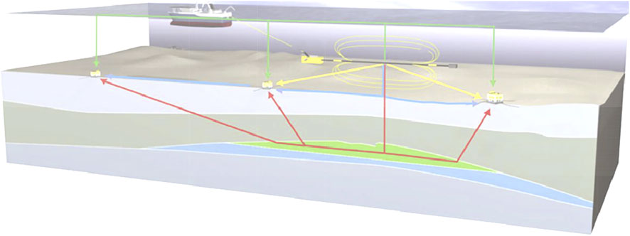
FIGURE 1. Configuration of the marine CSEM exploration system with deep near-seafloor towed horizontal electric dipole (HED) transmitter and multiple ocean bottom receiver array arrangements along the survey line. The two-dimensional survey grid is composed of multiple survey lines that can carry out 3D exploration The ship towed a long cable with the HED transmitter close to the seafloor to enhance the weak response signal from beneath the seafloor. The low-frequency electromagnetic wave with a controllable waveform is transmitted by the transmitter. The wave propagates to the surrounding areas, including 1) penetrating the submarine stratum and HC that was received by the receiver (red line), 2) propagation in seawater that was received by the receiver (yellow line), 3) propagation through the seafloor (blue line), 4) propagation through the sea surface (green line). If the receiver can measure the obvious electromagnetic response signal from HC, it can help us detect the distribution structure of HC.
The transmitting electrodes are placed at a certain height above the seafloor and excite a low-frequency electromagnetic wave signal which is simultaneously propagated through the seawater and the seafloor strata (Figure 1). Measuring points are placed on the surface of the seafloor to measure the electric or magnetic field. The electromagnetic waves received by the measuring device are direct, air, reflected, and refracted waves (Figure 1). The ship is towed with the transmitting dipole moving at a constant speed during the measurement. The frequency of excitation of the transmitting source is generally between 0.01 and 10 Hz, and in practice, the excitation occurs once every 50–200 m of towing. After the start of the measurement, the receiving system continuously receives and records the signals of the multiple electromagnetic components propagating from the seabed and seawater.
2.2 Modeling by the integral equation
To build a three-dimensional ocean model, it is assumed that the electrical conductivities of air, seawater, submarine sediment, and HC are
where
where
The electric field E in Eq. 4 contains both the incident and scattered fields, so
To solve for the scattered field
Based on the method of integral equations combined with the theory of dyadic Green’s function, the following integral equations are obtained by transforming and simplifying Eqs. 1 and 2:
where
With Eq. 7 in the case where the incident field (i.e., primary field)
The 3D target body is dissected into n small cells, while assuming that the electric field inside each dissected cell is constant and equal to the electric field at its center, then Eq. 3 can be written as follows:
Thus, the expression for the electric field at the center of the m-th cell is obtained as follows:
where
where
When the IP effect exists, the resistivity of rock and ore will change with frequency, that is, the complex resistivity spectrum. Using complex resistivity ρ (iω) instead of real resistivity ρ0, the electric field at the center of each cell can be obtained by solving matrix Eq. 10. Then, the response of the electric field at any point in space can be obtained using Eq. 7.
2.3 Induced polarization in controlled-source electromagnetic method
The IP phenomenon is usually associated with charging and discharging effects in the rock formation in the process of current injecting. Schlumberger (1920) discovered the phenomenon of induced polarization and used it in geophysical exploration. Subsequently, many geophysicists made contributions to the research methods (Sternberg, 1991; Zonge et al., 2005; Seigel et al., 2007; Veeken et al., 2009; Marchant et al., 2013; Tarasov and Titov, 2013; Ji et al., 2020). Chargeability is a physical property related to conductivity. As we learned previously, ionic charges within a rock’s pore water begin to move under the influence of an electric field, resulting in an electrical current. However, some of the pore ions do not move uninhibited through the rock and begin to accumulate at impermeable boundaries. This build-up of ionic charges is commonly referred to as induced polarization (IP), as it is responsible for generating electric dipole moments within the rock. Despite the complexity, there are two primary phenomenological mechanisms that are insightful in characterizing the chargeable behavior of rocks: membrane polarization and electrode polarization.
There are many factors affecting the charging rate, mainly in the following aspects: 1) clays; 2) pore water salinity; 3) sulfide mineralization; 4) tortuosity. Figure 2 schematically illustrates the typical IP effect from clays. Clays have a tendency to partially block the path which ions take through the rock’s pore water. Upon application of an electric potential, positive charge carriers pass easily, while negative carriers accumulate. This results in an “ion-selective” membrane polarization. Clays represent a dominant source of induced polarization in unmineralized sedimentary rocks.
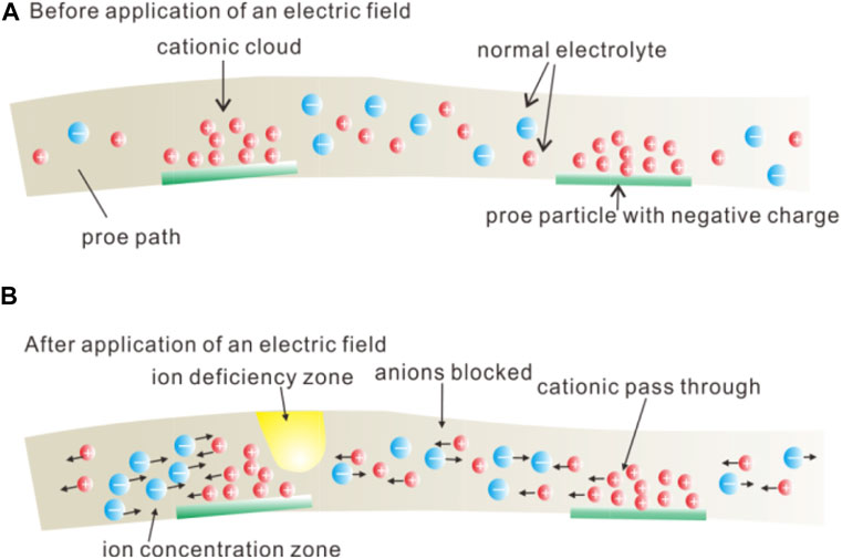
FIGURE 2. Schematic diagram of membrane polarization in rock containing clay particles and (A) rock with clay before the application of an electric field; (B) after the application of an electric field.
IP can be observed in time domain signals and frequency domain signals in electromagnetic exploration. The IP effect can be expressed as a percentage frequency effect (PFE) in the frequency domain, which is defined as the relative difference between apparent resistivity with a higher frequency
But this technique is noise-prone and susceptible to EM coupling effects. Thus, the IP effect in the frequency domain is usually measured by the phase shift, or time delay, between the transmitted current and the received voltage.
Figure 3 schematically illustrates the IP effects in the frequency domain. The waveform of the transmitted current and received voltage of CSEM with a transmitted fundamental frequency of 1 Hz. There is an obvious phase difference between the transmitting current and the receiving voltage, and the amplitude also decreases slightly.
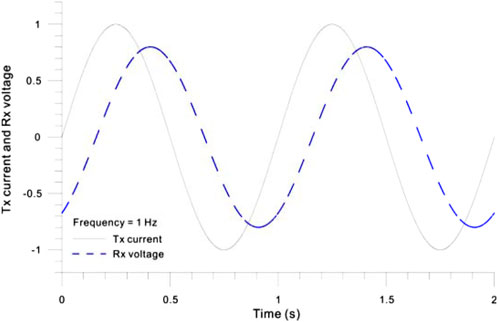
FIGURE 3. Representation of the IP effects in the frequency domain. The waveform of the transmitted current and received voltage of CSEM with a transmitted fundamental frequency of 1 Hz with the IP effects. There is an obvious phase difference between the transmitting current and the receiving voltage, and the amplitude also decreases slightly.
2.4 Complex resistivity with induced polarization
The parameters used to represent the IP effect of rock ores at small excitation currents can be considered linear time-invariant systems. Therefore, when the frequency of the emitted current varies, the corresponding received potential difference is the variable about frequency, ΔU (ω), and therefore the resistivity obtained from the transfer function R(ω) = U(ω)/I(ω) is also a function about frequency and is the complex resistivity. We usually use an equivalent circuit to describe the physical process of the IP effect in rocks and ores. However, this description has uncertainties, as the equivalent circuit model is different for different structures of rock ore. Sometimes, the same response can be obtained with different equivalent circuit models for the same rock ore, as its structure is microscopic in nature.
Although the induced polarization effect of rocks and minerals cannot be accurately described, it is still feasible to use some simplified equivalent models to approximate it (Titov et al., 2002; Zhdanov, 2008). When representing a polarized rock ore in an equivalent model, a basic unit can be approximated into four components: a conductive mineral component, a non-conductive mineral component, a pore filled with conductive minerals, and a pore filled with non-conductive minerals (as shown in Figure 2). The constituent parts of a rock ore that produce electrolysis include minerals with ion-exchange capacity and impregnated metals, which are linked by pores filled with ionic solutions.
This understanding of rock polarization is first due to the free movement between the ionic solution and solid conductive (metallic) or ion-exchange capable (clay, zeolite, and some other organic) particles in the vicinity of the contact surface. There are three commonly used ion polarization models to study the effect of electromagnetic induced polarization: the Cole–Cole model (Zhdanov, 2008), the Dias model (Merriam, 2007), and the short narrow pore (SNP) model (Titov et al., 2002). This article will study the influence of the IP parameters in the three models on the electric field response.
1) The Cole–Cole model. The following formula can be used (Zhdanov, 2008):
where ρ (ω) is the complex resistivity of the polarizable rock; ρ0 is the resistivity at zero frequency; m is the chargeability or polarizability; τ is the time constant; c is the frequency correlation coefficient.
2) The Dias model expression. The following formula can be used (Merriam, 2007):
where ρ (ω) is the rock complex resistivity at various frequencies, ρ0 is the resistivity at zero frequency, m is the polarizability, τ, τ′, and τ′′ represent various relaxation mechanisms,
3) The SNP model expression. The following formula can be used (Titov et al., 2002):
where ρ(ω) is the rock complex resistivity at various frequencies, ρ0 is the resistivity at frequency 0 Hz, m is the polarizability, and τ is the relaxation time.
3 Results
We studied the response law of different ion polarization models and analyzed the influence law of various model parameters. We have calculated the model from the following aspects: 1) the 1D/3D HC model in CSEM; 2) the influence of the Cole–Cole model on CSEM, including the effect of the polarizability, time constant, and frequency correlation coefficient; 3) the influence of the Dias model on CSEM, including the effect of the polarizability, time constant, frequency correlation coefficient, and volume percentage; 4) the influence of the SNP model on CSEM, including the effect of the polarizability, time constant, and frequency correlation coefficient.
3.1 1D and 3D hydrocarbons in controlled-source electromagnetic method
In order to verify the correctness and accuracy of the theory, our 3D calculation results were compared with those of the 1D model program of Kerry Key (2009). The emission current was set as I = 1 A, frequency: 0.1 Hz, dipole source length: 1 m, source height: 40 m from the seafloor, receiving point at the origin, seawater depth: 300 m, seawater resistivity: 0.3 Ωm, rock resistivity: 1 Ωm, HC resistivity: 100 Ωm, HC depth below seafloor: 1 km, and HC size: 50 × 50 × 0.1 km3.
Figure 4 shows the calculated magnitude of electric fields Ex in the geoelectric model with and without HC. The calculated Ex field of the 3D model is consistent with that using Key’s 1D program. For the model with the presence of HC, the offset distance is 1–3 km, and our 3D calculation is slightly lower than the 1D program. This is due to the fact that the finite length of the HC in the horizontal direction in the 3D model contributes slightly less to the Ex field value than the infinite length of the HC in the horizontal direction in the 1D model. Therefore, the 3D calculation results in this study are credible.
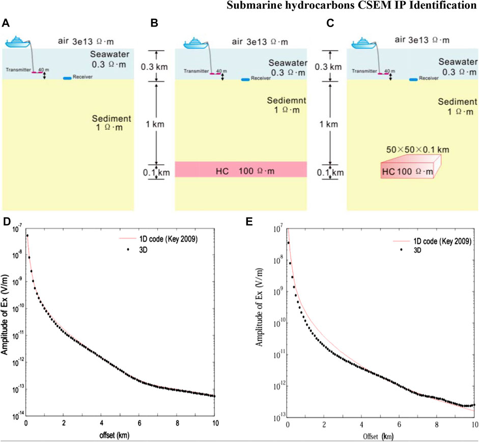
FIGURE 4. Geoelectric model of HC and corresponding forward calculation Ex versus offset in the 1D and the 3D marine CSEM. (A) 1D model with seafloor depth = 0.3 km; (B) 1D model with HC below seafloor = 1 km; (C) 3D model with HC below seafloor = 1 km and the size = 50 × 50 × 0.1 km3; (D) calculated magnitude of electric fields Ex versus offset (km) from the 1D and the 3D model without HC in (A,B);(E) calculated magnitude of electric fields Ex versus offset (km) from the 1D and the 3D model with HC in (C).
3.2 Induced polarization of the Cole–Cole model in a controlled-source electromagnetic method
We have compared the results of the Cole–Cole models of the HC with various parameters in the 3D CSEM.
3.2.1 Polarizability
We have compared the model responses of various polarizability coefficients to study the effect of the polarizability on CSEM with the IP using the Cole–Cole model. Use the following parameters: transmitted frequency f = 0.1 Hz, time constant τ = 1.0 s, frequency correlation coefficient c = 0.25, and polarizability m = 0.01, 0.05, 0.1, and 0.2. The height of the dipole source: 40 m. The receiver is at the origin. The origin of the coordinate is directly above the center point of the 3D HC. The seawater depth: 300 m, the seawater resistivity: 0.3 Ωm, the marine sediment resistivity: 1 Ωm, the resistivity of HC is 100 Ωm, the buried depth of HC: 1 km, and the size of HC: 5 × 2 × 0.1 km3.
Figure 5 shows the amplitude and phase ratio curves of the IP field to the pure electromagnetic field under different polarization rates of the Cole–Cole model, respectively. As can be seen from this result, within the offset distance of 1 km, the ratio of the IP field to the pure electromagnetic field is 1, indicating that the electromagnetic induction effect was dominant in this region, while the influence the IP effect was very weak; as the offset distance increases, the ratio is greater than 1; as the offset distance is in the range of 1–2 km, the ratio reaches the peak and then decreases to 1. In the interval, where the ratio is greater than 1, the polarization field is in the same direction as the electromagnetic field. The larger the m, the larger the polarization field, and the higher the total field amplitude.
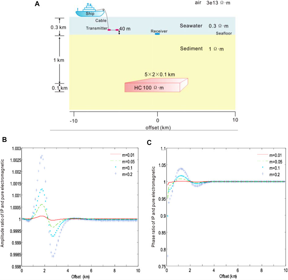
FIGURE 5. Amplitude and phase ratio of CSEM with the IP and pure electromagnetic field to the Cole–Cole model of various polarizability m = 0.01 (red), 0.05 (green), 0.1 (blue), and 0.2 (light blue), respectively. (A) Geoelectric model of submarine hydrocarbons with ion-induced polarization in the 3D marine CSEM, (B) the ratio of amplitude, and (C) the ratio of phase.
As the offset distance continues to increase, the ratio decreases from 1, and there is a minimum value near the boundary of the anomaly between 2 and 3 km, after which the ratio increases to 1 with the increase of the offset distance. In the interval, where the ratio is less than 1, the polarized field is in the opposite direction to the electromagnetic field, and the larger the m, the larger the polarized field, and the lower the total field amplitude.
When the offset distance is greater than 4 km, the ratio converges to 1, mainly dominated by the electromagnetic induction effect, and the IP effect can be ignored. From this figure, it can be seen that once the offset distance is greater than 1 km, the phase ratio curve of the IP field and the pure electromagnetic field is basically the same as the change of its amplitude curve.
3.2.2 Time constant
We have compared the model responses of various time constants to study the effect of the polarizability on CSEM with the IP using the Cole–Cole model. Use the following parameters: transmitted frequency f = 0.1 Hz, polarizability m = 0.1, and frequency correlation coefficient c = 0.25. Time constants τ = 1, 10, 100, and 1,000 s. The height of the dipole source: 40 m. The receiver is at the origin. The origin of the coordinate is directly above the center point of the 3D HC. The seawater depth: 300 m, the seawater resistivity: 0.3, the marine sediment resistivity: 1 Ωm, the resistivity of HC: 100 Ωm, the buried depth of HC: 1 km, and the size of HC: 5 × 2 × 0.1 km3.
Figure 6 shows the amplitude and phase ratio curves of the IP field to the pure electromagnetic field under different time constants of the Cole–Cole model, respectively. As can be seen from the result, within the offset distance of 1 km, the ratio of the IP field to the pure electromagnetic field is 1, indicating that the electromagnetic induction effect was dominant in this region while the influence of the IP effect was very weak; as the offset distance increases, the ratio is greater than 1; as the offset distance is in the range of 1–2 km, the ratio reaches the peak and then decreases to 1. In the interval, where the ratio is greater than 1, the polarization field is in the same direction as the electromagnetic field, and the larger the τ, the smaller the polarization field, and the lower the total field amplitude.
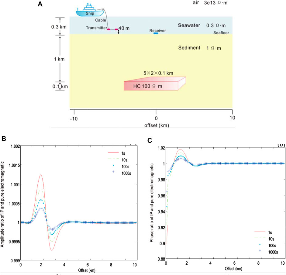
FIGURE 6. Amplitude and phase ratio of CSEM with the IP and pure electromagnetic field to the Cole–Cole model of various time constants τ = 1 (red), 10 (green), 100 (blue), and 1,000 (light blue), respectively. (A) Geoelectric model of submarine hydrocarbons with ion-induced polarization in the 3D marine CSEM, (B) the ratio of amplitude, and (C) the ratio of phase.
As the offset distance continues to increase, the ratio decreases from 1, and there is a minimum value near the boundary of the anomaly between 2 and 3 km, after which the ratio increases to 1 with the increase of the offset distance. In the interval, where the ratio is less than 1, the polarized field is in the opposite direction to the electromagnetic field, and the larger the τ, the smaller the polarized field and the higher the total field amplitude. When the offset distance is greater than 4 km, the ratio converges to 1, mainly dominated by the electromagnetic induction effect, and the IP effect can be ignored. From this result, it can be seen that once the offset distance is greater than 1 km, the phase ratio curve of the IP field and the pure electromagnetic field is basically the same as the change of its amplitude curve.
3.2.3 Frequency correlation coefficient
We have compared the model responses of various frequency correlation coefficients to study the effect of this coefficient on CSEM with the IP using the Cole–Cole model. Use the following parameters: transmitted frequency f = 0.1 Hz, polarizability m = 0.1, time constant τ = 1.0 s, and frequency correlation coefficient c = 0.2, 0.4, 0.6, and 0.8. The height of the dipole source: 40 m. The receiver is at the origin. The origin of the coordinate is directly above the center point of the 3D HC. The seawater depth: 300 m, the seawater resistivity: 0.3 Ωm, the marine sediment resistivity: 1 Ωm, the resistivity of HC: 100 Ωm, the buried depth of HC: 1 km, the size of HC: 5 × 2 × 0.1 km3.
Figure 7 shows the amplitude and phase ratio curves of the IP electric field to the pure electromagnetic field under different frequency correlation coefficients of the Cole–Cole model, respectively. As can be seen from this result, within an offset of 1 km, the ratio of the IP electric field to the pure electromagnetic field was 1, indicating that within this interval, the electromagnetic induction effect was dominant while the influence of the IP effect was very weak. With the increase in offset, there was a maximum value between 1 and 2 km. Between 1 and the maximum value on the curve, the polarization field decreased with the increase of the frequency correlation coefficient c.
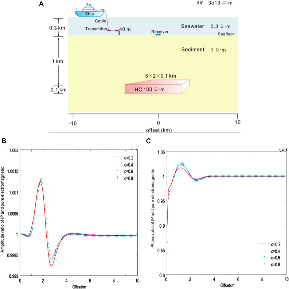
FIGURE 7. Amplitude and phase ratio of CSEM with the IP and pure electromagnetic field to the Cole–Cole model of various frequency correlation coefficients c = 0.2 (red), 0.4 (green), 0.6 (blue), and 0.8 (light blue), respectively. (A) Geoelectric model of submarine hydrocarbons with ion-induced polarization in the 3D marine CSEM, (B) the ratio of amplitude, and (C) the ratio of phase.
As the offset continued to increase until the ratio decreased to 1, within the interval from the maximum value to the ratio of 1, the polarization field increased with c. There was a minimum value between 2 and 3 km, which then increased to 1–4 km. In this interval, with the increase of c, the polarization field decreased. When the offset was greater than 4 km, the ratio tended to be 1 due to the electromagnetic induction effect, and the influence of the IP effect was weak. According to this result, the phase ratio was less than 1 within 1 km of the offset. When the offset was greater than 1 km, generally, the phase ratio curve of the IP electric field to the pure electromagnetic field was consistent with that of the amplitude curve of the IP electric field to the pure electromagnetic field.
3.3 Induced polarization of the Dias model in a controlled-source electromagnetic method
We have compared the results of the Cole–Cole models of the Dias with various parameters in 3D CSEM.
3.3.1 Polarizability
We have compared the model responses of various polarizability coefficients to study the effect of the polarizability on CSEM with the IP using the Dias model. Use the following parameters: transmitted frequency f = 0.1 Hz, time constant τ = 1.0 s, electrochemical parameter η = 10 s−1/2, volume percentage δ = 0.2, and polarizability m = 0.01, 0.05, 0.1, and 0.2. The height of the dipole source: 40 m. The receiver is at the origin. The origin of the coordinate is directly above the center point of the 3D HC. The seawater depth: 300 m, the seawater resistivity: 0.3 Ωm, the marine sediment resistivity: 1 Ωm, the resistivity of HC: 100 Ωm, the buried depth of HC: 1 km, and the size of HC: 5 × 2 × 0.1 km3.
Figure 8 shows the amplitude and phase ratio curves of the IP electric field to the pure electromagnetic field under different polarizabilities of the Dias model, respectively. As can be seen from Fig. 5.8, within the 1 km offset, the ratio of the IP electric field to the pure electromagnetic field was 1, indicating that the electromagnetic induction effect was dominant while the influence of the IP effect was very weak. Between 1 and 2 km, the ratio was greater than 1, and there was a maximum value. Within this interval, the polarization field was consistent with the electromagnetic field in direction. The larger the m value, the larger the polarization field, and the higher the total field amplitude. Within 2–4 km, there was a minimum value, and the point for the minimum value was just located 2.5 km near the boundary of the HC body. Within the interval, the ratio was less than 1, and the direction of the polarization field was opposite to that of the electromagnetic field. The larger the m value, the larger the polarization field, and the lower the total field amplitude.
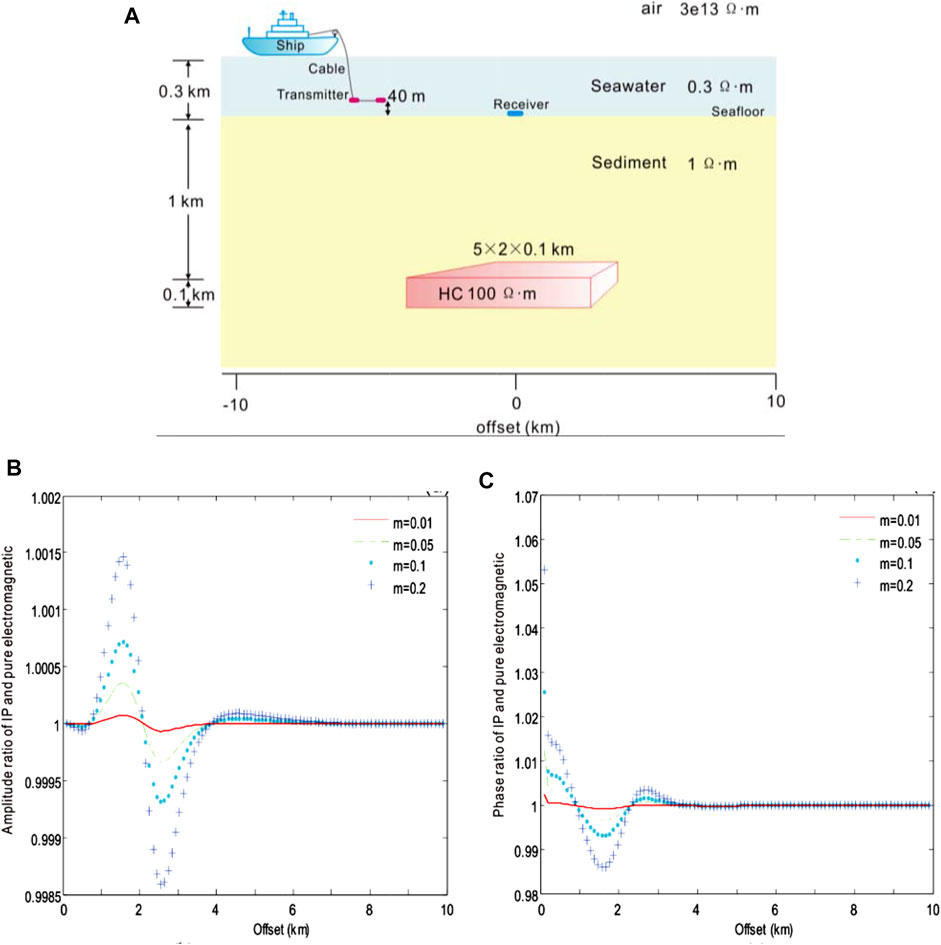
FIGURE 8. Amplitude and phase ratio of CSEM with the IP and pure electromagnetic field to the Dias model of various polarizability m = 0.01 (red), 0.05 (green), 0.1 (blue), and 0.2 (light blue), respectively. (A) Geoelectric model of submarine hydrocarbons with ion-induced polarization in the 3D marine CSEM, (B) the ratio of amplitude, and (C) the ratio of phase.
When the offset was greater than 4 km, the ratio tended to be 1 due to the electromagnetic induction effect, and the influence of the IP effect was weak. According to this result, within 1–4 km, the phase ratio curve of the IP electric field to the pure electromagnetic field was opposite to that of the amplitude curve of the IP electric field to the pure electromagnetic field generally. When the offset was greater than 4 km, the ratio tended to be 1, and the effect of IP was weak.
3.3.2 Time constant
We have compared the model responses of various time constants to study the effect of the time constant on CSEM with the IP using the Dias model. Use the following parameters: transmitted frequency f = 0.1 Hz, polarizability m = 0.1, electrochemical parameter η = 10 s−1/2, volume percentage δ = 0.2, and Time constants τ = 1, 10, 100 and 1,000 s. The height of the dipole source: 40 m. The receiver is at the origin. The origin of the coordinate is directly above the center point of the 3D HC. The seawater depth: 300 m, the seawater resistivity: 0.3 Ωm, the marine sediment resistivity: 1 Ωm, the resistivity of HC: 100 Ωm, the buried depth of HC: 1 km, and the size of HC: 5 × 2 × 0.1 km3.
Figure 9 shows the amplitude and phase ratio curves of the IP electric field to the pure electromagnetic field under different time constants of the Dias model respectively. According to this result, within the 1 km offset, the ratio of the IP electric field to the pure electromagnetic field was approximately 1, indicating that the electromagnetic induction effect was dominant while the influence of the IP effect was very weak. Within 1–2 km, the ratio was greater than 1, and there was a maximum value. Within this interval, the polarization field was consistent with the electromagnetic field in direction. The larger the τ value, the smaller the polarization field, and the lower the total field amplitude. Within 2–4 km, there was a minimum value, and the point for the minimum value was just located 2,500 m near the boundary of the HC body. Furthermore, in this interval, the ratio was less than 1, and the direction of the polarization field was opposite to that of the electromagnetic field. The larger the τ value, the smaller the polarization field, and the higher the total field amplitude.
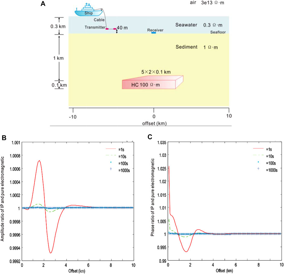
FIGURE 9. Amplitude and phase ratio of CSEM with the IP and pure electromagnetic field to the Dias model of various time constants τ = 1 (red), 10 (green), 100 (blue), and 1,000 (light blue), respectively. (A) Geoelectric model of submarine hydrocarbons with ion-induced polarization in the 3D marine CSEM, (B) the ratio of amplitude, and (C) the ratio of phase.
When the offset was greater than 4 km, the ratio tended to be 1 due to the electromagnetic induction effect, and the influence of the IP effect was weak. According to this result, within 1–4 km, the phase ratio curve of the IP electric field to the pure electromagnetic field was opposite to that of the amplitude curve of the IP electric field to the pure electromagnetic field generally. When the offset was greater than 4 km, the ratio tended to be 1, and the effect of IP was weak.
3.3.3 Electrochemical parameter
We have compared the model responses of various electrochemical parameters to study the effect of the electrochemical parameter on CSEM with the IP using the Dias model. Use the following parameters: transmitted frequency f = 0.1 Hz, polarizability m = 0.1, time constants τ = 1.0 and 0.2 s, and electrochemical parameters η=5 s−1/2, 10 s−1/2, 50 s−1/2, and 100 s−1/2, respectively. The height of the dipole source: 40 m. The receiver is at the origin. The origin of the coordinate is directly above the center point of the 3D HC. The seawater depth: 300 m, the seawater resistivity: 0.3 Ωm, the marine sediment resistivity: 1 Ωm, the resistivity of HC: 100 Ωm, the buried depth of HC: 1 km, and the size of HC: 5 × 2 × 0.1 km3.
Figure 10 shows the amplitude and phase ratio curves of the IP electric field to the pure electromagnetic field under different electrochemical parameters of the Dias model, respectively. According to this result, within the 1 km offset, the ratio of the IP electric field to the pure electromagnetic field was 1, indicating that the electromagnetic induction effect was dominant while the influence of the IP effect was very weak. Within 1–2 km, the ratio was greater than 1, and there was a maximum value. Within this interval, the polarization field was consistent with the electromagnetic field in direction. The larger the η value, the larger the polarization field, and the higher the total field amplitude. Between 2 and 4 km, there was a minimum value, and the point for the minimum value was just located 2.5 km near the boundary of the HC body. Within this interval, the ratio was less than 1, and the direction of the polarization field was opposite to that of the electromagnetic field. The larger the η value, the larger the polarization field, and the lower the total field amplitude.
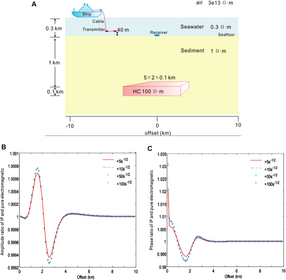
FIGURE 10. Amplitude and phase ratio of CSEM with the IP and pure electromagnetic field to the Dias model of various electrochemical parameters η = 5 s−1/2 (red), 10 s−1/2 (green), 50 s−1/2 (blue), and 100 s−1/2 (light blue), respectively. (A) Geoelectric model of submarine hydrocarbons with ion-induced polarization in the 3D marine CSEM, (B) the ratio of amplitude, and (C) the ratio of phase.
When the offset was greater than 4 km, the ratio tended to be 1 due to the electromagnetic induction effect, and the influence of the IP effect was weak. According to this result, between 1 and 4 km, the phase ratio curve of the IP electric field to the pure electromagnetic field was opposite to that of the amplitude curve of the IP electric field to the pure electromagnetic field generally. When the offset was greater than 4 km, the ratio tended to be 1.
3.3.4 Volume percentage
We have compared the model responses of various volume percentages to study the effect of volume percentage on CSEM with the IP using the Dias model. Use the following parameters: transmitted frequency f = 0.1 Hz, polarizability m = 0.1, time constant τ = 1.0 s, electrochemical parameter η = 10 s−1/2, and volume percentage δ = 0.2, 0.4, 0.6, and 0.8. The high of the dipole source: 40 m. The receiver is at the origin. The origin of the coordinate is directly above the center point of the 3D HC. The seawater depth: 300 m, the seawater resistivity: 0.3 Ωm, the marine sediment resistivity: 1 Ωm, the resistivity of HC: 100 Ωm, the buried depth of HC: 1 km, and the size of HC: 5 × 2 × 0.1 km3.
Figure 11 shows the amplitude and phase ratio curves of the IP electric field to the pure electromagnetic field under different volume percentages of the Dias model, respectively. According to this result, within the 1 km offset, the ratio of the IP electric field to the pure electromagnetic field was 1, indicating that the electromagnetic induction effect was dominant while the influence of the IP effect was very weak. Within 1–2 km, the ratio was greater than 1, and there was a maximum value. In this interval, the polarization field was consistent with the electromagnetic field in direction. The larger the δ value, the larger the polarization field, and the higher the total field amplitude. Between 2 and 4 km, there was a minimum value, and the point for the minimum value was just located 2.5 km near the boundary of the HC body. Within the interval, the ratio was less than 1, and the direction of the polarization field was opposite to that of the electromagnetic field. The larger the δ value, the larger the polarization field, and the lower the total field amplitude.
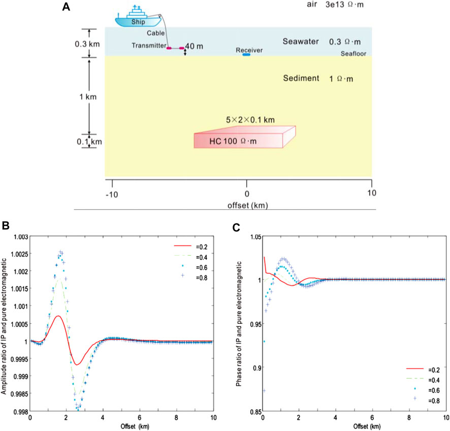
FIGURE 11. Amplitude and phase ratio of CSEM with the IP and pure electromagnetic field to the Dias model of various volume percentages δ = 0.2 (red), 0.4 (green), 0.6 (blue) and 0.8 (light blue), respectively. (A) Geoelectric model of submarine hydrocarbons with ion-induced polarization in the 3D marine CSEM, (B) the ratio of amplitude, and (C) the ratio of phase.
When the offset was greater than 4 km, the ratio tended to be 1 due to the electromagnetic induction effect, and the influence of the IP effect was weak. According to this result, between 1 and 4 km, the phase ratio curve of IP electric field to the pure electromagnetic field was opposite to the amplitude curve of IP electric field to the pure electromagnetic field generally. When the offset was greater than 4 km, the ratio tended to be 1.
3.4 Induced polarization of the short narrow pore model in a controlled-source electromagnetic method
We have compared the results of the SNP models of the Dias with various parameters in 3D CSEM.
3.4.1 Polarizability
We have compared the model responses of various polarizability coefficients to study the effect of the polarizability on CSEM with the IP using the SNP model. Use the following parameters: transmitted frequency f = 0.1 Hz, time constant τ = 1.0 s, and polarizability m = 0.01, 0.05, 0.1, and 0.2. The height of the dipole source: 40 m. The receiver is at the origin. The origin of the coordinate is directly above the center point of the 3D HC. The seawater depth: 300 m, the seawater resistivity: 0.3 Ωm, the marine sediment resistivity: 1 Ωm, the resistivity of HC: 100 Ωm, the buried depth of HC: 1 km, and the size of HC: 5 × 2 × 0.1 km3.
Figure 12 shows the amplitude and phase ratio curves of the IP electric field to the pure electromagnetic field under different polarizabilities of the SNP model. According to this result, within the 1 km offset, the ratio of the IP electric field to the pure electromagnetic field was 1, indicating that the electromagnetic induction effect was dominant while the influence of the IP effect was very weak. Between 1 and 2 km, the ratio was greater than 1, and there was a maximum value. In this interval, the polarization field was consistent with the electromagnetic field in direction. The larger the m value, the larger the polarization field, and the higher the total field amplitude. Within 2–4 km, there was a minimum value, and the point for the minimum value was just located 2.5 km near the boundary of the HC body. Within the interval, the ratio was less than 1, and the direction of the polarization field was opposite to that of the electromagnetic field. The larger the m value, the larger the polarization field, and the lower the total field amplitude.
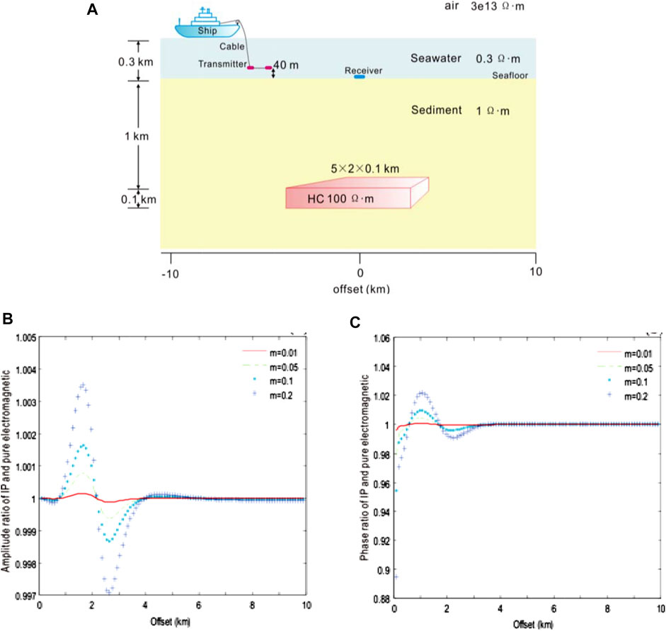
FIGURE 12. Amplitude and phase ratio of CSEM with the IP and pure electromagnetic field to the SNP model of various polarizability m = 0.01 (red), 0.05 (green), 0.1 (blue), and 0.2 (light blue), respectively. (A) Geoelectric model of submarine hydrocarbons with ion-induced polarization in the 3D marine CSEM, (B) the ratio of amplitude, and (C) the ratio of phase.
When the offset was greater than 4 km, the ratio tended to be 1 due to the electromagnetic induction effect, and the influence of the IP effect was weak. According to this result, between 1 and 4 km, the phase ratio curve of the IP electric field to the pure electromagnetic field was consistent with that of the amplitude curve of the IP electric field to the pure electromagnetic field generally.
3.4.2 Time constant
We have compared the model responses of various time constants to study the effect of the time constant on CSEM with the IP using the SNP model. Use the following parameters: transmitted frequency f = 0.1 Hz, polarizability m = 0.1, and time constants τ = 1, 10, 100, and 1,000 s. The height of the dipole source: 40 m. The receiver is at the origin. The origin of the coordinate is directly above the center point of the 3D HC. The seawater depth: 300 m, the seawater resistivity: 0.3 Ωm, the marine sediment resistivity: 1 Ωm, the resistivity of HC: 100 Ωm, the buried depth of HC: 1 km, and the size of HC: 5 × 2 × 0.1 km3.
Figure 13 shows the amplitude and phase ratio curves of the IP electric field to the pure electromagnetic field under different time constants of the SNP model, respectively. According to this result, within the 1 km offset, the ratio of the IP electric field to the pure electromagnetic field was 1, indicating that the electromagnetic induction effect was dominant while the influence of the IP effect was very weak. Within 1–2 km, the ratio was greater than 1, and there was a maximum value. In this interval, the polarization field was consistent with the electromagnetic field in direction. The larger the τ value, the smaller the polarization field, and the lower the total field amplitude. Within 2–4 km, there was a minimum value, and the point for the minimum value was just located 2.5 km near the boundary of the HC body. Within the interval, the ratio was less than 1, and the direction of the polarization field was opposite to that of the electromagnetic field. The larger the τ value, the smaller the polarization field, and the higher the total field amplitude. When the offset was greater than 4 km, the ratio tended to be 1 due to the electromagnetic induction effect, and the influence of the IP effect was weak. This result showed no obvious trend for the phase ratio curve of the IP electric field to the pure electromagnetic field.
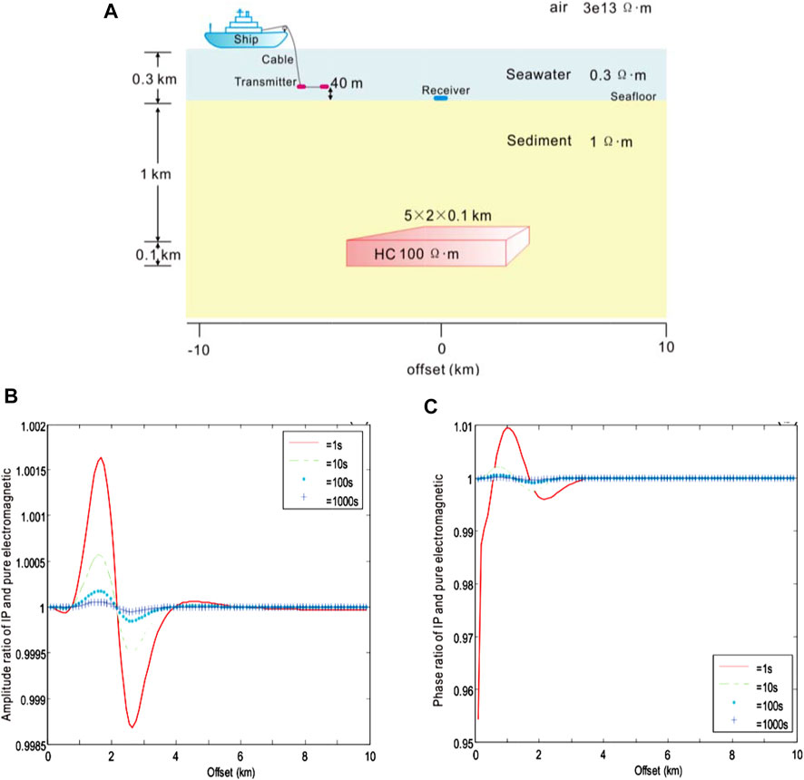
FIGURE 13. Amplitude and phase ratio of CSEM with the IP and pure electromagnetic field to the SNP model of various time constants τ = 1 (red), 10 (green), 100 (blue), and 1,000 (light blue), respectively. (A) Geoelectric model of submarine hydrocarbons with ion-induced polarization in the 3D marine CSEM, (B) the ratio of amplitude, and (C) the ratio of phase.
3.5 Field data
We used the marine CSEM data collected in the north of the South China Sea in 2019, in which the dipole distance is 200 m, the emission waveform is a square wave, the current is 950 A, and the emission frequency is 0.1 and 1 Hz. The inversion calculation fits the field amplitude and phase as shown in Figures 14 and 15 using frequencies 0.1 and 1 Hz. The figures show the field data and the inversion response with the Cole–Cole model of various polarizability m = 0 (pure electromagnetic field), 0.1, 0.3, 0.5, and 0.8. The inversion with the polarizability m = 0.5 is in the best agreement with the field data.
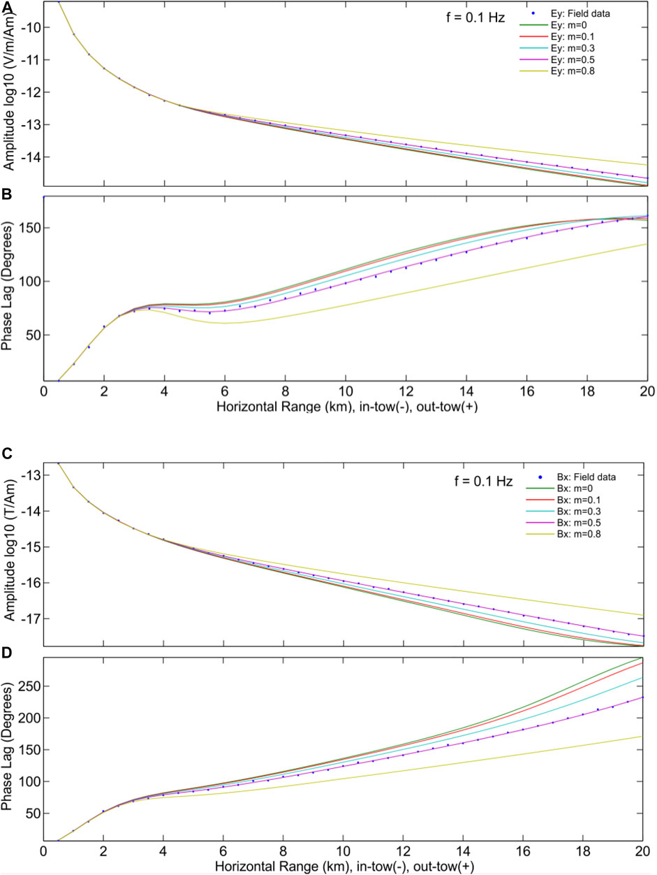
FIGURE 14. Log10 amplitude and phase (degrees) of f = 0.1 Hz CSEM field data [Ey (A,B) and Bx (C,D)]. Field data (blue) and inversion response with the Cole–Cole model of various polarizability m = 0 (pure electromagnetic field) (green), 0.1 (red), 0.3 (light blue), 0.5 (purple), and 0.8 (yellow), respectively.
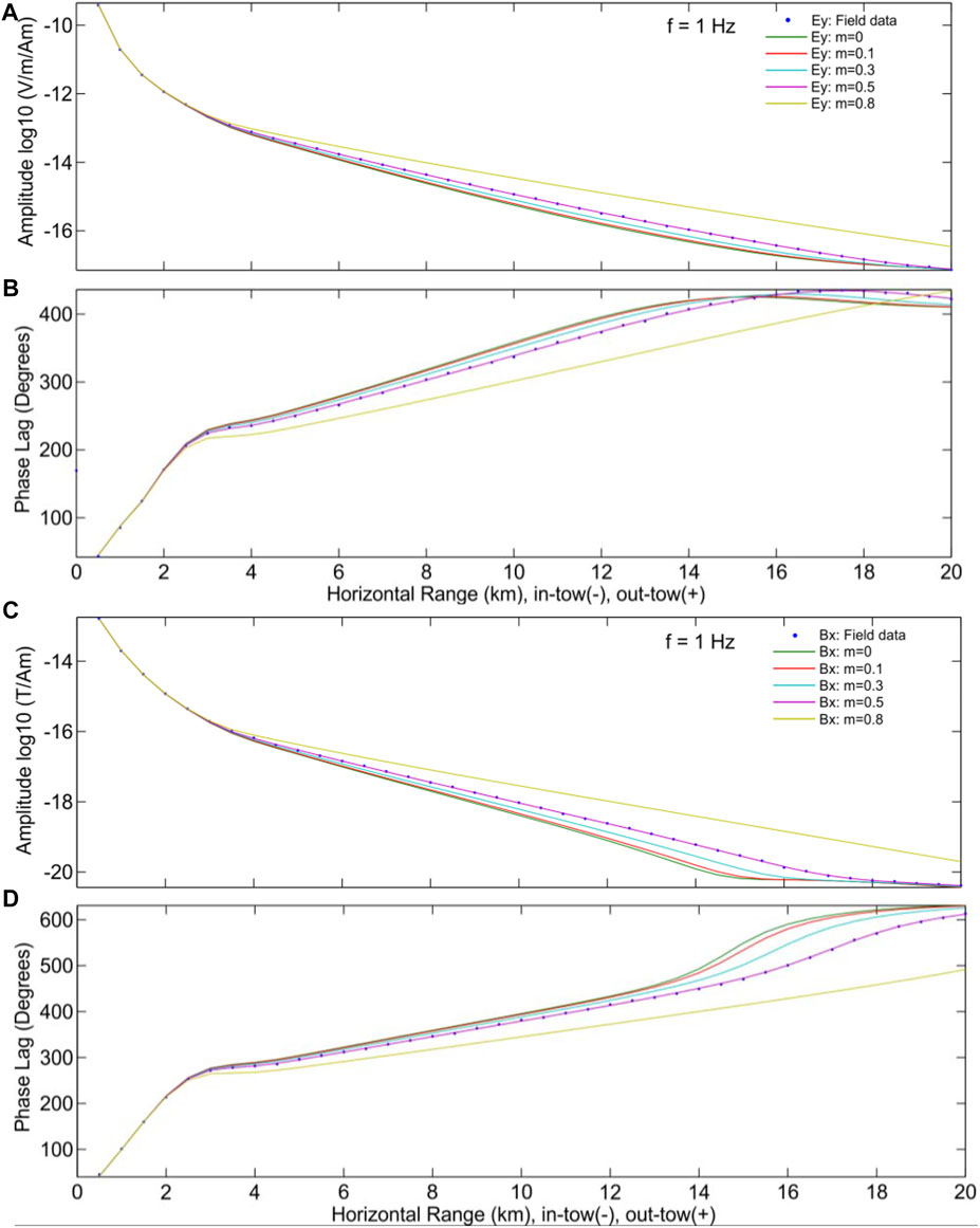
FIGURE 15. Log10 amplitude and phase (degrees) of f = 1 Hz CSEM field data [Ey (A,B) and Bx (C,D)]. Field data (blue) and inversion response with the Cole–Cole model of various polarizability m = 0 (pure electromagnetic field) (green), 0.1 (red), 0.3 (light blue), 0.5 (purple), and 0.8 (yellow), respectively.
The amplitude and phase response results of various polarizability show that the difference gradually increases from the offset to 2 km. It is revealed here that the IP effect begins to have a significant impact on the inversion results beyond the offset of 2 km.
By comparing the inversion responses of various frequencies, it can be seen that the IP response has an impact on both high-frequency and low-frequency data. The high-frequency signal itself attenuates rapidly with the increase of offset distance, but the larger polarizability contributes more to the data. At the same time, the response with larger polarizability will increase the data amplitude compared with that without IP polarizability.
For the low-frequency (0.1 Hz) emission signals of the marine CSEM, the amplitudes of the electric field with various polarization decrease with the offset increase (Figure 14A). When the offset is lower than 2.5 km, The electric field amplitude almost coincides and rapidly decreases by three orders of magnitude (∼10−12 V/m/Am). The attenuation of the amplitude decreases as the offset increases. When the offset is close to 20 km, the attenuation rate of the electric field amplitude approaches 0. The electric field with a larger polarizability has a relatively large amplitude for the same offset. For example, when the polarizability is 0.8, the amplitude is higher than that of 0.1 polarizability. In particular, when the offset is about 20 km, the difference between them is about an order of magnitude.
For the low-frequency (0.1 Hz) emission signals of the marine CSEM, the phase of the electric field with various polarization all increases with the offset (Figure 14B). When the offset is lower than 2.5 km, The electric field phase almost coincides and rapidly increases to about 70. The electric field with a larger polarizability has a relatively small change in phase for the same offset. For example, When the offset is about 12 km, the phase curve with the polarizability m = 0.8 is lower than the phase curve with other polarizabilities. In addition, when the offset is about 20 km, most phase curves tend to be about 150, except for the trends of the polarizability m = 0.8.
For the low-frequency (0.1 Hz) emission signals of the marine CSEM, the magnetic field's amplitudes with various polarization decrease with the offset (Figure 14C). When the offset is lower than 2.5 km, the electric field amplitude almost coincides and rapidly decreases by three orders of magnitude (∼10−16 V/m/Am). The attenuation of the amplitude decreases as the offset increases. When the offset is close to 20 km, the attenuation of magnetic field amplitude approaches 0. The magnetic field with a larger polarizability has a relatively large amplitude for the same offset. When the polarizability is 0.8, the amplitude is higher than that when the polarizability is 0.1. In particular, when the offset is 20 km, the difference between them is about an order of magnitude. The phase of most curves tends to be about 10−20 T/Am, except for the magnetic field with the polarizability m = 0.8.
For the low-frequency (0.1 Hz) emission signals of the marine CSEM, the magnetic field phase with various polarization increases with the offset (Figure 14D). When the offset is lower than 2.5 km, The magnetic field phase almost coincides and rapidly increases to about 230. The increase rate of phase gradually decreases with the increase of the offset. The magnetic field with a larger polarizability has a relatively small change in phase for the same offset. For example, When the offset is about 12 km, the phase curve with the polarizability m = 0.8 is obviously lower than the phase curve with other polarizabilities. In addition, when the offset is about 20 km, most phase curves tend to be about 150, except for the trends of the polarizability m = 0.8.
For the high-frequency (1 Hz) emission signals of the marine CSEM, the amplitudes of the electric field with various polarization decreases with the offset increase (Figure 15A). When the offset is lower than 2.5 km, the electric field amplitude almost coincides and rapidly decreases by three orders of magnitude (∼10−13 V/m/Am). The attenuation of the amplitude decreases as the offset increases. When the offset is close to 20 km, the attenuation rate of the electric field amplitude approaches 0. The electric field with a larger polarizability has a relatively large amplitude for the same offset. For example, when the polarizability is 0.8, the amplitude is higher than that when the polarizability is 0.1.In particular, when the offset is 20 km, the difference between them is about an order of magnitude.
For the high-frequency (1 Hz) emission signals of the marine CSEM, the phase of the electric field with different polarizabilities all increases with the increase of the offset (Figure 15B). When the offset is less than 2.5 km, the electric field phase almost coincides and rapidly increases to about 220. However, when the offset is above 2.5 km, the growth rate of the phase gradually decreases with the increase of offset. The electric field with a larger polarizability has a relatively small change in phase for the same offset. For example, When the offset is about 12 km, the phase curve with the polarizability being 0.8 is obviously lower than the phase curve with other polarizabilities. In addition, when the offset is about 20 km, most phase curves tend to be about 420, except for the trends of the polarizability being 0.8.
For the high-frequency (1 Hz) emission signals of the marine CSEM, the magnetic field amplitudes with various polarizabilities decreases with the offset (Figure 15C). When the offset is less than 2.5 km, the magnetic field amplitude almost coincides and rapidly decreases by three orders of magnitude (∼10−16 T/Am). The attenuation of the amplitude decreases as the offset increases. When the offset is close to 20 km, the attenuation rate of the electric field amplitude tends to be 0. The magnetic field with a larger polarizability has a relatively significant change in amplitude for the same offset. For example, when the polarizability is 0.8, the amplitude is higher than that when the polarizability is 0.1. In particular, when the offset is 20 km, the difference between them is about an order of magnitude. In particular, when the offset is 20 km, the difference between them is about an order of magnitude. The phase of most curves tends to be the minimum (∼10−20 T/Am), except for the magnetic field with the polarizability m = 0.8.
For the high-frequency (1 Hz) emission signals of the marine CSEM, the magnetic field phase with various polarizabilities increases with the offset (Figure 15C). When the offset is lower than 2.5 km, The magnetic field phase almost coincides and rapidly increases to about 280. However, when the offset is more than 2.5 km, the growth rate of the phase gradually decreases with the increase of offset. The magnetic field with a larger polarizability has a relatively small change in phase for the same offset. For example, When the offset is about 12 km, the phase curve with the polarizability m = 0.8 is obviously lower than the phase curve with other polarizabilities. In addition, the trends of most phase of most phase curves is about 620, except for the trends of polarizability of 0.8.
Figure 16 shows the resistivity inversion with various polarizability m = 0 (pure electromagnetic field), 0.1, 0.3, 0.5, and 0.8. The inversion result with polarizability is more consistent with the variation trends of seabed formation resistivity.
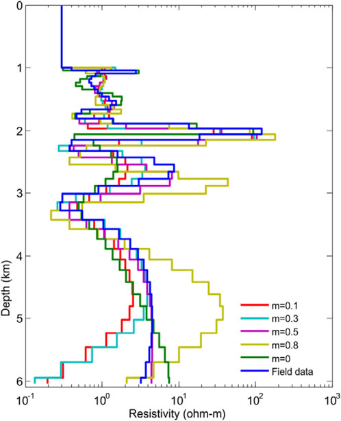
FIGURE 16. Inversion of resistivity from CSEM field data (blue) with various polarizability m = 0 (pure electromagnetic field) (green), 0.1 (red), 0.3 (light blue), 0.5 (purple), and 0.8 (yellow), respectively.
4 Discussion
4.1 Induced polarization of the Cole–Cole model
When considering HC for the IP response of the Cole–Cole model in CSEM, we identified the influence of Cole–Cole model parameters as follows: the larger the polarization field, the stronger the IP effect. The larger the time constant, the smaller the polarization field, and the weaker the IP effect. The influence of the frequency correlation coefficient was relatively complicated. Within an interval in the same direction as the pure electromagnetic field, with the increase of c, the polarization field first decreased and then increased, while in an interval opposite to the pure electromagnetic field in direction, with the increase of c, the polarization field decreased. The effects of polarization rate and time constant on the polarization field were more obvious and regular. So, they may be selected as parameters for inversion in data processing.
4.2 Induced polarization of the Dias model
When considering HC for the IP response of the Dias model in CSEM, we identified the influence of Dias model parameters as follows: the larger the polarizability, the larger the polarization field, and the stronger the IP effect. The larger the time constant, the smaller the polarization field, and the weaker the IP effect. The larger the electrochemical parameter, the larger the polarization field, and the stronger the IP effect. The larger the volume percentage, the larger the polarization field, and the stronger the IP effect. The parameters that affected the polarization field most significantly were the polarizability and volume percentage, followed by time constant and electrochemical parameters.
4.3 Induced polarization of the short narrow pore model
When considering HC for the IP response of the SNP model in CSEM, we identified the influence of the SNP model parameters as follows: the larger the polarizability, the larger the polarization field, and the stronger the IP effect. The larger the time constant, the smaller the polarization field, and the weaker the IP effect. Both polarization and time constant had a significant effect.
4.4 Influence of various polarizations on EM with offset and frequency
1) The amplitude and phase trends of the CSEM electromagnetic fields with various polarizabilities almost coincide at a small offset (<2.5 km) (Figures 14,15). It may be that CSEM signals observed from shallow layers are mainly direct wave signals propagating along the interface between seawater and seafloor. Without polarizability, these signals may not show polarization characteristics when passing through shallow media. Therefore, observing obvious polarization characteristics at a small offset (<2.5 km) is not easy.
2) At medium offset (3–20 km), the transmitter mainly receives the reflected signals of CSEM signals passing through oil and gas reservoirs, while the transmission of electromagnetic waves in hydrocarbon media will be different due to different polarizability reservoirs. Therefore, the phase curve has changed, showing the polarization characteristics. The greater the polarizability, the smaller the phase value, and the greater the polarizability, the greater the amplitude.
3) When the offset is large (>20 km), the phase difference and amplitude tend to be consistent because when the offset is too large, the received CSEM signal is dominated by airwaves, and the parameters of airwaves are consistent, so the polarization characteristics disappear at large offset (>20 km).
4) The difference between Figures 14,15 is that the maximum value of the phase difference and the minimum value of the amplitude of the received CSEM signal display different features. When the frequency increases, the propagation speed of the electrical signal remains unchanged, and the reservoir's propagation time remains unchanged at the same polarizability. According to the relationship between phase and frequency (ω=2πf), the greater the frequency, the greater the phase changes at the same time. According to the law of electromagnetic wave energy attenuation, the wavelength of the electromagnetic wave is inversely proportional to the frequency. The higher the frequency is, the shorter the wavelength is. The transmission of the electromagnetic wave is easier to be blocked by small objects, so the amplitude of the electromagnetic wave attenuates faster.
5 Conclusion
In this study, the influence of multiple ion polarization models on the IP effect in marine controlled-source electromagnetic method for offshore oil and gas was evaluated by integral equation forward modeling, the scattering and stacking methods were used to calculate the dyadic Green’s function needed in the study, and the real resistivity was replaced with the complex resistivity considering the IP effect to obtain the 3D marine CSEM forward algorithm incorporating the IP effect.
The influence of parameters in various ion polarization models has been analyzed, and the conclusion is as follows: through calculating the responses of three common ion polarization models, we have found that within a small offset range, the polarization field is first consistent with and then opposite to the pure electromagnetic field in direction. In the same direction, the total field amplitude is strengthened; otherwise, the total field amplitude is weakened. Limited by three-dimensional scale, at a large offset, the electromagnetic induction effect is dominant while the influence of the IP effect is weak.
The polarization rate and time constant of the Cole–Cole model have more obvious and regular effects on the polarization field, and so they may be selected as parameters for inversion in data processing. The parameters that may affect the polarization field most significantly are the polarizability and volume percentage, followed by time constant and electrochemical parameters. For the SNP model, both polarization and time constant have a significant effect.
The field data also show the amplitude and phase response results of polarizability show that it gradually increases from the offset. The IP response has an impact on both high-frequency and low-frequency data. The larger polarizability may increase the amplitude.
Data availability statement
The original contributions presented in the study are included in the article/Supplementary Material; further inquiries can be directed to the corresponding authors.
Author contributions
NQ: conceptualization, data interpretation, writing, and funding acquisition. QF: data interpretation and writing. YC: supervision and data interpretation. BD: writing and funding acquisition.
Funding
This study was funded by the Key Special Project for Introduced Talents Team of Southern Marine Science and Engineering Guangdong Laboratory (GML2019ZD0104, 2019BT02H594), Guangdong Basic and Applied Basic Research Foundation (Natural Science Foundation of Guangdong Province) (2021A1515011526, 2020B1111520001), Hainan Key Laboratory of Marine Geological Resources and Environment (HNHYDZZYHJKF010), NSFC(U2244221), Guangdong Provincial Research and Development Program in key areas (2020B1111520001), the Key Laboratory of Geophysical Electromagnetic Probing Technologies of Ministry of Natural Resources (KLGEPT202001).
Conflict of interest
The authors declare that the research was conducted in the absence of any commercial or financial relationships that could be construed as a potential conflict of interest.
Publisher’s note
All claims expressed in this article are solely those of the authors and do not necessarily represent those of their affiliated organizations, or those of the publisher, the editors, and the reviewers. Any product that may be evaluated in this article, or claim that may be made by its manufacturer, is not guaranteed or endorsed by the publisher.
References
Bakr, S. A., Pardo, D., and Mannseth, T. (2013). Domain decomposition Fourier finite element method for the simulation of 3D marine CSEM measurements. J. Comput. Phys. 255, 456–470. doi:10.1016/j.jcp.2013.08.041
Cai, L., Xiao, G., Zeng, Z., Zhang, X., Guo, X., and Wang, S. (2020). New insights into marine hydrocarbon geological conditions in the South yellow sea basin: Evidence from borehole CSDP-2. J. Oceanol. Limnol. 38, 1169–1187. doi:10.1007/s00343-020-0068-8
Chave, A. D., and Cox, C. S. (1982). Controlled electromagnetic sources for measuring electrical-conductivity beneath the oceans .1. forward problem and model study. J. Geophys. Res. 87, 5327–5338. doi:10.1029/jb087ib07p05327
Constable, S. (2013). Review paper: Instrumentation for marine magnetotelluric and controlled source electromagnetic sounding. Geophys. Prospect. 61, 505–532. doi:10.1111/j.1365-2478.2012.01117.x
Constable, S., and Srnka, L. J. (2007). An introduction to marine controlled-source electromagnetic methods for hydrocarbon exploration. Geophysics 72, WA3–WA12. doi:10.1190/1.2432483
Fan, Y., Snieder, R., Slob, E., Hunziker, J., Singer, J., Sheiman, J., et al. (2010). Synthetic aperture controlled source electromagnetics. Geophys. Res. Lett. 37. doi:10.1029/2010gl043981
Flosadottir, A. H., and Constable, S. (1996). Marine controlled-source electromagnetic sounding .1. Modeling and experimental design. J. Geophys. Res. 101, 5507–5517. doi:10.1029/95jb03739
Guo, Z., Wang, X., Jiao, J., and Chen, H. (2021). Rock physics model and seismic dispersion and attenuation in gas hydrate-bearing sediments. Front. Earth Sci. (Lausanne). 9. doi:10.3389/feart.2021.641606
Ji, Y. J., Wu, Y. Q., Wu, Y. H., and Zhang, Y. (2020). Excitation process under the ramp-step waveform of inductive source-induced polarization method. Geophysics 85, E57–E65. doi:10.1190/geo2019-0216.1
Key, K. (2009). 1D inversion of multicomponent, multifrequency marine CSEM data: Methodology and synthetic studies for resolving thin resistive layers. GEOPHYSICS 74, F9–F20. doi:10.1190/1.3058434
Liu, B., Syed, W. H., Chen, J., Deng, X., Yang, L., Azevedo, L., et al. (2021). Distinct BSRs and their implications for natural gas hydrate formation and distribution at the submarine Makran accretionary zone. J. Oceanol. Limnol. 39, 1871–1886. doi:10.1007/s00343-021-0293-9
Liu, X.-P., Jin, Z.-J., Bai, G.-P., Guan, M., Liu, J., Pan, Q.-H., et al. (2017). Formation and distribution characteristics of Proterozoic-Lower Paleozoic marine giant oil and gas fields worldwide. Pet. Sci. 14, 237–260. doi:10.1007/s12182-017-0154-5
Marchant, D., Haber, E., and Oldenburg, D. W. (2013). Inductive source induced polarization. Geophys. J. Int. 192, 602–612. doi:10.1093/gji/ggs040
Merriam, J. B. (2007). Induced polarization and surface electrochemistry. GEOPHYSICS 72, F157–F166. doi:10.1190/1.2732554
Seigel, H., Nabighian, M., Parasnis, D. S., and Vozoff, K. (2007). The early history of the induced polarization method. Lead. Edge 26, 312–321. doi:10.1190/1.2715054
Sternberg, B. K. (1991). A review of some experience with the induced-polarization resistivity method for hydrocarbon surveys - successes and limitations. Geophysics 56, 1522–1532. doi:10.1190/1.1442963
Strack, K. M. (2014). Future directions of electromagnetic methods for hydrocarbon applications. Surv. Geophys. 35, 157–177. doi:10.1007/s10712-013-9237-z
Tai, C.-T. (1971). Dyadic Green's functions in electromagnetic theory (The Intext monograph series in electrical engineering.
Tarasov, A., and Titov, K. (2013). On the use of the Cole-Cole equations in spectral induced polarization. Geophys. J. Int. 195, 352–356. doi:10.1093/gji/ggt251
Titov, K., Komarov, V., Tarasov, V., and Levitski, A. (2002). Theoretical and experimental study of time domain-induced polarization in water-saturated sands. J. Appl. Geophys. 50, 417–433. doi:10.1016/s0926-9851(02)00168-4
Unsworth, M., and Oldenburg, D. (1995). Subspace inversion of electromagnetic data - application to mid-ocean-ridge exploration. Geophys. J. Int. 123, 161–168. doi:10.1111/j.1365-246x.1995.tb06668.x
Veeken, P. C. H., Kudryavceva, E. O., Putikov, O. F., Legeydo, P. Y., and Ivanov, S. A. (2012). Modelling induced polarization effects due to pyrite in geochemical alteration zones above hydrocarbon accumulations. Pet. Geosci. 18, 59–72. doi:10.1144/1354-079311-003
Veeken, P. C. H., Legeydo, P. J., Davidenko, Y. A., Kudryavceva, E. O., Ivanov, S. A., and Chuvaev, A. (2009). Benefits of the induced polarization geoelectric method to hydrocarbon exploration. Geophysics 74, B47–B59. doi:10.1190/1.3076607
Wang, L., Liu, H., Wang, Z., Zhang, J., Xing, L., and Yin, Y. (2021). Reverse time migration of vertical cable seismic data to image hydrate-bearing sediments with high resolution. Front. Earth Sci. (Lausanne). 9. doi:10.3389/feart.2021.751202
Xu, H., Zhang, W., Wei, K., He, Q., Jiang, Y., Xu, T., et al. (2018). Ferroan dolomites in Miocene sediments of the Xisha Islands and their genetic model. J. Oceanol. Limnol. 36, 165–180. doi:10.1007/s00343-018-7136-3
Xu, K.-J., and Sun, J. (2018). Induced polarization in a 2.5D marine controlled-source electromagnetic field based on the adaptive finite-element method. Appl. Geophys. 15, 332–341. doi:10.1007/s11770-018-0689-4
Yu, G., Jin, H., and Kong, Q. (2022). Study on hydrate risk in the water drainage pipeline for offshore natural gas hydrate pilot production. Front. Earth Sci. (Lausanne). 9. doi:10.3389/feart.2021.816873
Zhdanov, M. (2008). Generalized effective-medium theory of induced polarization. Geophysics 73, F197–F211. doi:10.1190/1.2973462
Zhdanov, M. S., Cuma, M., Wilson, G. A., Velikhov, E. P., Black, N., and Gribenko, A. V. (2011). Iterative electromagnetic migration for 3D inversion of marine controlled-source electromagnetic data. Geophys. Prospect. 59, 1101–1113. doi:10.1111/j.1365-2478.2011.00991.x
Keywords: hydrocarbons, submarine, geophysics, induced polarization, marine controlled-source electromagnetic
Citation: Qiu N, Luo Z, Fu Q, Sun Z, Chang Y and Du B (2023) Identification of induced polarization of submarine hydrocarbons in marine controllable source electromagnetic exploration. Front. Earth Sci. 10:903816. doi: 10.3389/feart.2022.903816
Received: 25 March 2022; Accepted: 15 August 2022;
Published: 20 January 2023.
Edited by:
Mourad Bezzeghoud, Universidade de Évora, PortugalReviewed by:
Arkoprovo Biswas, Banaras Hindu University, IndiaMaysam Abedi, University of Tehran, Iran
Copyright © 2023 Qiu, Luo, Fu, Sun, Chang and Du. This is an open-access article distributed under the terms of the Creative Commons Attribution License (CC BY). The use, distribution or reproduction in other forums is permitted, provided the original author(s) and the copyright owner(s) are credited and that the original publication in this journal is cited, in accordance with accepted academic practice. No use, distribution or reproduction is permitted which does not comply with these terms.
*Correspondence: Yanjun Chang, Y2hhbmd5akBjdWcuZWR1LmNu