Waveform Energy Focusing Tomography With Passive Seismic Sources

Hu, Yueqiao; Li, Junlun; Zhang, Haijiang

doi:10.3389/feart.2022.900435

METHODS article

Front. Earth Sci., 13 June 2022

Sec. Solid Earth Geophysics

Volume 10 - 2022 | https://doi.org/10.3389/feart.2022.900435

This article is part of the Research Topic Advances and Applications of Passive Seismic Source Characterization View all 12 articles

Waveform Energy Focusing Tomography With Passive Seismic Sources

Yueqiao Hu¹

Junlun Li^1,2*

Haijiang Zhang^1,2

¹Laboratory of Seismology and Physics of Earth’s Interior, School of Earth and Space Sciences, University of Science and Technology of China, Hefei, China
²Mengcheng National Geophysical Observatory, University of Science and Technology of China, Hefei, China

By taking advantage of the information carried by the entire seismic wavefield, Full Waveform Inversion (FWI) is able to yield higher resolution subsurface velocity models than seismic traveltime tomography. However, FWI heavily relies on the knowledge of source information and good initial models, and could be easily trapped into local minima caused by cycle skipping issue because of its high nonlinearity. To mitigate these issues in FWI, we propose a novel method called Waveform Energy Focusing Tomography (WEFT) for passive seismic sources. Unlike conventional FWI, WEFT back-propagates the seismic records directly instead of the data residuals, and updates the velocity models by maximizing the stacking energy for all the moment tensor components from back-propagated wavefields around the sources. Therefore, except for source locations and origin times, WEFT does not require other source attributes in advance for the inversion. Since WEFT does not aim at fitting synthetic and observed waveforms, it has lower nonlinearity and is less prone to the cycle skipping issue compared to FWI. For the proof of concept, we have validated WEFT using several 2D synthetic tests to show it is less affected by inaccurate source locations and data noise. These advantages render WEFT more applicable for tomography using passive seismic sources when the source information is generally not accurately known. Although the inverted model from WEFT is inevitably influenced by the source distribution as well as its radiation patterns, and its resolution is likely lower than that of FWI, it can act as an intermediate step between traveltime tomography and FWI by providing a more reliable and accurate velocity model for the latter.

Introduction

Seismic tomography is an essential approach for imaging the subsurface structure. The well-established seismic traveltime tomographic methods based on ray theory have had many successful applications in imaging structures at different scales in the past few decades (e.g., Bording et al., 1987; Lanz et al., 1998; Rawlinson and Sambridge, 2003; Zhang and Thurber, 2003). More recently, Full Waveform Inversion (FWI) has also been developed and applied at many different scales (Ravaut et al., 2004; Bleibinhaus et al., 2007; Fichtner et al., 2013; Adamczyk et al., 2015; Bozdağ et al., 2016), as it can potentially obtain models with higher resolution by using more information carried in the waveforms (Virieux and Operto, 2009; Alkhalifah, 2014).

Traditional FWI inverts for subsurface velocities by minimizing the L2-norm misfit between the observed and simulated seismic waveforms (Tarantola, 1984; Pratt and Worthington, 1990). In spite of some successful applications on both active and passive seismic data (Brenders and Pratt, 2007; Fichtner et al., 2009, 2013; Tape et al., 2009, 2010; Warner et al., 2013; Operto et al., 2015), there are still practical issues and challenges yet to be solved in FWI. One of the critical issues is that FWI tends to fall into local minima when the time delay between the synthetic and observed waveforms is larger than half a cycle due to inaccurate starting velocity models, which is referred to as the cycle skipping (Virieux and Operto, 2009). Many efforts have been devoted to solving this problem from different aspects. For example, the multiscale strategy (Bunks et al., 1995; Sirgue and Pratt, 2004), which sequentially performs inversion from lower to higher frequencies, can efficiently avoid cycle skipping since waveforms at lower frequencies have broader cycles. Shin and Cha (2008), Shin and Cha (2009) extended the time-domain FWI to the Laplace-domain and Laplace-Fourier domain to build long-wavelength velocity models and increase the stability of the inversion. Choi and Alkhalifah (2015) developed the unwrapped phase inversion combined with exponential damping, which can avoid cycle-based jumps even when low-frequency information is missing.

Since the objective function based on the L2-norm often has stronger nonconvexity, a variety of misfit functionals have been proposed to measure the discrepancies between the observed and synthetic waveforms. The cross-correlation based objective functions (e.g., Luo and Schuster, 1991; van Leeuwen and Mulder, 2010) were proposed to measure the similarity between the observed and synthetic data, which are more dependent on the waveform kinematics and thus mitigate issues related to amplitudes. Although these objective functions are less susceptible to cycle skipping, a band-limited or non-impulsive source function may still affect the measurement of waveform discrepancies. The deconvolution-based objective function (Luo and Sava 2011) is thus proposed to alleviate the issue. The misfit measured by the discrepancy in waveform envelopes can be used to retrieve the long-wavelength component of a velocity model, and thus reduce the dependence of FWI on the initial model (Bozdağ et al., 2011; Wu et al., 2014; Luo and Wu, 2015; Oh and Alkhalifah, 2018). In addition, the misfit functions based on the optimal transport provide an alternative in an attempt to overcome the cycle skipping issue (Engquist and Froese, 2013; Métivier et al., 2016; Yang and Engquist, 2018). Recently, the new methods related to non-physical model extensions, such as reconstructed wavefields (van Leeuwen and Herrmann, 2013; Wang et al., 2016; Alkhalifah and Song, 2019), time lag extension (Yang and Sava, 2013; Biondi and Almomin, 2014), and matching filter (Luo and Sava, 2011; Warner and Guasch, 2016; Huang et al., 2017; Sun and Alkhalifah, 2019; Li and Alkhalifah, 2021) are also attractive for their stronger resistance to cycle skipping.

The source information is essential for FWI when calculating the synthetic waveforms, which is oftentimes inaccurate or even unknown. For an active seismic survey, though the source wavelet (or source time function) can be extracted directly from the near-offset traces (Schuster, 2017), the extraction is often successful only for data with high signal-to-noise ratios (SNRs). Owing to the linear relationship between the source attributes and the seismic data, the source wavelet can be obtained by solving a linear equation by assuming a relatively accurate velocity model is available (Pratt, 1999). Additionally, several strategies were also proposed to remove the influence of source wavelet based on convolution (Choi et al., 2005; Cheong et al., 2006; Choi and Alkhalifah, 2011; Wang and Alkhalifah, 2018; Wang et al., 2020) or deconvolution (Lee and Kim, 2003; Xu et al., 2006) of reference traces in both time and frequency domains. However, it may not be a trivial task to choose a reference trace for real-data applications.

In addition to the source time function, for passive seismic sources, the source moment tensor is also needed for FWI. Using the information from first motion polarities (e.g., Rau et al., 1996; Hardebeck and Shearer 2002), and/or the S/P amplitude ratios (Julian et al., 1998; Hardebeck and Shearer, 2003), to full waveforms (Li et al., 2011; Zhu and Ben-Zion, 2013; Willacy et al., 2019), source moment tensors can be characterized with increasing reliability. However, the inversion process inevitably becomes more computationally expensive and more complicated, and it generally requires a more accurate velocity model (Kim et al., 2011; Eyre and van der Baan, 2015). When the surface seismic acquisition array is dense, Time Reversal (TR) methods (Larmat et al., 2006; Kawakatsu and Montagner, 2008; Artman et al., 2010; Gharti et al., 2011; Chambers et al., 2014; Nakata and Beroza, 2016; Sun et al., 2016) based on seismic migration can be used to image the source attributes directly by back-propagating the observed data. For instance, for the microseismic datasets which have relatively lower SNR, not only phase picking is avoided, but also the influence of noise can be mitigated by stacking the back-propagated wavefields from many individual receivers with the TR methods (Gharti et al., 2011). However, the source attributes may not be well reconstructed if the observation array cannot record a sufficient amount of wavefield information from the source (Bazargani and Snieder, 2016). Furthermore, methods based on the machine learning, which demand less processing effort and computational costs, have become more appealing for obtaining the information of passive seismic sources (Kriegerowski et al., 2019; van den Ende and Ampuero, 2020; Wang and Alkhalifah, 2021; Smith et al., 2022). The seismic moment tensor can be determined according to the first-motion polarities picked by deep learning (Ross et al., 2018; Hara et al., 2019; Uchide, 2020). Kuang et al. (2021) proposed the Focal Mechanism Network (FMNet) to determine the seismic moment tensor directly from seismic waveforms. Based on the Bayesian Neural Networks (BNNs), Steinberg et al. (2021) estimated the moment tensor of earthquakes as well as parameter uncertainties. Although the machine-learning based methods can efficiently estimate source mechanisms, those methods are still limited by predefined Earth models and station distributions used for training the neural networks.

In order to overcome the aforementioned problems, many methods have been developed to invert for the velocity models with passive seismic sources. Using the variable projection method, Sun et al. (2016) developed a framework of joint full-waveform inversion to obtain velocity models and passive seismic source locations simultaneously. Song et al. (2019a) proposed an objective function to invert for velocities and estimate source locations together by penalizing source energy away from the source location. Based on the geometric-mean imaging condition (Nakata and Beroza, 2016), Lyu and Nakata (2020) performed passive-source location and velocity inversion using FWI iteratively. However, these methods failed to consider the influence of the source radiation pattern, and corresponding FWI schemes still have high nonlinearity. By focusing different modes (PP, SS and PS) of the source images, a variety of methods for determining source locations as well as velocity models (Vp, Vs.) (Witten and Shragge, 2017; Rocha et al., 2019; Oren and Shragge, 2021; Oren and Shragge, 2022) have been developed using different imaging conditions. Since modeling elastic wavefields (both P- and S wave) is necessary for these methods, the computational cost is rather demanding, especially for 3D cases. Inspired by the TR principle, Lellouch and Landa (2018) used a minimum variation criterion to evaluate the coherency among focused sources and estimated the velocity model. Nevertheless, the influence of the source radiation pattern from different source mechanisms was still ignored, and trace normalization was used instead to mitigate the source effect.

For seismic exploration data using active seismic sources, to mitigate the aforementioned challenges in FWI, Zhang and Wang (2009) proposed a new method implemented in the tau-p domain by maximizing the stacking energy of the back-propagated wavefield at the source locations. Jin and Plessix (2013) further modified this method and used a volume centered at the source position instead of a single grid point for energy stacking in the data domain. Though the dependence on waveform fitting and the initial model is largely relaxed with the energy stacking approach, their methods were designed for active sources and are not directly applicable for earthquake sources with distinct source radiation patterns, which emanate waves with varying amplitudes and polarities in different directions.

In this study, we further extend the method of Jin and Plessix (2013) to passive sources. Since the locations of passive seismic sources and accompanying 1D layered structures (Kissling et al., 1995) or full 3D velocity models (Thurber, 1992) can be determined simultaneously using arrival times picked manually or automatically, we assume that the rough source locations are known a priori in this study while the uncertainties are also taken into consideration. The new method inverts for the velocity model by maximizing the spatiotemporally stacking energy for all the moment time functions from the back-propagated wavefields around the source location over a short time window and a limited volume, and the source attributes except for the rough source locations are therefore not required in advance. A multiscale strategy is also applied to stabilize the inversion. We will first present the newly proposed method and then validate the method with several numerical examples in two dimensions for simplicity.

Waveform Energy Focusing Tomography for Passive Seismic Sources

Based on the reversibility of wave propagation through simulation means, the time-reversal technique can refocus the back-propagated wavefields and maximize the stacking energy at the source location and origin time if the velocity model is correct (McMechan, 1982; Fink, 1997). Therefore, the amount of energy focused around the source can be used as the criterion for optimizing a velocity model when the source location is roughly known (Zhang and Wang, 2009; Jin and Plessix, 2013). For passive seismic sources, we measure the stacking energy for all the moment time functions from back-propagated wavefields. For simplicity, we first propose the method based on the 2D observation geometry in this study. The corresponding objective function in 2D is

\begin{matrix} E (v) = - \frac{1}{2} \int_{{\tilde{t}}_{0}}^{t_{\max}} ({\hat{M}}_{x x}^{T R^{2}} (ξ, t) + {\hat{M}}_{x z}^{T R^{2}} (ξ, t) + {\hat{M}}_{z x}^{T R^{2}} (ξ, t) + {\hat{M}}_{z z}^{T R^{2}} (ξ, t)) d t \end{matrix} (1)

where ${\hat{M}}_{i j}^{T R} (ξ, t)$ denotes the moment tensor components estimated from the back-propagated wavefields at the source location $ξ$ , and ${\hat{M}}_{i j^{2}}^{T R} (ξ, t)$ denotes the stacking energy. The ${\tilde{t}}_{0}$ and $t_{m a x}$ define the time duration for stacking. With a negative sign, the criterion is to minimize the negative of the stacking energy.

With the time-reversal imaging (TRI), ${\hat{M}}_{i j}^{T R} (ξ, t)$ can be estimated by (Kawakatsu and Montagner, 2008)

\begin{matrix} {\hat{M}}_{i j}^{T R} (ξ, t) = E_{i j n} (ξ, t; x_{r}, 0) * u_{n} (x_{r}, - t) \end{matrix} (2)

where $u_{n} (x_{r}, - t)$ is the nth component of time-reversed version of the observed displacement at the receiver location $x_{r}$ , the symbol ∗ denotes convolution, and $E_{i j n}$ is the strain Green’s tensor defined as

\begin{matrix} E_{i j n} (ξ, t; x_{r}, 0) = c_{i j} (\frac{\partial G_{i n} (ξ, t; x_{r}, 0)}{\partial ξ_{j}} + \frac{\partial G_{j n} (ξ, t; x_{r}, 0)}{\partial ξ_{i}}) \end{matrix} (3)

in which $c_{i j}$ = 1/2 for i = j and $c_{i j}$ = 1 otherwise. Thus, Equation 2 can be rewritten as

\begin{matrix} {\hat{M}}_{i j}^{T R} (ξ, t) = {\begin{matrix} \frac{\partial G_{i n} (ξ, t; x_{r}, 0)}{\partial ξ_{i}} * u_{n} (x_{r}, - t), & i = j \\ (\frac{\partial G_{i n} (ξ, t; x_{r}, 0)}{\partial ξ_{j}} + \frac{\partial G_{j n} (ξ, t; x_{r}, 0)}{\partial ξ_{i}}) * u_{n} (x_{r}, - t), & i \neq j \end{matrix} \end{matrix} (4)

Using the relationship with differentiation, the estimated moment tensor components can be derived by taking a partial derivative of back-propagated wavefield $u_{i}^{b} (x, t)$ with respect to the source coordinates $ξ_{j}$

\begin{matrix} {\hat{M}}_{i j}^{T R} (ξ, t) = {\begin{matrix} \frac{\partial u_{i}^{b} (x, t)}{\partial ξ_{i}}, & i = j \\ \frac{\partial u_{i}^{b} (x, t)}{\partial ξ_{j}} + \frac{\partial u_{j}^{b} (x, t)}{\partial ξ_{i}}, & i \neq j \end{matrix} \end{matrix} (5)

Considering that many well-established seismic location methods, including the ray-based (Waldhauser and Ellsworth, 2000; Zhang and Thurber, 2003; Eisner et al., 2009), migration-based (McMechan, 1982; Artman et al., 2010; Sava, 2011; Nakata and Beroza, 2016; Song and Alkhalifah, 2019; Song et al., 2019b) and full-waveform-based (Kaderli et al., 2015; Wang and Alkhalifah, 2018; Willacy et al., 2019) methods, have been widely employed, we assume that the source locations are provided a priori and the influence of location error will be discussed later. To mitigate the effect of the source location error, a spatialtemporal weighting function $w (x, t)$ is defined for calculating the stacking energy around the source location. Thus, the objective function in Equation 1 can be rewritten as

\begin{matrix} E (v) = - \frac{1}{2} \int_{{\tilde{t}}_{0}}^{t_{\max}} \int_{x} w (x, t) ({(\frac{\partial u_{x}^{b}}{\partial x})}^{2} + 2 {(\frac{\partial u_{x}^{b}}{\partial z} + \frac{\partial u_{z}^{b}}{\partial x})}^{2} + {(\frac{\partial u_{z}^{b}}{\partial z})}^{2}) d t d x \end{matrix} (6)

where $x$ represents spatial coordinates $[x, z]$ in the 2D domain. The spatiotemporal weighting function $w (x, t),$ which defines a small spatiotemporal cube centered at the source, is given as

\begin{matrix} w (x, t) = \prod_{γ = x, z, t} f (\frac{γ - γ_{s}}{l_{γ}}) T (\frac{γ - γ_{s}}{l_{γ}}) \end{matrix} (7)

where $γ_{s} \in {ξ_{x}, ξ_{z}, {\tilde{t}}_{0}}$ is the spatiotemporal coordinate of the source, $f (\frac{γ - γ_{s}}{l_{γ}})$ is a boxcar function whose value is one for $| \frac{γ - γ_{s}}{l_{γ}} | \leq 1$ and zero otherwise, and $l_{γ}$ defines a small aperture centered at each source coordinate $γ_{s}$ . $T (\frac{γ - γ_{s}}{l_{γ}})$ can be a Gaussian taper, a cosine taper, or other types of tapers that make the weighting function smoother. While the temporal aperture (i.e., duration) is determined by the frequency range of the used data, the spatial aperture could be a small value if the initial velocity model and the pre-determined source location are relatively accurate. Otherwise, a larger spatial aperture should be used when the initial velocity model or the pre-determined source location is not accurate.

To update the velocity model, we need to calculate the derivative of $E (v)$ with respect to the velocity $v (X)$ and the adjoint-state method is used (Plessix, 2006). Using the 2D acoustic wave equation, the back-propagation of the wavefield can be expressed as

\begin{matrix} {\begin{matrix} \frac{\partial v_{x}^{b}}{\partial t} + \frac{1}{ρ} \frac{\partial p^{b}}{\partial x} = f_{x} \\ \frac{\partial v_{z}^{b}}{\partial t} + \frac{1}{ρ} \frac{\partial p^{b}}{\partial z} = f_{z} \\ \frac{\partial p^{b}}{\partial t} + ρ v^{2} (\frac{\partial v_{x}^{b}}{\partial x} + \frac{\partial v_{z}^{b}}{\partial z}) = 0 \end{matrix} \end{matrix} (8)

where $v_{x}^{b}$ and $v_{z}^{b}$ are particle velocities and $p^{b}$ is the pressure. The source $f_{i}$ is the time-reversed version of observed seismic data $d_{i}$ ( $i \in [x, z]$ ):

\begin{matrix} f_{i} (x, t) = \sum_{r = 1}^{n r} δ (x - x_{r}) d_{i} (x_{r}, t_{\max} - t) \end{matrix} (9)

According to the Lagrange multiplier method (Hestenes, 1969), we define a new function

\begin{matrix} S (v) = E (v) + \int_{{\tilde{t}}_{0}}^{t_{\max}} \int_{χ} λ (x, t) F (v) d x d t \end{matrix} (10)

where $λ (x, t) = {(λ_{x}, λ_{z}, λ_{p})}^{T}$ denotes the adjoint-wavefield and Equation 8 can be obtained by setting $F (v) = 0$ . Substituting Equations 6, 8 into Equation 10, we obtain

\begin{matrix} S (v) = - \frac{1}{2} \int_{{\tilde{t}}_{0}}^{t_{\max}} \int_{χ} w (x, t) ({(\frac{\partial u_{x}^{b}}{\partial x})}^{2} + 2 {(\frac{\partial u_{x}^{b}}{\partial z} + \frac{\partial u_{z}^{b}}{\partial x})}^{2} + {(\frac{\partial u_{z}^{b}}{\partial z})}^{2}) d t d x + \\ \int_{{\tilde{t}}_{0}}^{t_{\max}} \int_{χ} λ_{x} (\frac{\partial v_{x}^{b}}{\partial t} + \frac{1}{ρ} \frac{\partial p^{b}}{\partial x} - f_{x}) d t d x + \int_{{\tilde{t}}_{0}}^{t_{\max}} \int_{χ} λ_{z} (\frac{\partial v_{z}^{b}}{\partial t} + \frac{1}{ρ} \frac{\partial p^{b}}{\partial z} - f_{z}) d t d x + \\ \int_{{\tilde{t}}_{0}}^{t_{\max}} \int_{χ} λ_{p} [\frac{\partial p^{b}}{\partial t} + ρ v^{2} (\frac{\partial v_{x}^{b}}{\partial x} + \frac{\partial v_{z}^{b}}{\partial z})] d t d x \end{matrix} (11)

where the displacement $u_{i}$ in the $i$ direction can be expressed as

\begin{matrix} u_{i} = \int_{0}^{t} v_{i} d t \end{matrix} (12)

After substituting Equation 12 into (Equation 11) and letting the partial derivatives of Equation 11 with respect to $v_{x}^{b}$ , $v_{z}^{b}$ and $p^{b}$ equal to zero, we obtain the adjoint-state equation system

\begin{matrix} {\begin{matrix} \frac{\partial λ_{x}}{\partial t} + ρ v^{2} \frac{\partial λ_{p}}{\partial x} = - \int_{{\tilde{t}}_{0}}^{t} w (x, t) (\frac{\partial^{2} u_{x}^{b}}{\partial x^{2}} + 2 \frac{\partial^{2} u_{z}^{b}}{\partial x \partial z} + 2 \frac{\partial^{2} u_{x}^{b}}{\partial z^{2}}) d t \\ \frac{\partial λ_{z}}{\partial t} + ρ v^{2} \frac{\partial λ_{p}}{\partial z} = - \int_{{\tilde{t}}_{0}}^{t} w (x, t) (\frac{\partial^{2} u_{z}^{b}}{\partial z^{2}} + 2 \frac{\partial^{2} u_{x}^{b}}{\partial x \partial z} + 2 \frac{\partial^{2} u_{z}^{b}}{\partial x^{2}}) d t \\ \frac{\partial λ_{p}}{\partial t} + \frac{1}{ρ} (\frac{\partial λ_{x}}{\partial x} + \frac{\partial λ_{z}}{\partial z}) = 0 \end{matrix} \end{matrix} (13)

For time-reversal imaging, Equation 13 can be expressed as

\begin{matrix} {\begin{matrix} \frac{\partial λ_{x}}{\partial t} + ρ v^{2} \frac{\partial λ_{p}}{\partial x} = - \int_{{\tilde{t}}_{0}}^{t} w (x, t) (\frac{\partial {\hat{M}}_{x x}^{T R} (x, t)}{\partial x} + 2 \frac{\partial {\hat{M}}_{x z}^{T R} (x, t)}{\partial z}) d t \\ \frac{\partial λ_{z}}{\partial t} + ρ v^{2} \frac{\partial λ_{p}}{\partial z} = - \int_{{\tilde{t}}_{0}}^{t} w (x, t) (\frac{\partial {\hat{M}}_{z z}^{T R} (x, t)}{\partial z} + 2 \frac{\partial {\hat{M}}_{z x}^{T R} (x, t)}{\partial x}) d t \\ \frac{1}{ρ} (\frac{\partial λ_{x}}{\partial x} + \frac{\partial λ_{z}}{\partial z}) + \frac{\partial λ_{p}}{\partial t} = 0 \end{matrix} \end{matrix} (14)

and the adjoint source of WEFT can be defined as

\begin{matrix} S_{i} = - \int_{{\tilde{t}}_{0}}^{t} \sum_{j = 1}^{2} c_{i j} w (x) \frac{\partial {\hat{M}}_{i j}^{T R} (x, t)}{\partial j} d t \end{matrix} (15)

in which $c_{i j}$ = 1 for i = j and $c_{i j}$ = 2 otherwise, the adjoint-state equation system can be written as

\begin{matrix} {\begin{matrix} \frac{\partial λ_{x}}{\partial t} + ρ v^{2} \frac{\partial λ_{p}}{\partial x} = S_{x} \\ \frac{\partial λ_{z}}{\partial t} + ρ v^{2} \frac{\partial λ_{p}}{\partial z} = S_{z} \\ \frac{\partial λ_{p}}{\partial t} + \frac{1}{ρ} (\frac{\partial λ_{x}}{\partial x} + \frac{\partial λ_{z}}{\partial z}) = 0 \end{matrix} \end{matrix} (16)

which is similar to Equation 8.

Solving Equation 11, the gradient of the objective function can be expressed as

\begin{matrix} \frac{\partial E}{\partial v (x)} = \frac{\partial S (v)}{\partial v (x)} = 2 ρ v \int_{{\tilde{t}}_{0}}^{t_{\max}} λ_{p} (\frac{\partial v_{x}^{b}}{\partial x} + \frac{\partial v_{z}^{b}}{\partial z}) d t \end{matrix} (17)

According to the relationship between the pressure and particle velocity in Equation 8, the gradient can be written as

\begin{matrix} \frac{\partial E}{\partial v (x)} = - \frac{2}{v} \int_{{\tilde{t}}_{0}}^{t_{\max}} λ_{p} (x, t; ξ) \frac{\partial p^{b} (x, t; x_{r})}{\partial t} d t \end{matrix} (18)

where $λ_{p} (x, t; ξ)$ denotes the forward-propagated pressure wavefield excited by the adjoint source of WEFT $S_{i}$ , and $p^{b} (x, t; x_{r})$ denotes the back-propagated pressure wavefield. Equation 18 means the gradient in WEFT can be calculated by correlating the time derivative of the back-propagated wavefield with forward-propagated wavefield defined by the equation system (Eq. 16), which is very similar to FWI (Zhong and Liu, 2019).

The workflow of WEFT is summarized in Figure 1. In each iteration, there are two essential steps: 1) the observed data are first back-propagated and the adjoint source is constructed; 2) the gradient is calculated by correlating the time derivative of back-propagated wavefield with the forward wavefield emanating from the adjoint source according to Equation 18. Then the conjugate gradient method (Mora, 1987) is used to update the velocity model iteratively and the backtracking line search method is applied to determine the proper step length. When the pre-defined number of iterations is reached or the increase in energy levels off, the inversion is terminated. Though there are many similarities in the implementation between WEFT and FWI, some noticeable differences still exist. The major difference is that WEFT back-propagates the recorded seismic data, whereas FWI back-propagates the residual waveforms between the recorded and synthetic data. Moreover, the moment time functions for a source must be provided a priori in FWI, whereas the source attributes except for rough source locations are not required for WEFT in advance.

FIGURE 1

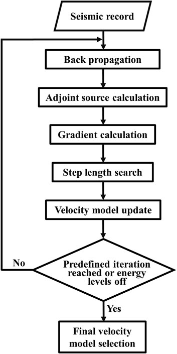
FIGURE 1. The workflow of WEFT for passive source tomography.

Numerical Tests

To validate WEFT, we perform a series of synthetic tests using heterogeneous models in 2D. The true velocity model (Figure 2A) used for the following numerical experiments is adapted from the widely used Marmousi model (Martin et al., 2002). Both the true and smooth initial velocity models (Figures 2A,B) are from Schuster (2017). A Ricker wavelet with central frequency of 15 Hz is chosen as the source time function. The source-receiver configuration consists of 201 receivers on the surface with an interval of 20 m, and 31 passive sources located in the subsurface (Figure 2). These sources are distributed into 6 clusters. We should emphasize that the synthetic model used here is for the proof of concept for the proposed WEFT method and may not follow the actual scenarios for earthquake monitoring. However, with more and more dense seismic arrays used for monitoring induced seismicity, the distribution of dense receivers and shallow passive seismic sources are actually expected, such as the dense geophones used for monitoring shale gas hydraulic fracturing (Eisner et al., 2010; Staněk and Eisner, 2013; Anikiev et al., 2014).

FIGURE 2

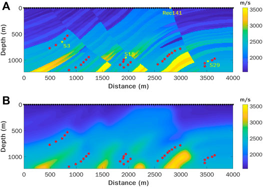
FIGURE 2. 2D velocity models used for synthetic tests with WEFT. (A) The true model adapted from the Marmousi model. (B) The initial model used for WEFT. The inverted triangles at the top of the model denote the 201 receivers with an interval of 20 m, and the asterisks within the model denote the 31 earthquake sources. The yellow asterisks and the yellow inverted triangle indicate the sources and receiver used for the data comparison in Figure 8.

Following the approach now commonly used in FWI, which sequentially utilizes observed data with increasing frequencies (Bunks et al., 1995), a multiscale strategy is also adopted in WEFT. After a predefined number of iterations is reached for a certain frequency band, the final velocity model is used as the initial model for the next frequency band. Since the source location used in this case is accurate, we choose a small spatial aperture $l_{x} = l_{z} = 40 m$ , and the temporal aperture is larger than the half-width of the source wavelet. To improve the resolution of the inverted model, the spatial aperture $l_{x, z}$ in Eq. 7 for evaluating the focused energy is gradually decreased with increasing frequencies. We first test the WEFT using passive seismic sources with a uniform radiation pattern (indicated by the small adjacent ring in Figure 3A). Four frequency bands of 1–5 Hz, 1–9 Hz, 1–16 Hz, and 1–28 Hz are adopted. It can be seen that the inverted model (Figure 3A) is hardly affected by the source radiation pattern although the source moment time function is not provided for the inversion. The focused energy (Figure 3B) increases with iterations in each frequency band and its growth levels off gradually. Meanwhile, the model misfit measured by the L2-norm also decreases with iterations, as shown in Figure 3C.

FIGURE 3

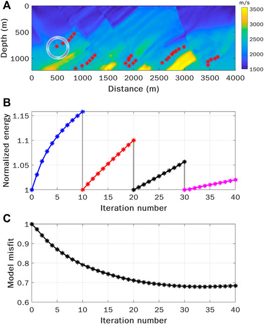
FIGURE 3. Velocity inversion with WEFT using passive sources with a uniform radiation pattern. (A) The inverted velocity model by WEFT using the multiscale strategy. The source radiation pattern is indicated by the small adjacent ring. (B) The focused energy with iterations at the source locations. For the focused energy, their values are renormalized by the respective values at the first iteration in every frequency band (indicated by different colors). Waveforms in four frequency bands, 1–5 Hz, 1–9 Hz, 1–16 Hz, and 1–28 Hz are sequentially used for updating the velocity model, with 10 iterations in each band. (C) The normalized model misfit measured by L2-norm as a function of iterations.

We further test a more complicated scenario where six seismic clusters having different types of source moment tensors (Figure 4A). The spatialtemporal aperture used here is the same as in the previous case. The model inverted by the multiscale WEFT is shown in Figure 4B. Though the varying radiation patterns from different clusters pose a considerable challenge for waveform inversion, WEFT still inverts for the heterogeneous Marmousi model accurately. Compared to the true model, there are some minor artifacts in the inverted model, which are probably caused by the varying radiation patterns that can result in complicated directional illuminations in resolving the model. Although the stacking energy (Figure 4C) increases with iteration in each frequency band as expected, the model misfit (Figure 4D) undesirably also increases slightly in the last frequency band, which suggests the inversion was trapped in a local minimum for high-frequency data. Nevertheless, this example demonstrates that WEFT can be applied directly to surface seismic monitoring datasets in which seismic sources occur on different faults are with varying orientations and slipping angles.

FIGURE 4

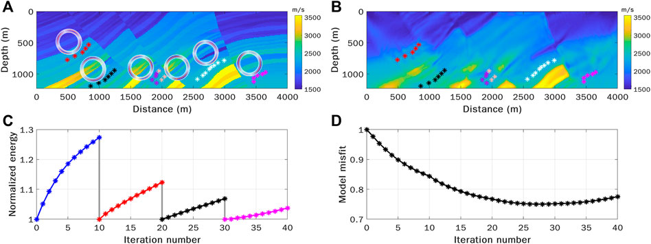
FIGURE 4. Velocity inversion with WEFT using passive sources with varying radiation patterns. (A) Distribution of six seismic clusters (colored asterisks), each of which has a distinct radiation pattern indicated by small adjacent rings. The true velocity model is shown in the background. (B) The model inverted by multiscale WEFT with seismic sources in (A). (C)The focused energy with iterations at the source locations. (D) The normalized model misfit measured by L2-norm as a function of iterations.

Discussions

Influence of Uncertainty in Source Location

In WEFT, the source location is used to determine the spatial volume for evaluating the focused energy (Equation 7), and for the adjoint source injection when calculating the adjoint wavefield ( $λ_{p}$ in Equation 15). As discussed earlier, in WEFT it is assumed that the source location and origin time are predetermined from other methods, e.g., the NonLinLoc method (Lomax et al., 2000), the double-difference location method based on traveltimes (Waldhauser and Ellsworth, 2000; Zhang and Thurber, 2003), or the recently developed location methods based on machine learning (Kriegerowski et al., 2019; Zhang et al., 2020; Wang and Alkhalifah, 2021). Thus, the source location may deviate from its true position owing to an inaccurate velocity model (Thurber, 1992) and arrival times. In WEFT, a way to mitigate the influence of inaccurate source locations is to expand the spatial aperture for evaluating the focused energy (determined by $l_{x}$ and $l_{z}$ in Equation 7). That is, the spatial aperture should be designed based on the source location uncertainty so that the true location is contained in the volume for evaluating the focused energy. To some extent, however, this strategy may also compromise the accuracy and resolution of the inverted velocity model, since the back-propagated wavefields using a slightly incorrect model may still focus well within an enlarged volume. When the source locations are known accurately, the inverted model using a smaller spatial aperture with $l_{x} = l_{z} = 4$ 0 m is shown in Figure 5C, and the model misfit is reduced by about 30%. However, when the source locations are not accurate, the result using the same spatial apertures shows a slightly distorted inclined high-velocity layer at the bottom of the model $(x \approx 3000 m, z \approx 1000 m)$ and a blurred inclined thin layer with low velocity $(x \approx 3000 m, z \approx 600 m)$ (Figure 5A). The model misfit in this case is only reduced by 10%. If we enlarge the apertures to $l_{x} = l_{z} = 100 m$ , not only the model misfit is reduced by about 18% of the original, but also the distortion is suppressed and the low-velocity thin layer is better recovered (Figure 5B). By comparing models in Figure 5A,B,C, we notice that some artifacts around the sources are introduced with inaccurate source locations.

FIGURE 5

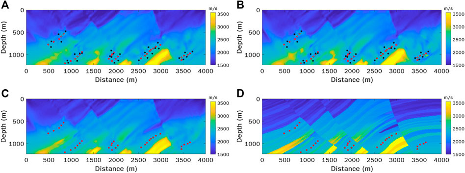
FIGURE 5. Comparison of the velocity inversion results with different focusing apertures and with or without source location errors. (A) The model inverted with the smaller apertures ( $l_{x} = l_{z} = 40 m$ ) while the source locations (black asterisks) deviate from their correct positions (red circles). (B) The model inverted with larger apertures ( $l_{x} = l_{z} = 100 m$ ) under the same conditions as (A). (C) The model inverted with smaller apertures as (A) when source locations are accurate (red asterisks). (D) The true model for comparison.

Comparison With Full Waveform Inversion and Seismic Travel Time Tomography

Since WEFT evaluates the magnitudes of the back-propagated energy focused around the hypocenters instead of matching the wiggles between the observed and synthetic waveforms at the receivers, the proposed method has less nonlinearity and is more robust since there is less cycle-skipping issues as commonly seen in conventional FWI. Figure 6B shows a comparison of objective functions of FWI and WEFT for a simple source-receiver configuration (Figure 6A), where the passive source is located at 1,000 m in depth and a single receiver is on the surface. It is obvious that the objective function of FWI has multiple local minima compared to that of WEFT, which has a more convex behavior globally and has only a single global minimum for this scenario.

FIGURE 6

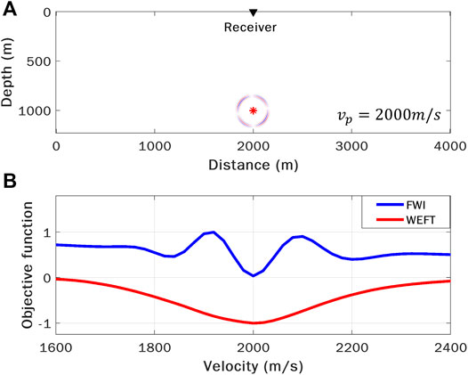
FIGURE 6. Comparison of the objective functions between FWI and WEFT. (A) The source-receiver configuration used for calculating the objective functions. The source radiation pattern is indicated by the small adjacent ring. The velocity model is homogenous with Vp equal to 2000 m/s. (B) Comparison of the normalized objective functions for FWI (blue) and WEFT (red) with respect to different velocities.

The lower nonlinearity of WEFT can also facilitate velocity inversion from a poor initial velocity model. In Figure 7, we further compare the inversion results between WEFT and conventional traveltime tomography using an even smoother initial velocity model (Figure 7A). Compared to the true model, many small heterogeneities and contrasts are recovered in the inverted model by WEFT (Figure 7C), while only the tilted high-velocity bodies at the bottom of the model are distorted. In comparison, the inverted model by traveltime tomography (Figure 7B) appears much smoother and lack fine details. Starting from the final inverted model from WEFT, we perform FWI to further update the velocity (Figure 7D), and even more details are added to the model. It should be stressed again that WEFT does not require source moment time functions in the inversion, while FWI does. Using the final velocity models inverted by WEFT and traveltime tomography shown in Figure 7, we generate synthetic waveforms and compare the $v_{x}$ and $v_{z}$ components (Figure 8). Significant time delays can be found between the “observed” data from the true model (black lines) and the ‘synthetic’ data generated based on the initial model (blue lines). Although the model inverted by traveltime tomography considerably mitigates the time delays between the observed and synthetic data, wiggles in the two datasets still differ markedly. In comparison, the waveform matching between the synthetic and observed data improves considerably using the velocity model derived by WEFT, with many later-arrived wiggles successfully modeled. When using the model inverted by FWI starting from the final model of WEFT, the synthetic and observed waveforms are almost the same. This nice agreement in waveforms indicates that though the objective function of WEFT only considers the energy focusing at the sources directly, the waveform matching at the receivers is nevertheless satisfactory owning to a correctly updated model.

FIGURE 7

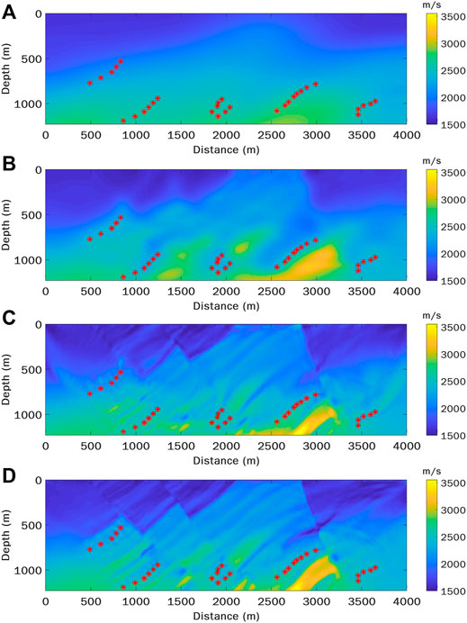
FIGURE 7. The inverted models using traveltime tomography and WEFT from a rather smooth initial model. (A) The rather smooth initial model. (B) The model inverted by traveltime tomography. (C) The model inverted by multiscale WEFT. (D) The model further inverted by multiscale FWI starting from the WEFT model in (C).

FIGURE 8

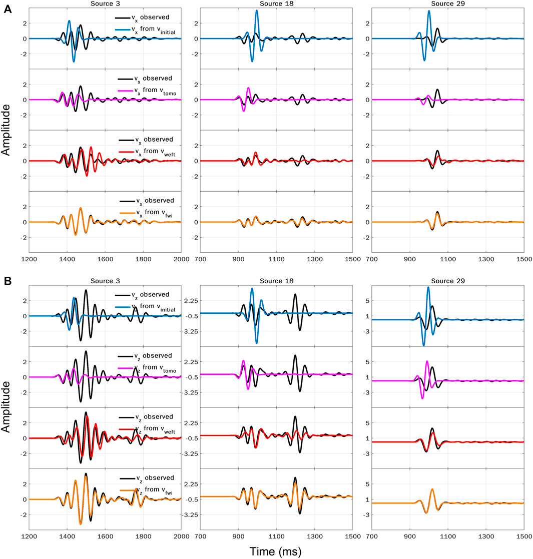
FIGURE 8. Comparison of waveforms for the (A) $v_{x}$ and (B) $v_{z}$ components at a particular receiver from different sources using various velocity models. The black lines denote the observed data. The blue, magenta, red and orange lines denote the synthetic data with the initial model (Figure 7A), the final velocity models from traveltime tomography (Figure 7B), WEFT (Figure 7C) and FWI (Figure 7D), respectively. The subplots in each column show data from a different source. The locations of the receiver (yellow triangle) and the sources (yellow asterisks) are shown in Figure 2A. The waveforms are filtered between 1 and 28 Hz, and the true source moment time functions are used.

Influence of Noise

We further test the stability and accuracy of WEFT with noisy observed data (Figure 9A). In this experiment, the synthetic data are contaminated by random Gaussian noise, which is not coherent among receivers, and the SNR is about 0.3. For the noisy data, it is difficult to obtain a relatively accurate velocity model by conventional FWI without sophisticated data preprocessing. However, it is still possible to apply WEFT with the noisy data. This is because although the seismic signals are initially buried in the noise, the coherent signals can be gradually enhanced against the inherent noise with back-propagation. In other words, wavefield back-propagation specifically focuses the energy of the microseismic event and thus suppresses incoherent noise, which can be seen in the snapshots of the back-propagated wavefields at a certain time with noise-free and noisy data (Figures 9B,C, respectively). Compared with the inverted model from the noise-free data (Figure 3), the inverted model with the noisy data is similar (Figure 10A), and the model misfit (Figure 10C) still shows a considerable reduction. This test demonstrates that WEFT is rather resilient to incoherent noise, which can be a considerable advantage over FWI.

FIGURE 9

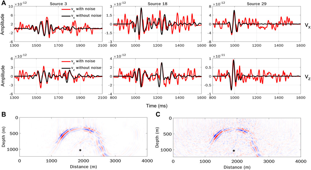
FIGURE 9. The comparison between the noisy and noise-free synthetic data used for WEFT. (A) Noisy and noise-free traces at selected receivers. The source radiation pattern is the same as that shown in Figure 3. The black lines indicate the noise-free data, and the red lines indicate the noisy data by superposing the noise-free data with random Gaussian noise with limited bandwidth. The distributions of the sources and receivers are the same as those shown in Figure 2. (B) and (C) show the snapshots of the back-propagated wavefield with noise-free and noisy data, respectively.

FIGURE 10

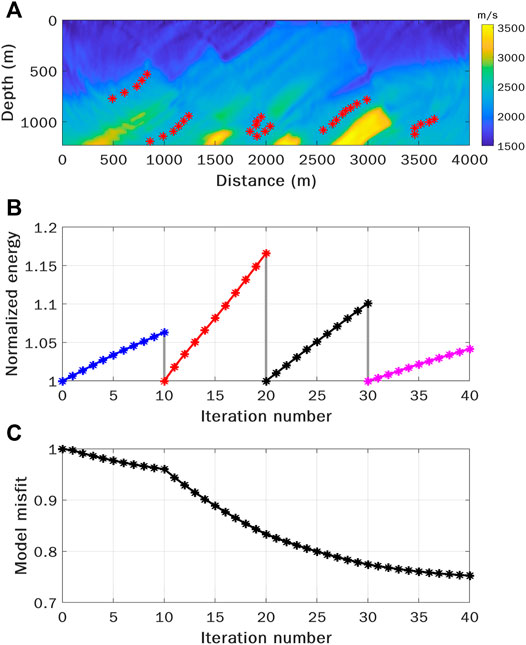
FIGURE 10. Results of multiscale WEFT using data with random Gaussian noise with limited bandwidth. (A) The inverted velocity model with multiscale WEFT. (B) The focused energy with iterations at the source locations. The parameters used in the inversion are similar to those used in Figure 3. (C) The normalized model misfit measured by L2-norm as a function of iterations.

Influence of Source Distribution

Considering that the distribution of sources and the source mechanisms may have a noticeable influence on the inverted model, we further perform a challenging test where 10 earthquakes with a uniform radiation pattern are distributed within a narrow depth range of 60 m, as shown in Figure 11A. Starting from the initial model shown in Figure 11B, two distinct source mechanisms are used for comparison. The inverted models using sources with different radiation patterns (indicated by the small adjacent ring) are shown in Figures 11C,E, respectively. The comparison of the velocity profiles at the position x = 2,310 m is shown in Figures 11D,F, respectively. We found that, as expected, most of the effective update is within the central part of the model above the earthquake sources due to the limited source illumination. Besides, different source mechanisms, which result in varying illumination patterns, inevitably have an impact on the inverted models. Due to the poor source distribution, the recovered models are not as good as those shown before. However, both inverted models are updated successfully compared to the initial one, especially the model shown in Figures 11C,D.

FIGURE 11

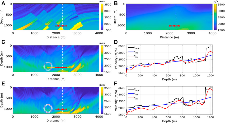
FIGURE 11. Comparison of the velocity inversion results using clustered earthquakes in a narrow depth range with uniform focal mechanisms. (A) The distributions of 10 sources (red asterisks) and 199 receivers (black inverted triangles) with the true model in the background. (B) The initial model used for WEFT. (C) and (E) are the inverted models using sources with two distinct focal mechanisms (indicated by small adjacent rings). (D) and (F) are the corresponding comparisons of the true (black), initial (blue) and inverted (red) velocity profiles at x = 2,310 m (indicated by a white dash line).

Conclusion

We propose a new seismic tomography method called Waveform Energy Focusing Tomography for passive seismic sources. Compared to FWI, WEFT inverts for the velocity model by maximizing the energy of the moment time functions from back-propagated wavefields around the sources, instead of matching synthetic and observed waveforms at the receivers. As a result, WEFT has lower nonlinearity in the inversion and can avoid the cycle skipping issue in FWI. More importantly, except for the source locations and origin times, WEFT does not require other source attributes including source time functions and focal mechanisms. This means that more earthquakes with smaller magnitudes and unknown source mechanisms can also be used by WEFT.

We have shown the effectiveness and advantages of WEFT through several 2D synthetic tests based on the Marmousi model. WEFT can still perform well on different challenging cases when passive seismic sources have different radiation patterns, when the initial velocity model is rather smooth, and when waveforms are very noisy. Nevertheless, the quality of inverted models can still be affected by uneven illumination due to distributions and mechanisms of sources. Although waveform matching at the receivers is not directly considered in the objective function of WEFT, the synthetic tests show that the waveform matching using the inverted model by WEFT is still satisfactory, much better than the velocity model inverted by traveltime tomography using arrival times. It should be noted that WEFT yields velocity models with slightly lower resolution compared to FWI. Therefore, WEFT can act as an intermediate step between seismic traveltime tomography and FWI by providing a more accurate and reliable starting velocity model for the latter.

In this study, for simplicity we validate WEFT with passive seismic sources under the 2D acoustic assumption. This method can also be extended to 3D for real applications such as dense-array monitoring of local seismicity from fault zones or hydraulic fracturing when the receivers are not distributed along a straight line or the passive sources have an areal distribution, which will be shown in a future study.

Data Availability Statement

The raw data supporting the conclusions of this article will be made available by the authors, without undue reservation.

Author Contributions

YH, JL, and HZ all contributed to the study. YH performed the numerical tests and wrote the first draft of the manuscript. All authors contributed to the revision and approved the submitted version.

Funding

This research is supported by the National Natural Science Foundation of China under grants 41961134001 and 41874048, and supported by the National Key Research and Development Projects 2021YFC3000602 and 2018YFC1504102.

Conflict of Interest

The authors declare that the research was conducted in the absence of any commercial or financial relationships that could be construed as a potential conflict of interest.

Publisher’s Note

All claims expressed in this article are solely those of the authors and do not necessarily represent those of their affiliated organizations, or those of the publisher, the editors and the reviewers. Any product that may be evaluated in this article, or claim that may be made by its manufacturer, is not guaranteed or endorsed by the publisher.

Acknowledgments

The authors would like to thank Haipeng Li for his many helpful discussions. We also thank two reviewers and editor Tariq Alkhalifah for their very helpful comments in improving our manuscript.

References

Adamczyk, A., Malinowski, M., and Górszczyk, A. (2015). Full-waveform Inversion of Conventional Vibroseis Data Recorded along a Regional Profile from Southeast Poland. Geophys. J. Int. 203, 351–365. doi:10.1093/gji/ggv305