 Hanwen Jia1,2
 Baoxu Yan
 Kai Guan
94% of researchers rate our articles as excellent or good
Learn more about the work of our research integrity team to safeguard the quality of each article we publish.
Find out more
ORIGINAL RESEARCH article
Front. Earth Sci. , 09 May 2022
Sec. Geohazards and Georisks
Volume 10 - 2022 | https://doi.org/10.3389/feart.2022.897779
This article is part of the Research Topic Advanced Application of Deep Learning, Statistical Modelling, and Numerical Simulation on Geo-Environmental Hazards View all 59 articles
Evaluation of the stability of a shallow goaf in an open-pit iron mine is important for successful mining. Based on the idea of “rock disaster analysis and prediction combining field monitoring and numerical simulation,” a modification of Mathews stability graph is proposed, and a monitoring scheme combing stress, displacement, and surface subsidence is selected per the field geological condition. The displacement monitoring data and numerical model are combined, and the numerical model is corrected per the monitoring data; the time-dependent deformation and damage to the goaf is obtained; and its stability is comprehensively evaluated. Results show that the northern area is in a relatively stable stage, whilst the southern area has a certain risk of collapse. At last, the proposed framework was successfully used in the open-pit iron mine to evaluate the stability of the shallow goaf and can be used for reference to similar geological conditions.
The prediction method of underground space stability and its lifetime assessment is a hot issue in the mining industry, tunnel excavation, and railway construction in recent years. The failure rock mass has a critical potential to cause workers to be buried, equipment damage, and tunnel blockage (Cui et al., 2021; Xsa et al., 2021; Zhou et al., 2021), and the shock waves can cause direct casualties (He et al., 2010). Moreover, rock failure may also destroy the aquifuge and lead to water inrush or permeable accidents (Kuscer, 1991). The large-scale collapse in shallow ground results in direct damage to surface buildings and casualties (Zhang et al., 2015), even the landslides, collapses, and surface water recharge (Tang et al., 2019; Li et al., 2022). Factors affecting the stability of underground space mainly include the natural hydrogeological conditions, such as buried depth, dip angle, thickness, and lithology of overlying strata, and human factors, such as operation method, blasting disturbance, and excavation times (Li et al., 2021a; Li et al., 2021b). The commonly used stability analysis and prediction and prewarning methods can be roughly divided into three categories: theoretical analysis method, prediction method based on monitoring threshold, and numerical simulation method.
Theoretical or empirical formula analysis methods mainly include elastic mechanics theory, catastrophe theory mathematical model method, and Mathews stability graph method (Jia et al., 2020). Many researchers use the elastic mechanics method to simplify the roof of underground space to an ideal elastic body such as Pu’s theoretical model, thin plate model, and moderate thick plate model. Solving the internal stress of goaf roof by applying boundary conditions, furthermore, to analyze its stability (Nomikos et al., 2002; Chen et al., 2020; Sun et al., 2021). The main purpose of catastrophe theory is the phenomenon and law of a stable configuration transition to another configuration. Researchers introduce catastrophe theory into the study of instability and failure, which could solve the failure mechanism and mode of underground chamber roof, rock pillar, or ore pillar from stable to unstable (Han et al., 2019; Xia et al., 2019; Qiao et al., 2021; Wang X. et al., 2021). The failure process of underground space is a highly nonlinear risk. Therefore, more and more researchers start to investigate the internal relationship between data factors through mathematical calculation and establishing appropriate mathematical instability criterion model, which includes neural network model, genetic mathematical model, and fuzzy mathematical model (Majdi and Beiki 2010; Sidorenko et al., 2021; Zhang et al., 2021). Mathews proposed the Mathews stability graph method (Mathews et al., 1981), and it is a rock classification system based on practice, which is relatively simple and convenient for field implementation. However, Potvin improves the stability graph by modifying the stability number N and adding a transition region to simplify it to a stable zone, transition zone, and caving zone (Potvin 1988). Based on the requirements of support system condition, fault occurrence, stope dilution rate, and instability probability, researchers purpose a new Mathews stability graph, respectively (Nickson 1992; Clark and Pakalnis 1997; Suorineni 1998; Mawdesley et al., 2001; Mawdesley 2004; Suorineni 2010). According to different conditions of rock stress factor, scholars have carried out corresponding corrections by numerical calculation, theoretical analysis, mathematical model, and field measurement, which have achieved good results in engineering (Stewart and Trueman 2001; Bewick and Kaiser 2009; Mitri et al., 2011; Vallejos et al., 2018; Jia et al., 2020). For rock materials, the tensile strength is much lower than the compressive strength, so it is necessary to estimate the instability caused by tensile failure of rock mass, which is ignored in the current Mathews stability graph method, and the multidimensional stress state of the surrounding rock is not considered in the calculation process of the rock stress factor.
Prediction and prewarning method based on monitoring parameter threshold refers to the real-time prewarning of disasters when the reasonable range of monitoring data is determined artificially by empirical analysis, theoretical analysis, or engineering analogy. In general, the “point” monitoring or the “field” monitoring will be adopted. The “point” monitoring mainly includes internal stress monitoring, surface displacement monitoring, and internal displacement monitoring of rock mass (Yang et al., 2021; Yi et al., 2021; Zhu et al., 2021), whilst the “field” monitoring generally includes microseismic monitoring and electromagnetic radiation monitoring (Tang et al., 2010; Ge 2005; Wang J. X. et al., 2021). The selection of the prediction index plays an essential role in this method (He and Kusiak, 2017). Not only the magnitude of the index can indicate whether the surrounding rock deformation is in the accelerated stage but also different prediction indexes represent different characteristics of surrounding rock deformation. However, there are still three deficiencies in the prediction and prewarning processing based on field data: 1) The disaster-causing process and evolution mechanism of the engineering site are not clear. 2) Data quality has a strong dependence. 3) Onsite monitoring is mostly point monitoring, which is unable to achieve full coverage.
In addition to the prediction and prewarning methods mentioned above which are based on the field monitoring data, numerical simulation methods are often used to analyze and evaluate the possibility of rock mass disasters. According to different numerical solution methods, they can be divided into finite element, discrete element, boundary element, meshless method, DDA, manifold element, and other methods (Shi 1988; Ohnishi et al., 2014; Chen 1998). It is more convenient to analyze the disaster-causing process of rock mass with the assistance of numerical simulation. On this basis, the analysis and prediction of the evolution of the damage zone can also be realized, providing a critical theoretical and technical support for disaster prediction and prewarning (Müller 1991; Rouabhi et al., 2005). Moreover, the numerical simulation method is able to demonstrate the mechanical response state of the research area directly, which provides a theoretical basis for interpreting monitoring data and mining precursor characteristics. It provides an important reference for researchers to understand the mechanism and development law of disasters. Jiang et al. (2019) predicted the deformation and failure depth of surrounding rock of an underground chamber by combining a bionic particle swarm algorithm with numerical calculation. Based on the numerical calculation, Habibi analyzed the long-term stability of salt caverns with different shapes, sizes, and depths under cyclic loading of 3∼8 MPa (Habibi et al., 2021). Current numerical simulation methods are based on the previous exploration data and cannot carry out the real-time dynamic numerical simulation based on different field condition, which cannot achieve the real-time performance of prediction and prewarning.
As for the stability analysis and prediction prewarning of underground engineering, the empirical theoretical method, field monitoring method, and numerical simulation method mentioned above have their own unique advantages; meanwhile, the shortcomings of these methods cannot be ignored. If existing methods can be effectively combined, the efficiency of prediction and prewarning of hazards in underground engineering can be greatly improved. Therefore, taking the goaf area of an open-pit iron mine as the engineering background, considering the influence of spatial multidimensional stress on rock stress factor A, the Hoek–Brown criterion with tensile truncation is used to correct the rock stress factor A, and the Mathews stability graph will be optimized. Based on the idea of a “rock disaster analysis and prediction method combining field monitoring and numerical simulation,” the monitoring data and numerical simulation results are fused, and the creep damage calculation implemented in FLAC3D is carried out by dynamic feedback based on the field measured multipoint displacement data. Combined with the damage evolution law obtained by real-time numerical simulation, the deformation damage and failure trend of goaf are predicted. Then, the stability of goaf is comprehensively evaluated according to the combination of field monitoring, numerical simulation, and theoretical analysis.
The open-pit iron mine is located in the east of Anshan, Northeast of China (E 123°30′00″, N 41°07′40″), which owns three mining areas of Hejia, Dumu, and Dalazi as shown in Figure 1. Because of the historical reasons, the open-pit iron mine has experienced mining activity in the early stage, especially the irregular mining and disorderly excavation of local small mines, which results in many underground goaf areas. With the expansion and extension of the mining activity, those areas in the Dumu mining area have brought significant threats to normal production. Meanwhile, it also accompanies critical difficulties in the exploitation and utilization of deep iron ore resources and the implementation of mining engineering plans. At the same time, the goaf area is a serious threat to the safety of large-scale equipment in mines, and it also causes serious security risks to the blasting quality and blasting safety of mines. For example, on 15 April 2016, the No. 13 drilling rig located at E-4049.458, N-242.721m, and H-209.8 m in the outer extension area of Dumu, forming a collapse pit of about 45 m along east–west, 44 m along north–south, 1,499 m2 in area, and 7m in surface subsidence. On 5 May 2016, in Dumu mining area E-3426.508 m, N-373.914, and H-158.4m formed about 3.2 m in east–west, about 2.9 m in north–south length, 8 m2 area, and 0.1 m subsidence area.
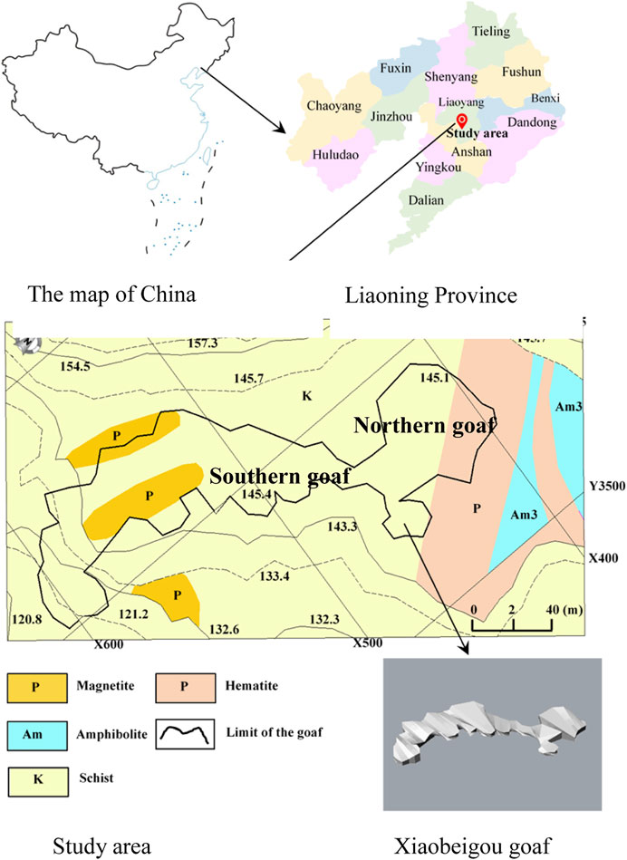
FIGURE 1. The field map of hydrostatic leveling system for the open-pit iron mine.
At present, there are six production levels in Dumu mining area, with the highest production level of +292 m, and the lowest production level being +120 m. Four iron layers are located in the mining area: Fe1, Fe2, Fe3, and Fe4. Meanwhile, Fe2 occupies the largest thickness of 34 m. The lowest ore body is Fe1, with Fe4 locating the highest position. There are rock interlayers between the ore layers, and the average thickness of the rock layer is 25 m. The Fe4 ore layer is 150 m away from the surface, which is covered with rock mass. The dip angle of the ore body is 8–25°, the average geological grade is 32.42%, the ore weight is 3.3 t/m3, and the rock weight is 2.6 t/m3. The goaf in the Xiaobeigou area of Dumu mining area is located in the +145 m platform, which is divided into two areas: the first area is the northern goaf, its length is about 65 m, width is about 48 m, height is about 6 m, and the thickness of the roof is between 20 and 26 m, while for the roof slag is between 2 and 3 m. The second is the southern goaf area, which is about 130 m in length, 40 m in width, and about 5 m in height. The thickness of roof is from 12 to 20 m, and the thickness of the roof slag is about 5 m.
Potvin illustrates the stability graph method based on the calculation of the hydraulic radius HR in the critical surface and the modified stability number N′. These two factors were plotted on the graph which is divided into the stable zone, transition zone, and the caving zone, so as to express the stability of the underground excavation area (Potvin 1988). The hydraulic radius HR in the stability graph can be obtained using Eq. 1:
The stability number N′ (Potvin 1988) is calculated by Eq. 2:
where
where RQD is the rock quality index,
Parameter B in Eq. 1 is the joint adjustment factor, and its value is measured by the difference between the dip angle of the mining face and the main joint set, which is shown in Figure 2A. Parameter C is the gravity adjustment factor, which is related to the failure mode of the goaf under gravity, which is shown in Figure 2B below.
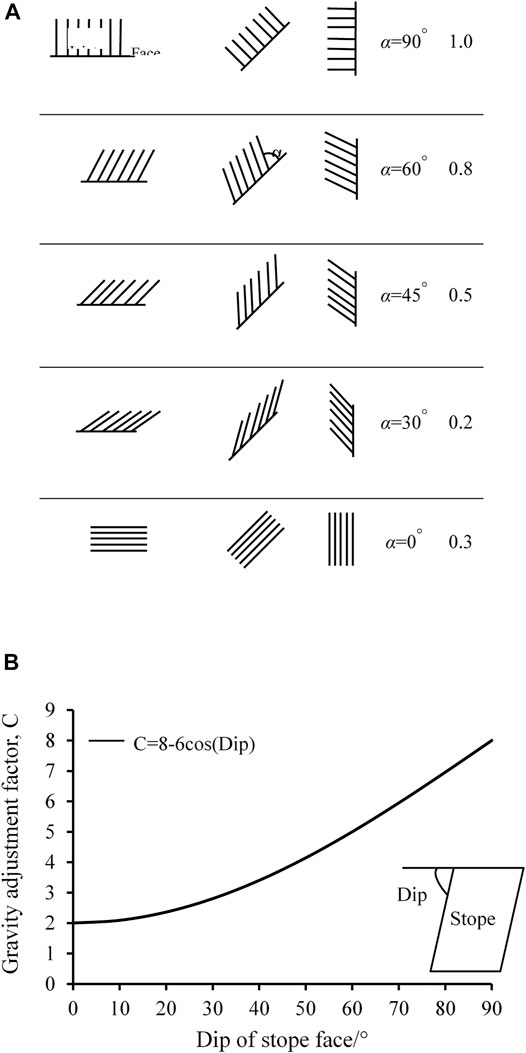
FIGURE 2. (A) Joint orientation adjustment factor B and (B) cavity adjustment factor (C).
A is the rock stress factor, which is calculated by the ratio of the uniaxial compressive strength (UCS) in intact rock to the compressive stress σ1max is the maximum induced tangential stress acting at the center of the critical face. The value of A is linearly related to UCS/σ1max, and its range is 0.1–1. It is calculated by the following Eqs. 4 and 5:
It can be seen from Eq. 5 that the Potvin modified graph method believes that the stope will be in a stable state under low-stress state (when 10 < R). At this time, the obtained A is the maximum, which leads the calculated stability number N’ to the maximum value. By accounting for the adverse relaxation effect in the stope under low stress (10 < R), Mitri et al. (2011) revised the calculation method for A by introducing the maximum stress factor (MSF) at the center of the critical face:
In the widely used (Potvin (1988) and Mitri et al. (2011)) modified graph method, Eqs 4, 5 of stress factor
1) The stress state at any point in the plane is determined by the maximum principal stress
(2) The calculation formula of
According to the aforementioned two problems, this article uses the modified Hoek–Brown criterion with tensile cut-off (Dai et al., 2018) as the judgment basis for rock mass engineering instability. The Hoek–Brown criterion is demonstrated by Hoek and Carranza-Torres, 2002, who statistically analyze a larger number of rock-triaxial test data and rock field test results, comprehensively considering the influence of the rock-mass structure, rock strength, stress state, and other aspects to obtain the empirical formula of the rock mass failure, which can reflect the inherent nonlinear failure characteristics of rock mass. Therefore, this criterion is widely used in underground chambers, slopes, tunnels, and other engineering projects in the rock engineering sector. Hoek–Brown criterion with tensile cut-off is shown as follows (Dai et al., 2018):
where σ1 is the maximum principal stress of rock mass failure,
Based on the MSF calculation method proposed by Mitri et al. (2011) and the Hoek–Brown criterion with tensile cut-off (Dai et al., 2018), the MSFc calculation under shear failure mode is modified according to Eq. 13, and the MSFt calculation under tensile failure mode is added according to Eq. 14:
In Eqs 13 and 14, MSFc is the maximum stress factor upon shear failure in the critical face of the stope, MSFt is the maximum stress factor upon tensile failure in the critical face of the stope,
When
When
where
It is worth to explain that the tensile strength of the rock mass is much smaller than the compressive strength. For this reason, this article gives priority to judge the tensile failure when solving the stress factor. By distinguishing
When
In order to obtain the evolution characteristics of stress and displacement of the roof in the northern goaf of Xiaobeigou, combined with the geological data in the northern goaf of Xiaobeigou and the thickness distribution of the roof in this area, a group of four-point bolt dynamometers and two-point multipoint displacement meters are arranged in each area of A and B in the northern goaf for real-time monitoring of stress and displacement. The sensor measurement method is 24-h automatic uninterrupted monitoring. The layout plane position of the measuring points is shown in Figure 3. The green measuring point in the figure represents the layout position of the multipoint displacement meter, whilst the red measuring point represents the layout position of the bolt dynamometer.

FIGURE 3. Layout plan of monitoring points.
The depth of holes A and B for the bolt dynamometer is about 21 m. The first force sensor is about 7.7 and 7.4 m from the vertical distance to the goaf roof, respectively. Meanwhile, each force sensor is arranged every 3.5 m to complete the layout of the two sets of bolt dynamometers. The depth of holes A and B of the multipoint displacement meter is about 21 m, and the first measuring point is arranged at the bottom of the hole. The first measuring point of hole A is about 7.2 m away from the roof of the goaf, and the second measuring point is about 11.2 m away from the roof of it. The first measuring point of hole B is about 3.4 m away from the roof of the goaf, and the second measuring point is about 7.4 m away from the goaf roof.
Since the establishment of the bolt dynamometer monitoring system in Xiaobeigou goaf on 6 June 2018, it has been running well except for the signal loss caused by the equipment failure of hole B from July 29 to 31 August 2018. All-weather monitoring of rock stress around the goal of Xiaobeigou is realized. The stress variation characteristics of the monitoring points of holes A and B with time are shown in Figures 4A,B. In this figure, the fluctuation amplitude of the A4 point is large, with a fluctuation amplitude of about 0.3 MPa. The distance between the A4 measuring point and the surface is about 2.7 m. Affected by the external environment such as the surface engineering equipment operation and the uneven stress distribution of shallow surface soil caused by rainfall, the measuring point has a wide range of fluctuations. On August 2 (53 days of monitoring period), the stress increase rates from measuring points A1 to A3 were 0.003 MPa/d, 0.004 MPa/d, and 0.002 MPa/d, respectively. Subsequently, it increased to 0.005 MPa/d, 0.006 MPa/d, and 0.003 MPa/d, respectively. The maximum stress value of the bolt dynamometer in hole A was 0.51 MPa. Due to the damage of environmental factors, the maximum stress of the B3 measuring point is 0.61 MPa during the monitoring period. The stress values of 8 measuring points from hole A and hole B are small, but they are all in the stress acceleration stage.
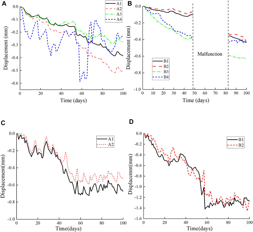
FIGURE 4. Variation characteristics of stress with time at each measuring point of (A) hole A and (B) hole B and displacement with time at each measuring point of (C) hole A and (D) hole (B).
Since the establishment of the bolt dynamometer monitoring system in Xiaobeigou goaf on 6 June 2018, the system has been running well, and the all-weather monitoring of roof rock mass displacement around the goaf of Xiaobeigou has been realized. The displacement of the monitoring points holes A and B with time is shown in Figures 4C and D.
Till June 24 (14 days of monitoring period), the displacement from measurement points A1 to A2 subsidence to 0.27 and 0.23 mm, with the rate of 0.019 mm/d and 0.016 mm/d, respectively. It started to sink for the second time on the 29th day (after 15 days of the quiet period), with the subsidence rate of 0.022 mm/d and 0.019 mm/d, respectively. On August 5, it went into the second quiet period, showing a “deformation period–quiet period–deformation period–quiet period” characteristic.
Till July 4, the displacement from measuring points B1 to B2 sank to 0.61 and 0.55 mm respectively, with the subsidence rates of 0.025 mm/d and 0.023 mm/d. It experienced the second sink on the 35th day (after 11 days of the quiet period), with a subsidence rates of 0.035 mm/d and 0.029 mm/d, respectively. It reached the second quiet period on August 10, and similar to the deformation rules of hole A, it showed a “deformation period–quiet period–deformation period–quiet period” characteristic. However, the deformation value of hole B is about 1.9 times of hole A, and the roof subsidence rate is also greater than hole A. Hole B is located in the ore-rock interface, and there is a lithologic interface, so the roof stability is poor.
The hydrostatic leveling system (HLS) is composed of a data acquisition terminal, sensor, power supply, and data transmission line, hydraulic line, and cloud data server. The hydraulic line part is mainly composed of a liquid pipe and a liquid storage tank. The liquid storage tank and each sensor are connected in series through the liquid pipe to form a connector. The first sensor connected with the liquid storage tank is set to avoid surface settlement. The settlement value of other measuring points can be determined by the change in liquid pressure of the sensor. The SD-226 hydrostatic leveling monitoring system produced by Shanghai Shengdi Sensor Technology Co., Ltd. was selected for this surface subsidence monitoring. The measurement method of the sensor is 24-h automatic uninterrupted monitoring, and the surface vertical displacement data are collected every 5 minutes. According to the principle of mining hydrostatic leveling measurement, the first measuring point is taken as the reference point and 12 leveling measuring points are arranged along the main section of the mining subsidence basin by the “line” layout. As shown in Figure 5, red points are the measuring points of hydrostatic leveling.
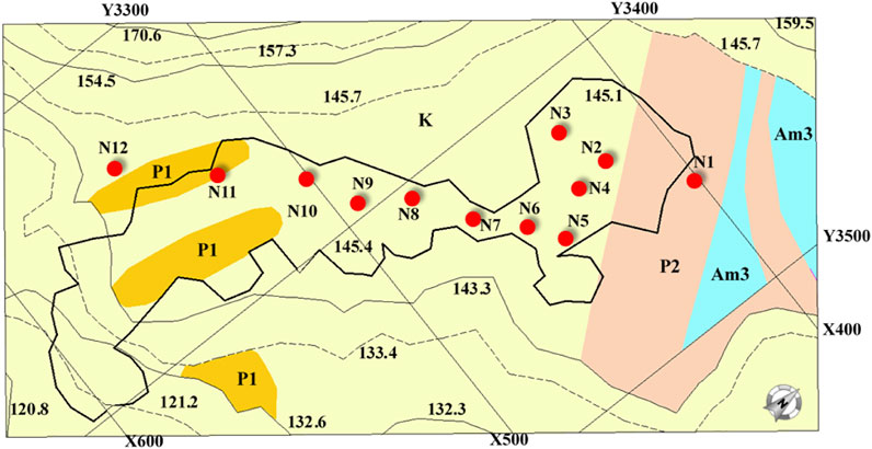
FIGURE 5. Detailed arrangement scheme of the HLS.
The roof thickness of the shallow goaf area located in Xiaobeigou is small, which results in the small subsidence of the surface during the collapse process. In addition, the elevation difference in most areas of the +145 m platform is small (about 0.5 m). So, the sensor with a range of 1.5 m is selected in the area of measuring points from N1 to N10, whilst the sensor with a range of 2.5 m is selected in the measuring points from N11 to N12. The minimum temperature in this area can reach −28°C. In order to prevent the connected liquid from freezing in winter, 55% ethylene glycol aqueous solution with a freezing point of −40°C was selected as the connected liquid, and the PPR pipe was used for casing protection throughout the hydraulic line.
The hydrostatic level system is used as the ground subsidence monitoring system, which is significantly affected by the temperature. The sensor converts the liquid pressure difference into displacement value by using the principle of a U-shaped device. The temperature differs between day and night and the liquid density changes with the temperature, so the monitoring value is fluctuated as shown in Figures 6A–C. Existing research results (Jia et al., 2021) are used to eliminate the temperature inaccuracy and complete the data reconstruction. As shown in Figures 6A–C, the revised cumulative settlement values from N2∼N6 monitoring points fluctuate between −1 and 2 mm. The accumulated settlement from N7∼N9 monitoring points fluctuates between −2 and 0 mm after temperature correction. After temperature correction, the accumulated settlement of the N10 measuring point fluctuates between—4 and 3 mm. The corrected cumulative settlement values of N11 and N12 measuring points fluctuated between −3 and 3 mm before 28 April 2018, and the cumulative settlement values showed a downward trend after 28 April 2018, with the maximum cumulative settlement value of −5.4 mm. The monitoring results after temperature correction show that the relative surface settlement of Xiaobeigou goaf in the Open-pit Iron Mine is small, fluctuates between −5.4 and 3 mm, and the roof of the goaf is in a relatively stable state.
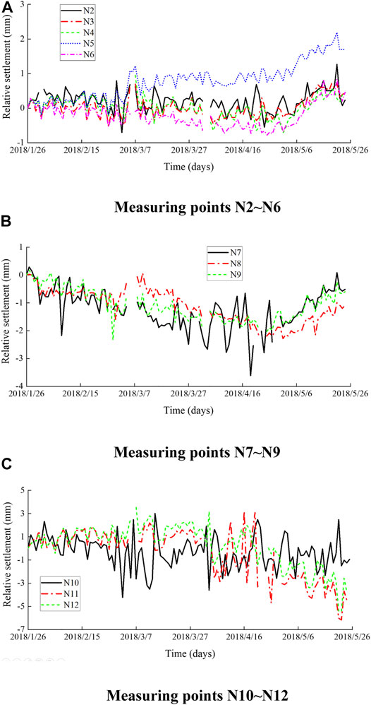
FIGURE 6. Modified relative settlement at the monitoring point of (A) N2 to N6; (B) N7 to N9; and (C) N10 to N12.
According to the field anchor dynamometer and preliminary geological survey results, there is no significant tectonic stress in the field, and the buried depth of the goaf is shallow, so its stability is mainly affected by different lithology, lithology interface, and gravity. Therefore, the initial stress field calculated by the model is constructed according to the self-weight stress of rock mass, and the influence of two kinds of the ore-rock interface is considered, which is shown in Figure 7. The constitutive model used in the model is the mesoscopic elastic creep damage constitutive model, which is referenced by Zhu and Tang, (2004). The model was discretized into 140,057 tetrahedral elements. The representative volume element (RVE) is used in this study to improve computational efficiency. The RVE should be small enough (relative to the macroscopic rock mass) in order to characterize the rock heterogeneity with sufficient precision, but it must be large enough so that it contains enough mesostructural information to be regarded as a material point on a macroscopic scale. According to our previous experience with the numerical simulation at this engineering scale based on the Monte Carlo method, a minimum element size of 0.5 m is selected. The bottom surround boundary of the model is constrained by rollers. In order to avoid the boundary condition influence of the calculation model on the goaf deformation in the calculation process, the boundary sizes of the model are 800 and 600 m, respectively. The degree of surface fluctuation and slope is established by 3Dmine-Rhino, which is achieved by inputting the surface contour elevation data. The results are shown in Figure 7. It can be seen that the interface of different lithology passes through the goaf. The shape of the goaf is determined according to the CMS of the goaf scanning detector. The parameters used in the numerical simulation are shown in Table 1.
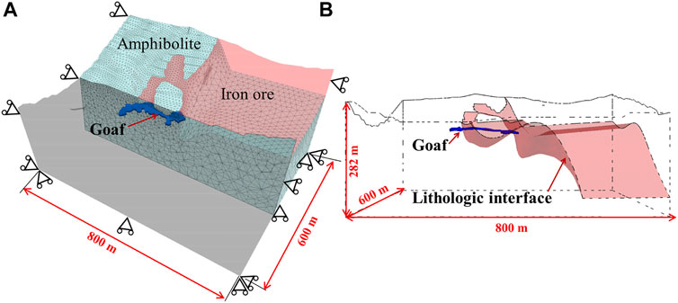
FIGURE 7. Numerical model. (A) Relative position between goaf and model boundary. (B) Relative position of the interface between goaf and lithology.
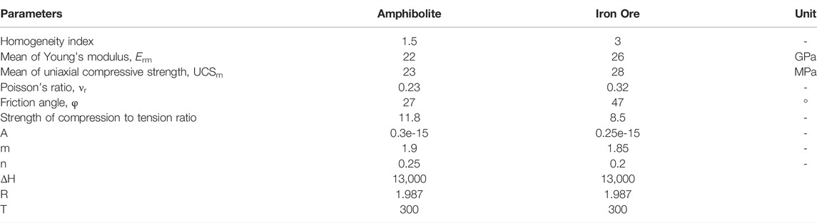
TABLE 1. Parameters used in numerical simulation.
Due to historical reasons, the goaf is formed by irregular mining and disorderly excavation. It is impossible to understand when the excavation is carried out, which means the excavation time is unknown, it brings difficulties to the numerical simulation analysis of the creep damage process of surrounding rock after excavation, and it is difficult to establish the starting point of time-dependent deformation under the influence of excavation. In order to study the current stability of the goaf area, and predict the failure time of the goaf area in the future according to the current stability, the simulation method is established as follows:
(1) Firstly, the creep damage process of roof position A and position B (as shown in Figure 8) after goaf excavation is analyzed by numerical simulation, which obtained the creep deformation time curve of the surrounding rock mass. The mechanical parameters of surrounding rock mass are obtained according to the field investigation, and they are summarized in Table 1. Therefore, the main purpose of this step is to reproduce the creep deformation rate of surrounding rock mass at the present stage by numerical simulation combined with field monitoring, without paying attention to the starting point of creep deformation of surrounding rock mass.
(2) According to the monitoring data of the multipoint displacement meter installed on the site, the deformation rate of the creep deformation of the surrounding rock during the monitoring period (6 June 2018–14 September 2018) was sorted out and analyzed. Then, matching it with the creep deformation curve created by numerical simulation, the period in which they have the same deformation rate will be contrasted.
(3) Then, according to the creep deformation rate verified by the field monitoring, the continuous simulation of the future creep damage process of the surrounding rock is carried out to achieve the stability analysis and deformation prediction of the goaf.
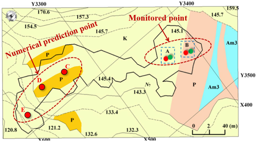
FIGURE 8. Relative position relationship between monitoring points and numerical simulation prediction points in goaf.
The comparison results are shown in Figures 9A, B. It can be seen that the creep deformation rate of the surrounding rock obtained by the numerical simulation and field monitoring is highly consistent in the period of about 20–130 days, indicating that the numerical simulation can well simulate the deformation changing of the goaf roof with time in the field at this stage, and it is able to predict the development of the deformation of the goaf roof in the future and reasonably evaluate the stability of it.
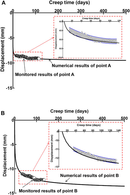
FIGURE 9. Comparison between numerical results and monitored results for (A) point A and (B) point (A).
It can be seen from Figures 9A, B that the creep deformation rate at monitoring point B of goaf roof is larger than that at monitoring point A. The vertical creep deformation of point A is less than 1 mm within 100 days, whilst the point B is less than 2 mm within the same period. The vertical displacement of the two points generally sink to the goaf. The numerical simulation results are in good agreement with the field monitoring results. This shows that the numerical simulation method in this article can simulate and predict the timeliness deformation law of goaf roof at the same time.
Based on the simulation method determined in the above section, the development of roof deformation in the southern goaf is analyzed, and the deformation in the next five years will be simulated and predicted. The simulation results are shown in Figure 10. The period of region I in the figure can be considered as an unknown time-dependent deformation caused by historical reasons. The period of region II is the verification period based on the monitoring data. Area III period is predicted by numerical simulation based on area II period. It can be seen that, at monitoring point C, due to the influence of the lithologic interface, the deformation decreases in the vertical position with the extension of time, which means the point moves slowly to the surface. The deformation rate of monitoring point E is the largest. Compared with the monitoring period, the creep deformation increment could reach over 13 mm in 5 years, which is the position where the deformation of the goaf roof is large. This is consistent with the evolution trend of damage in the goaf area obtained in Figure 11. It can be seen that, under the influence of excavation disturbance, there are small-scale damaged areas on the roof of the southern goaf, but the damaged areas are not connected and scattered. With the development of creep deformation, the damaged areas of the roof of the southern goaf gradually evolve and develop, and local damaged areas appear on the roof and floor of the goaf. When the creep deformation time reaches 5 years, the scattered damaged area of the southern goaf roof forms a connected area, and the damage mode of caving arch is formed at the goaf roof. This shows that the creep deformation in the future is more serious than that in the southern goaf, and the damaged is easier to penetrate to the surface. However, the damaged area in the north of goaf expanded slowly and remained stable.
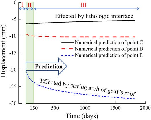
FIGURE 10. Time-dependent deformation of points C, D, and E obtained by numerical modeling.
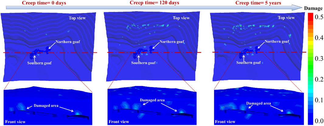
FIGURE 11. Evolution of damaged area of goaf and surrounding rockmass during creep deformation process until 5 years.
In this section, the Mathews stability graph method based on the Hoek–Brown criterion deduced in Section 3.2 is used to evaluate the stability of the southern and the northern goaf in Xiaobeigou. The dip angle of the ore body in this area is 8–25°. The field detection results of the goaf show that the dip angle in the northern goaf is about 7°, and that of the southern goaf is about 5°. Therefore, this calculation is solved according to the near-horizontal orebody, and only the roof stability of the northern and southern goaf is evaluated.
The northern goaf is about 65 m long, 48 m wide, and about 6 m high. The southern goaf is about 130 m in length, 40 m in width, and 5 m in height. According to 3DMine modeling software, the roof contour perimeter and area of the north and south goaf in Xiaobeigou can be obtained, and the hydraulic radius HR of the north and south goaf can be calculated, as shown in Table 2.
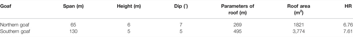
TABLE 2. Hydraulic radius HR of the north and south goaf.
In this article, the structural plane investigation of +145m platform rock mass is carried out by ShapeMetrix3D digital measurement system, and 15 photogrammetry points are selected. The rock mass structural plane is synthesized by the obtained image according to the pixel matching of the same point and the visual distance judgment technology. The average value of the digital measurement results is taken to obtain the information on rock mass joints, cracks, and geometry. The basic rock mass quality index BQ value of the northern goaf is 512.72, whilst the southern goaf is 471.04. According to Eqs 17 and 18, the BQ value can be converted to Barton’ s rock mass quality Q value, and the corresponding Q’ value can be obtained (Liu et al., 2017).
According to the numerical calculation model, the excavation elasticity of the goaf area is calculated, and
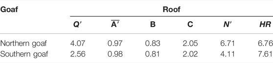
TABLE 3. Calculation of stability number N in each goaf.
Figure 12 shows Mathews stability graph calculation results of the north–south goaf in Xiaobeigou. It can be seen from the figure that the roof of the northern goaf is located in the transition zone, which is a relatively stable state, while the roof of the southern goaf is in the caving zone and has a certain caving risk, which is consistent with the numerical calculation results in Section 5.3. In the calculation process of Mathews stability graph, the rock stress factor

FIGURE 12. Stability graph of Xiaobeigou goaf.
This article takes the goaf area of an open-pit iron mine as the project background, modifying the Mathews stability graph based on its stability evaluation and prediction. It is achieved by applying the combination of fielding monitoring and numerical simulation. The stability of Xiaobeigou shallow goaf in the open-pit iron mine is comprehensively evaluated. The main conclusions are summarized as follows:
1) Based on the Hoek–-Brown criterion with tensile cut-off and considering the spatial stress state, a method for calculating the rock stress factor is proposed. The tensile failure mode is the priority parameter when calculating the stress factor. The stability of shallow goaf in the open-pit iron mine can be evaluated by the proposed piecewise rock stress factor calculation method. The roof of the northern goaf is in the transition zone, and the roof of the southern goaf is in the caving zone.
2) Multipoint displacement meter, anchor force meter, and hydrostatic levelling system are selected as monitoring equipment. During the monitoring period, the maximum stress is 0.61 MPa, the stress value is small, but all of them are in the stress acceleration stage. The displacement of goaf roof presents the characteristics of “deformation period→quiet period→deformation period→quiet period,” but the overall displacement variation is small, which means the roof caving at the incubation period. The relative settlement of the goaf surface is small, fluctuating between −5.4 and 3 mm, in a relatively stable state.
3) The creep damage calculation by using FLAC3D was carried out based on the dynamic feedback of the data measured by the multipoint displacement meter. The 5-year creep calculation result shows that the maximum increment of creep deformation relative to the monitoring period can reach more than 13 mm. The scattered roof damage area in the southern goaf forms a connected domain, and the damage mode of the falling arch is formed at the goaf roof. The expansion speed of the damage area in the northern goaf is relatively slow.
Field monitoring prewarning and numerical simulation both have their unique advantages. The effective combination of the two methods can improve the efficiency of disaster prediction and prewarning to a large extent. Real-time numerical simulation can comprehensively and intuitively demonstrate the mechanical state of deformation and damage in the research area, which provides a more reasonable risk identification. Thses aspects should be further studied and applied to more practical projects.
The original contributions presented in the study are included in the article/Supplementary Material, further inquiries can be directed to the corresponding author.
HJ: conceptualization, methodology, software, and writing, original draft. BY: conceptualization, methodology, software, writing—review and editing, and supervision. KG: review and editing. HOL: software, review and editing. QW: review and editing. YY: investigation. HUL: review and editing.
National Science Foundation of China (Grant nos. U1906208, 51904055, and 51874069), China Postdoctoral Science Foundation (Grant nos. 2021MD703874 and 2021M702015), and Scientific research start-up project of university talent introduction (Grant nos. 2050121006).
Authors HJ, QW, YY and HL were employed by the company Shandong Gold Group Co., Ltd.
The remaining authors declare that the research was conducted in the absence of any commercial or financial relationships that could be construed as a potential conflict of interest.
All claims expressed in this article are solely those of the authors and do not necessarily represent those of their affiliated organizations or those of the publisher, the editors, and the reviewers. Any product that may be evaluated in this article, or claim that may be made by its manufacturer, is not guaranteed or endorsed by the publisher.
Bewick, R. P., and Kaiser, P. K. (2009). “Numerical Assessment of Factor B in Mathews’ Method for Open Stope Design,” in Proceedings of the 3rd CANUS Rock Mechanics Symposium, 11–13.
Chen, G. (1998). Development of High-Order Manifold Method. Int. J. Numer. Methods Eng. 43 (4), 685–712. doi:10.1002/(SICI)1097-0207(19981030)43:4<685::AID-NME442>3.0.CO;2-7
Chen, J., Liu, W., Chen, L., Luo, Y., and Zhong, D. (2020). Failure Mechanisms and Modes of Tunnels in Monoclinic and Soft-Hard Interbedded Rocks: A Case Study. KSCE J. Civil Eng. 24 (4), 4. doi:10.1007/s12205-020-1324-3
Clark, L. M., and Pakalnis, R. C. (1997). “An Empirical Approach for Estimating Unplanned Dilution from Open Stope Hangingwalls and Footwalls,” in Proceedings of 99th Annual General Meeting, Vancouver, B.C, Canada (CIM).
Cui, S., Pei, X., Jiang, Y., Wang, G., Fan, X., Yang, Q., et al. (2021). Liquefaction within a Bedding Fault: Understanding the Initiation and Movement of the Daguangbao Landslide Triggered by the 2008 Wenchuan Earthquake (Ms = 8.0). Eng. Geology. 295, 106455. doi:10.1016/j.enggeo.2021.106455
Dai, Z.-H., You, T., Xu, X., and Zhu, Q.-C. (2018). Removal of Singularities in Hoek-Brown Criterion and its Numerical Implementation and Applications. Int. J. Geomech. 18 (10), 04018127.04018121–04018127.04018119. doi:10.1061/(asce)gm.1943-5622.0001201
Kuscer, D. (1991). Hydrological Regime of the Water Inrush into the Kotredez Coal Mine (Slovenia, Yugoslavia). Mine Water Environ. 10 (1), 93–101. doi:10.1007/BF02914811
Ge, M. (2005). Efficient Mine Microseismic Monitoring. Int. J. Coal Geology. 64 (1/2), 44–56. doi:10.1016/j.coal.2005.03.004
Habibi, R., Moomivand, H., hmadi, M. A., and Asgari, A. (2021). Stability Analysis of Complex Behavior of Salt Cavern Subjected to Cyclic Loading by Laboratory Measurement and Numerical Modeling Using LOCAS (Case Study: Nasrabad Gas Storage Salt Cavern). Environ. Earth Sci. 80 (8), 1–21. doi:10.1007/s12665-021-09620-8
Han, K., Ju, J., Kong, H., Wang, M., Heng, K., and Mengshung, W. (2019). Functional Catastrophe Analysis of Progressive Failures for Deep Tunnel Roof Considering Variable Dilatancy Angle and Detaching Velocity. Rock Mech. Rock Eng. 52 (10), 3987–3997. doi:10.1007/s00603-019-01808-6
He, M. C., Miao, J. L., and Feng, J. L. (2010). Rock Burst Process of limestone and its Acoustic Emission Characteristics under True-Triaxial Unloading Conditions. Int. J. Rock Mech. Mining Sci. 47 (2), 286–298. doi:10.1016/j.ijrmms.2009.09.003
He, Y., and Kusiak, A. (2017). Performance Assessment of Wind Turbines: Data-Derived Quantitative Metrics. IEEE Trans. Sustain. Energ. 9 (1), 65–73. doi:10.1109/TSTE.2017.2715061
Hoek, E., and Carranza-Torres, C. (2002) Hoek-Brown Failure Criterion—2002 Edition. In: Proceedings of the Fifth North American Rock Mechanics Symposium, 267–273.
Jia, H., Cheng, G., Li, J., Liu, H., and Qian, J. (2021). A Correction Method for the Ambient Temperature-Induced Error in Hydrostatic Leveling Systems and Application. Measurement. 172, 10880. doi:10.1016/j.measurement.2020.108880
Jia, H., Guan, K., Zhu, W., Liu, H., and Liu, X. (2020). Modification of Rock Stress Factor in the Stability Graph Method: a Case Study at the Alhada Lead-Zinc Mine in Inner Mongolia, China. Bull. Eng. Geol. Environ. 79 (6), 3257–3269. doi:10.1007/s10064-020-01753-7
Jiang, Q., Su, G., Feng, X. T., Chen, G., Zhang, M. Z., and Liu, C. (2019). Excavation Optimization and Stability Analysis for Large Underground Caverns under High Geostress: A Case Study of the Chinese Laxiwa Project. Rock Mech. Rock Eng. 52 (1), 895–915. doi:10.1007/s00603-018-1605-z
Li, H., Deng, J., Feng, P., Pu, C., Arachchige, D. D. K., and Cheng, Q. (2021a). Short-Term Nacelle Orientation Forecasting Using Bilinear Transformation and ICEEMDAN Framework. Front. Energ. Res. 9, 780928. doi:10.3389/fenrg.2021.780928
Li, H., Deng, J., Yuan, S., Feng, P., and Arachchige, D. D. K. (2021b). Monitoring and Identifying Wind Turbine Generator Bearing Faults Using Deep Belief Network and EWMA Control Charts. Front. Energ. Res. 9, 799039. doi:10.3389/fenrg.2021.799039
Li, H., He, Y., Xu, Q., Deng, j., Li, W., and Wei, Y. (2022). Detection and Segmentation of Loess Landslides via Satellite Images: a Two-phase Framework. Landslides. 19, 673–686. doi:10.1007/s10346-021-01789-0
Liu, Q., Liu, J., Pan, Y., Kong, X., and Hong, K. (2017). A Case Study of Tbm Performance Prediction Using a Chinese Rock Mass Classification System – Hydropower Classification (Hc) Method. Tunnelling Underground Space Tech. 65, 140–154. doi:10.1016/j.tust.2017.03.002
Majdi, A., and Beiki, M. (2010). Evolving Neural Network Using a Genetic Algorithm for Predicting the Deformation Modulus of Rock Masses. Int. J. Rock Mech. Mining Sci. 47 (2), 246–253. doi:10.1016/j.ijrmms.2009.09.011
Mathews, K. E., Hoek, E., and Wyllie, D. C. (1981). Prediction of Stable Excavations for Mining at Depths below 1000 Metres in Hard rockCANMET Report. Vancouver, Canada: Mines& Resources.
Mawdesley, C., Trueman, R., and Whiten, W. J. (2001). Extending the Mathews Stability Graph for Open-Stope Design. Mining Tech. 110 (1), 27–39. doi:10.1179/mnt.2001.110.1.27
Mawdesley, C. (2004). Using Logistic Regression to Investigate and Improve an Empirical Design Method. Int. J. Rock Mech. Mining Sci. 41 (3), 507–508. doi:10.1016/j.ijrmms.2003.12.039
Mitri, H. S., Hughes, R., and Zhang, Y. (2011). New Rock Stress Factor for the Stability Graph Method. Int. J. Rock Mech. Mining Sci. 48 (1), 141–145. doi:10.1016/j.ijrmms.2010.09.015
Müller, W. (1991). Numerical Simulation of Rock Bursts. Mining Sci. Tech. 12 (1), 27–42. doi:10.1016/0167-9031(91)91513-H
Nickson, S. D. (1992). Cable Support Guidelines for Underground Hard Rock Mine Operations. Vancouver: University of British Columbia.
Nomikos, P. P., Sofianos, A. I., and Tsoutrelis, C. E. (2002). Structural Response of Vertically Multi-Jointed Roof Rock Beams. Int. J. Rock Mech. Mining Sci. 39 (1), 79–94. doi:10.1016/s1365-1609(02)00019-9
Ohnishi, Y., Sasaki, T., Koyama, T., Hagiwara, I., Miki, S., and Shimauchi, T. (2014). Recent Insights into Analytical Precision and Modelling of DDA and NMM for Practical Problems. Geomechanics and Geoengineering. 9 (2), 97–112. doi:10.1080/17486025.2013.871066
Potvin, Y. (1988). Empirical Open Stope Design in Canada. Vancouver: University of British Columbia.
Qiao, C., Guo, Y. H., and Li, C. H. (2021). Study on Rock Burst Prediction of Deep Buried Tunnel Based on Cusp Catastrophe Theory. Geotechnical Geol. Eng. 39 (1), 1–15. doi:10.1007/s10706-020-01547-4
Rouabhi, A., Tijani, M., Moser, P., and Goetz, D. (2005). Continuum Modelling of Dynamic Behaviour and Fragmentation of Quasi-Brittle Materials: Application to Rock Fragmentation by Blasting. Int. J. Numer. Anal. Meth. Geomech. 29 (7), 729–749. doi:10.1002/nag.436
Shi, G. H. (1988). Discontinuous Deformation Analysis: A New Numerical Model for the Statics and Dynamics of Block System. Berkeley: Department of Civil Engineering, University of California.
Sidorenko, M., Orlov, D., Ebadi, M., and Koroteev, D. (2021). Deep Learning in Denoising of Micro-computed Tomography Images of Rock Samples. Comput. Geosciences. 151 (2), 104716. doi:10.1016/j.cageo.2021.104716
Stewart, P. C., and Trueman, R. (2001). “The Extended mathews Stability Graph: Quantifying Case History Requirements and Site-specific Effects,” in Proceedings of International Symposium on Mining Techniques, Chicago, 1-4, Oct. 2001 (CIM), 84–92.
Sun, X., Zhao, C., Tao, Z., Kang, H., and He, M. (2021). Failure Mechanism and Control Technology of Large Deformation for Muzhailing Tunnel in Stratified Rock Masses. Bull. Eng. Geol. Environ. 80 (6), 4731–4750. doi:10.1007/s10064-021-02222-5
Suorineni, F. T. (1998). Effects of Faults and Stress on Open Stope Design. Canada: Waterloo:University of Waterloo.
Suorineni, F. T. (2010). The Stability Graph after Three Decades in Use: Experiences and the Way Forward. Int. J. Mining, Reclamation Environ. 24 (4), 307–339. doi:10.1080/17480930.2010.501957
Tang, C., Wang, J., and Zhang, J. (2010). Preliminary Engineering Application of Microseismic Monitoring Technique to Rockburst Prediction in Tunneling of Jinping II Project. J. Rock Mech. Geotechnical Eng 2 (3), 193–208. doi:10.3724/SP.J.1235.2010.00193
Tang, J., Dai, Z., Wang, Y., and Zhang, L. (2019). Fracture Failure of Consequent Bedding Rock Slopes after Underground Mining in Mountainous Area. Rock Mech. Rock Eng. 52 (8), 2853–2870. doi:10.1007/s00603-019-01876-8
Vallejos, J, Delonca, A., and Perez, E. (2018). Three-dimensional Effect of Stresses in Open Stope Mine Design. Int. J. Mining, Reclamation Environ. 32 (5), 355–374. doi:10.1080/17480930.2017.1309833
Wang, J. X., Tang, S. B., Heap, M. J., Tang, C. A., and Tang, L. X. (2021). An Auto-Detection Network to Provide an Automated Real-Time Early Warning of Rock Engineering Hazards Using Microseismic Monitoring. Int. J. Rock Mech. Mining Sci. 140 (21), 104685. doi:10.1016/j.ijrmms.2021.104685
Wang, X., Guan, K., Yang, T., and Liu, X. (2021). Instability Mechanism of Pillar Burst in Asymmetric Mining Based on Cusp Catastrophe Model. Rock Mech. Rock Eng. 54 (3), 1463–1479. doi:10.1007/s00603-020-02313-x
Xia, K., Chen, C., Zhou, Y., Liu, X., Zheng, Y., and Pan, Y. (2019). Catastrophe Instability Mechanism of the Pillar-Roof System in Gypsum Mines Due to the Influence of Relative Humidity. Int. J. Geomechanics. 19 (4), 1–16. doi:10.1061/(asce)gm.1943-5622.0001378
Xsa, B., Cza, B., Yong, Z., Feng, C. C., Sza, B., and Kz, B. (2021). Physical Model Test and Numerical Simulation on the Failure Mechanism of the Roadway in Layered Soft Rocks. Int. J. Mining Sci. Tech 31 (2), 291–302. doi:10.1016/j.ijmst.2021.01.003
Yang, W., Jiang, Y., Gu, X., Wang, Z., Shang, Y., and Zeng, W. (2021). Deformation Mechanism and Mechanical Behavior of Tunnel within Contact Zone: A Case Study. Bull. Eng. Geology. Environ. 80 (7), 5657–5673. doi:10.1007/s10064-021-02255-w
Yi, S. A., Xc, A., and Jw, B. (2021). Distributed Fibre Optic Monitoring of Damaged Lining in Double-Arch Tunnel and Analysis of its Deformation Mode. Tunnelling Underground Space Tech. 110, 103812. doi:10.1016/j.tust.2021.103812
Zhang, J., Zhang, Q., Sun, Q., Gao, R., Germain, D., and Abro, S. (2015). Surface Subsidence Control Theory and Application to Backfill Coal Mining Technology. Environ. Earth Sci. 74 (2), 1439–1448. doi:10.1007/s12665-015-4133-0
Zhang, K., Xue, Y., Xu, Z., Su, M., and Li, Z. (2021). Numerical Study of Water Inflow into Tunnels in Stratified Rock Masses With a Dual Permeability Model. Environ. Earth Sci. 80 (260), 1–12. doi:10.1007/s12665-021-09550-5
Zhou, J., Wei, J., Yang, T., Zhang, P., Liu, F., and Chen, J. (2021). Seepage Channel Development in the crown Pillar: Insights from Induced Microseismicity. Int. J. Rock Mech. Mining Sci. 145, 104851. doi:10.1016/j.ijrmms.2021.104851
Zhu, W. C., and Tang, C. A. (2004). Micromechanical Model for Simulating the Fracture Process of Rock. Rock Mech. Rock Eng. 37 (1), 25–56. doi:10.1007/s00603-003-0014-z
Keywords: Mathews stability graph, field monitoring, numerical simulation, creep damage, goaf stability
Citation: Jia H, Yan B, Guan K, Liu H, Wu Q, Yin Y and Liu H (2022) Stability Analysis of Shallow Goaf Based on Field Monitoring and Numerical Simulation: A Case Study at an Open-Pit Iron Mine, China. Front. Earth Sci. 10:897779. doi: 10.3389/feart.2022.897779
Received: 16 March 2022; Accepted: 04 April 2022;
Published: 09 May 2022.
Edited by:
Yusen He, Grinnell College, United StatesReviewed by:
Lu Jun, Shenzhen University, ChinaCopyright © 2022 Jia, Yan, Guan, Liu, Wu, Yin and Liu. This is an open-access article distributed under the terms of the Creative Commons Attribution License (CC BY). The use, distribution or reproduction in other forums is permitted, provided the original author(s) and the copyright owner(s) are credited and that the original publication in this journal is cited, in accordance with accepted academic practice. No use, distribution or reproduction is permitted which does not comply with these terms.
*Correspondence: Baoxu Yan, eWFuYmFveHVAeHVzdC5lZHUuY24=
Disclaimer: All claims expressed in this article are solely those of the authors and do not necessarily represent those of their affiliated organizations, or those of the publisher, the editors and the reviewers. Any product that may be evaluated in this article or claim that may be made by its manufacturer is not guaranteed or endorsed by the publisher.
Research integrity at Frontiers
Learn more about the work of our research integrity team to safeguard the quality of each article we publish.