High-precision downward continuation of the potential field based on the D-Unet network

Potential field data are of great significance to the study of geological characteristics. Downward continuation of the potential field converts potential field data from a high plane to a low plane. Since this method is mathematically an inverse problem solution, it is unstable. The Tikhonov regularization strategy is an effective means of the downward continuation of the potential field. However, achieving high-precision requirements in the stage of precise geophysical exploration is still challenging. Deep learning can effectively solve unstable problems with excellent nonlinear mapping capabilities. Inspired by this, for the downward continuation of the potential field, we propose a new neural network architecture for downward continuation named D-Unet. This study uses the potential field data of a high horizontal plane and the initial model as the network’s input, with the corresponding low-level data serving as the output for supervised learning. Moreover, we add noise to 10% of the data in the training dataset. Model testing shows that our D-Unet has higher accuracy, validity, and stability. In addition, adding noise to the training data can further improve the robustness of the model. Finally, we use the actual potential data of a particular place in northeast China to test our model and satisfactory results have been obtained.

1 Introduction

Downward continuation of a potential field is an effective means to improve the accuracy of data interpretation, which plays an essential role in the crustal structure (Lou, 2001; Zhang et al., 2013a), construction of a geomagnetic navigation database (Xu, 2007; Zeng et al., 2009; Wang and Tian, 2010), geological structure identification (Liu, 2008), and disaster prevention. Downward continuation of the potential field is a method to convert potential field data from a high horizontal plane to a low one, making the potential field data closer to the field source and increasing geological interpretation resolution (Zeng et al., 2011a; Wang et al., 2012). At the same time, it is also the core algorithm for potential field data processing, inversion, or other subsequent steps. The process of potential field downward continuation is mathematically an ill-posed problem. It can be concluded as the solution of the first Fredholm integral equation (Yang, 1997; Wang, 2007). Therefore, its accuracy, stability, and effectiveness have become the focus of extensive research by many scholars (Zhang, 2013).

Since Bateman (1946) and Peters (1949) used the Taylor series method to carry out the downward continuation of the potential field in the 1940s, many scholars have researched these problems. Research in this problem can be divided into two categories: spatial domain and wave-number domain methods. The first one has high accuracy, but there are some disadvantages (e.g., complex calculation formula, complicated process, and low efficiency). Also, it is unsuitable for many quantity calculations because of its poor practicability (Zeng et al., 2013). The spatial domain calculation methods mainly include the boundary element method (Liu et al., 1990; Xu et al., 2004), equivalent source method (Dampney, 1969; Syberg, 1972; Emilia, 1973; Hou et al., 1984; Hou et al., 1985; Xia et al., 1993; Xu et al., 2004; Liu et al., 2007; Hunag et al., 2009), and integral iterative method (Xu, 2006; Xu, 2007). Among these, the equivalent source method is one of the most extensive continuation methods. Its main shortcoming lies in that the calculation accuracy is related to the distribution of the equivalent field source, and the calculation is time-consuming (Bhattacharyya and Chan, 1977; Ivan, 1994; Zhang, 2013). The integral iterative method has a tremendous effect, achieving an extended depth of 20 times the point distance or even more significantly (Xu, 2006). Despite the excellent effect and strong convergence (Zhang et al., 2009), it also has problems such as noise amplification (Zeng et al., 2011b). The Fast Fourier Transform method (FFT) has the advantages of high computational efficiency and suitability for many quantity calculations. However, the calculation process will magnify the high-frequency noise, resulting in the limited accuracy of the frequency domain method (Zeng et al., 2011a). Therefore, many scholars have reformed downward continuation operators, including the Wiener filtering method (Clarke, 1969; Pawlowski, 1995; Zeng et al., 2014), optimization filtering method (Guo et al., 2012), regularization method (Luan, 1983; Liang, 1989; Ivan, 1994; Ma et al., 2013; Zeng et al., 2013), and derivative and compensation method (Mao and Wu, 1998; Cooper, 2004). The Wiener filtering method has a small continuation depth and is affected by the potential field’s noise and power spectrum ratio (Zeng et al., 2014). The regularization method is a potential field downward continuation method widely used nowadays, including the Tikhonov regularization and Landweber regularization methods. However, its down progression process also has the disadvantages of poor stability, low continuation depth, and high parameter sensitivity (Zhang, 2013). Most scholars only focus on solving the continuation process by using mathematical methods. Vaníček et al. (2017) proposed that it is meaningless to seek an accurate solution under the influence of noise due to the unique nature of downward continuation calculations and to preferably regard the problem as the optimal estimation of statistical problems.

With the rapid development of computer technology, computing ability is greatly improved. New solutions for downward continuation may exist, such as deep learning (DL). DL is a thinking mode that simulates the mechanism of the human brain. Based on the sample dataset, the multi-level network structure model is trained to analyze and calculate the sample data outside the scene (Yin et al., 2015). Composed of multiple layers of single neurons, DL transmits parameters back and changes the weight of connections to obtain powerful nonlinear mapping ability after several training rounds (Lecun et al., 2015). Hinton and Salakhutdinov (2006)proposed that the multi-layer neural network has a significant learning ability of features and can achieve network optimization through pre-training, which led to DL’s blossoming. DL has made achievements in various fields, especially in medical imaging (Li et al., 2018), semantic image segmentation (Krizhevsky et al., 2012), machine translation (Bahdanau et al., 2014; Sutskever et al., 2014), speech recognition (Dahl et al., 2011; Hinton G. et al., 2012), extensive data analysis (Sun et al., 2014), and other fields. Due to the aforementioned characteristics and advantages, DL has been increasingly widely applied in geophysics (Wang et al., 2020). The main contents of DL include seismic data interpretation and processing (Xi and Huang, 2018; Li et al., 2019), magnetotellurics inversion (Puzyrev, 2019), gravity and magnetic inversion (Zhang et al., 2021), and data noise elimination (Han et al., 2018; Li et al., 2020; Tian et al., 2020), and all obtained satisfactory results.

Based on this, we try to introduce the DL method into the downward continuation of the potential field to improve the solution accuracy of the ill-posed continuation of the potential field by using DL’s more efficient mapping ability. This study first generates a random-like anomalous body model by the layered point-throwing method. The forward modeling results are used as the output of the DL network. The high plane potential field theory data are generated by the upward continuation of the potential field as the network’s input. At the same time, the wave-number domain iterative Tikhonov regularization method (Zeng et al., 2013) was used for downward continuation results of high-plane potential field data as the initial model and input of the network to form a joint drive. The aforementioned three parts of data were combined into sample data pairs, and 10% of the sample data were randomly selected for adding noise. Then, based on Densenet, nested Unet, the network structure is constructed to form the DL network model of downward continuation in this study, which is called D-Unet. Then the proposed method is tested by theoretical and practical data to verify its accuracy, effectiveness, and stability.

2 Methodology of dataset construction and the DL network

2.1 Downward continuation of the original dataset construction

Since the theory is the same as the method in the downward continuation of gravity and magnetic potential field data, the difference only lies in the physical property and information carrier. The gravity field is temporarily selected as the calculation carrier for constructing the original dataset of downward continuation of the potential field in this study. At the same time, the innovation of the downward continuation method of the potential field not only works on the horizontal plane but also on curved surface data. However, our work in this study did not cover the curve surface data. This content can be studied in more depth later.

2.1.1 Low horizontal plane theory data generation

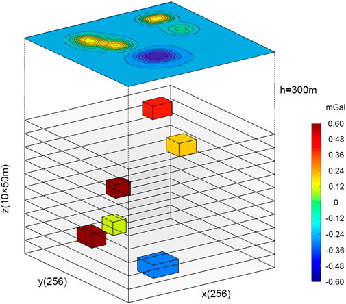
Yu (2009) proposed using potential field separation cutting and downward continuation to obtain underground anomalies caused by sources at different depths, including the surface and the top of deep layers. The inversion operation of the anomaly can determine the physical properties and conditions of geological bodies at different depths. Using this method for reference, we first divide layers at different depths into lattice points. Layers at different depths are cut into prismatic aggregates of equal size and different physical properties, called stratification. Then, on each layer of prism assembly, different rectangular prisms are randomly selected for differential residual density assignment to simulate the abnormal body with different conditions, the casting point. Then the overall potential field data observed in the low plane can be simulated by the forward calculation of the rectangular prism in each layer and related mathematical processing. This method is the theoretical basis for generating original potential field data by the hierarchical point casting method.

Since the research focus of this study is to improve the accuracy of downward continuation by using deep learning methods, a fast, stable, and large-scale model forward algorithm is urgently needed to construct sufficient sample datasets of potential field downward continuation required for typical deep learning model training. In this study, the frequency domain forward method provided by Yu (2009) is used to generate many datasets. Compared with the forward modeling method in the space domain, the frequency domain is characterized by fast forward modeling and a simplified formula, which meets the requirements of this study. The process is as follows.

Assume that the center coordinates of each small rectangular prism are $\left(x_{\mathit{0}j},y_{\mathit{0}j}\right)$. The assigned residual density is ${\rho }_j,\mathrm{j}=\left(\mathrm{1,2},\dots ,MN\right)$. The embedding depth between the top surface of the prism and the observation surface is $dh$. $MN$ means to divide the layer into $M\times N$ prisms. The following is a formula for calculating the spectrum ${\stackrel{\sim }{u}}_j\left(k_x,k_y\right)$ of the gravity anomalies $u_j\left(x,y\right)$ generated by a single prism at the observation plane $\left(x,y\right)$ :

${\stackrel{\sim }{u}}_j\left(k_x,k_y\right)=2\pi G{\rho }_j\bullet \frac{4}{k_x{k}_y}\sin \left(\frac{l{k}_x}{2}\right)\bullet \sin \left(\frac{b{k}_y}{2}\right)\bullet \frac{e^{-h\bullet \omega }}{\omega }\left(1-e^{-dh\omega }\right)\bullet e^{-i\left(k_x\bullet x_{0j}+k_y\bullet y_{0j}\right)}.(1)$

The following is a formula for calculating the spectrum $\stackrel{\sim }{u}\left(k_x,k_y\right)$ of the gravity anomalies $u\left(x,y\right)$ generated by a single prism at the observation plane $\left(x,y\right)$ in the whole depth layer:

$\stackrel{\sim }{u}\left(k_x,k_y\right)=2\pi G\bullet \frac{4}{k_x{k}_y}\sin \left(\frac{l{k}_x}{2}\right)\bullet \sin \left(\frac{b{k}_y}{2}\right)\bullet \frac{e^{-h\bullet \omega }}{\omega }\left(1-e^{-dh\omega }\right){\displaystyle \sum }_{j=1}^{MN}{{\rho }_{j}e}^{-i\left(k_x\bullet x_{0j}+k_y\bullet y_{0j}\right)},(2)$

where $k_x$ and $k_y$ are wave numbers in $x$ and $y$ directions. $G$ is the universal gravitational constant. $\omega =\sqrt{k_x^2+k_y^2}$ is the angular frequency.

The final monolayer gravity anomaly result $u\left(x,y\right)$ is obtained by inverse Fourier transform of $\stackrel{\sim }{u}\left(k_x,k_y\right)$.

To better simulate the measured potential field data under natural working conditions and avoid the subsequent long-distance continuation distortion due to the small selection range of the measured area, the area is expanded to $256\times 256$ prisms in this study. Each prism is $50m$ in length, width, and height, thus, forming a layer source with a single depth. The depth of the top surface of all source layers is selected in the range of $300-800m$ below the observation plane. The height of the single layer and prism is $50m$, with 10 layers in total. The residual density of a single prism in each layer was randomly assigned with a range of $\left[-0.6,0.6\right]\left(g/{cm}^3\right)$ to form the original anomalous body distribution. The position diagram of the layered projection prism is shown in Figure 1.

FIGURE 1

FIGURE 1. Position diagram of the layered projection prism.

The prism of each depth layer is substituted into Eqs 1, 2 for calculation, and then the inverse Fourier transform is performed to obtain the monolayer gravity anomaly results. After all the depth layers in the $300-800m$ interval below the observation surface are completely calculated, all their contents are superimposed to obtain the final single potential field data on the observation surface.

2.1.2 Calculation of the potential field at the high horizontal plane

This study extends the low plane potential field data in the frequency domain to obtain the high plane potential field data. Through this step, the gravity and magnetic potential field data obtained from the airborne geophysical survey can be simulated, providing primary sample data for subsequent calculation and model training.

The upward continuation of the potential field is relatively stable (Xu, 2006; Zeng et al., 2011a; Xiong, 2016). The main methods include the wave-number domain and spatial domain. The wave-number domain includes FFT methods and sampling grouping, which are simple, fast, and suitable for large-scale model calculation. Therefore, in constructing the high plane potential field theory dataset in this study, we use the FFT method to carry out the upward continuation to obtain specific and sufficient sample data.

Many pieces of potential field data at the observation plane$\left(z=0\right)$ are generated through the steps in Section 2.1.1. $u\left(x,y,0\right)$ represents the potential field at the height $z=0$. The potential field data are converted from the spatial domain to the wave-number domain through the FFT method, as expressed in Eq. 3.

$\stackrel{\sim }{u}\left(k_x,k_y,0\right)=F\left[u\left(x,y,0\right)\right],(3)$

where $F\left[u\left(x,y,0\right)\right]$ is expressed as the Fast Fourier Transform of $u\left(x,y,0\right)$. We introduce an upward continuation operator: $\phi \left(\omega \right)=e^{-\omega \mathrm{h}}$. The $h\left(h>0\right)$ is the height of upward continuation, which means that the potential field is continued upward to the plane $z=0$. Inverse FFT is performed on the generated potential field data in the wave-number domain, which is the upward continuation formula, Eq. 4:

$u\left(x,y,h\right)=F^{-1}\left[\phi \left(\omega \right)\bullet \stackrel{\sim }{u}\left(k_x,k_y,0\right)\right].(4)$

$F^{-1}$ is the inverse Fourier transform. The formula is proven to be very stable. (Xu, 2007)

Qiu et al. (2017) proposed that the Gibbs effect is a possible potential field based on frequency domain upward continuation. There will be leakage problems such as frequency, high-frequency confusion, and boundary effect. Thus, it leads to a calculated value to produce the phenomenon of deviation. Therefore, we effectively use Zhang et al.’s (2013b) proposed continuation method in wave-number domain transformation in the spatial domain. The Gibbs effect in the continuation process is reduced and the continuation accuracy is improved.

2.1.3 Initial model construction

The Tikhonov method was used to construct the initial model. The Tikhonov regularization method provides a new downward continuation operator, which attempts to improve its low-pass filtering ability, adaptability, and stability by suppressing its high-pass characteristics and filtering high-frequency interference (An and Guan, 1985). Zeng et al. (2011a) pointed out that the Tikhonov regularization method has a saturation effect. The error estimation between the solution obtained by the Tikhonov regularization method and the theoretical solution cannot achieve order optimization, so there is room for improvement.

The time problem of calculating is one of the reasons why we use the Tikhonov method. The spatial domain method trades computation time for accuracy. However, most researchers and we do not have high computing power and we do not have enough time. Additionally, a dataset consisting of a large number of samples is much more necessary for DL. It provides the target and preliminary information for model training and indicates the characteristic direction domain, which can significantly improve the rapid convergence ability of model training while saving time and computation power. Thus, as the main content of this study is to improve the accuracy of the downward continuation of the potential field through deep learning, Tikhonov’s downward continuation part can be used and it is not the final result.

We can use Eq. 5, which is the transformation of Eq. 4, to compute the downward continuation:

$u\left(x,y,h\right)=F^{-1}\left[{\phi }^{-1}\left(\omega \right)\bullet \stackrel{\sim }{u}\left(k_x,k_y,0\right)\right].(5)$

The downward continuation operator is ${\phi }^{-1}\left(\omega \right)$. The downward continuation operator increases exponentially with the increase in $\omega$. Because of this, the original downward continuation operator amplifies the noise infinitely for possible high-frequency noise. Therefore, this method has poor stability and is unsuitable for our study. Zeng et al. (2011a) deduced the operator in the wave-number domain corresponding to Tikhonov regularization, and the calculation formula of the operator is as follows:

$\Phi \left(\omega \right)=\frac{\phi \left(\omega \right)}{{\phi }^2\left(\omega \right)+\alpha }.(6)$

$\alpha$ is the regularization parameter used to improve the stability and smoothness of the continuation process. In this study, empirical data $\alpha$ were set to 0.01 (Tikhonov et al., 1977; Liang, 1989; Chen and Xiao, 2007). First, the potential field data are converted from the spatial domain to the wave-number domain by Eq. 3. Then, the downward continuation operator ${\phi }^{-1}\left(\omega \right)$ in Eq. 5 is replaced by the Tikhonov regularization downward continuation operator (Eq. 6). The final continuation formula Eq. 7 is obtained as follows:

$u\left(x,y,h\right)=F^{-1}\left[\Phi \left(\omega \right)\bullet \stackrel{\sim }{u}\left(k_x,k_y,0\right)\right].(7)$

2.1.4 Construction of the data sample and add-noise sample

The three parts of the dataset formed from Sections 2.1.1–2.1.3 are combined to form the theoretical training dataset. We use the numerical model of synthetic data of 2,000 sample data. Owing to this article’s sample data for simulation data, there are some differences between the actual data. To further improve the calculation scene of generality, we randomly choose 10% theory samples, adding 5% random noise to enhance the convergence ability and robustness of the model.

2.2 D-Unet neural network architecture

2.2.1 Introduction to D-Unet network architecture

Among deep learning methods, Unet and Densenet are two excellent network structures. As an improved structure of the full convolutional neural network (FCN) (Long et al., 2015), the Unet adopts a completely symmetrical “U”-type coding–decoding structure to extract sample data features through downsampling and fusion, splicing channel numbers, and improving the effectiveness and generalization ability of information (Ronneberger et al., 2015). However, due to the operation mode of the Unet, the overlapping part of the neighborhood will be repeatedly calculated so that when the network layer is deep, the model occupies a large amount of GPU memory and the computing speed is too slow (Li et al., 2018). If the parameters are not correctly selected, there may be a gradient explosion or gradient disappearance (Tong et al., 2020). Given these problems, we try to replace the downsampling part of the Unet network with the Densenet network structure to form a new network structure named D-Unet. Densenet (Huang et al., 2017) can effectively alleviate the gradient disappearance problem of the model. At the same time, in the case of using fewer parameters, feature repetition is used to strengthen feature transfer and reduce feature loss. Therefore, we can use small samples for training and solving complex problems.

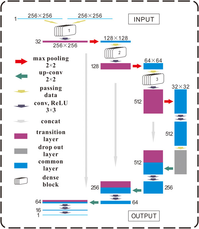
The model-building method in this study is to extract the backbone of the Unet network structure, i.e., the backbone of the “U-shaped” coding–decoding structure, and then extract and process some network structure features in Densenet to form a dense block to replace the feature extraction part of “U-shaped” structure in the Unet network. Thus, the final D-Unet network structure is formed. Figure 2 is the logical diagram of the D-Unet network architecture used in this study.

FIGURE 2

FIGURE 2. Logical diagram of the D-Unet network architecture.

2.2.2 Unet backbone network structure

The Unet network proposed by Ronneberger et al. (2015), a deep learning network structure, is applied for image segmentation in the biomedical field, which solved the problem of improving the segmentation accuracy of the model in the case of a small sample dataset. The backbone part of the network structure mainly includes the convolution layer, pooling layer, upsampling layer, dropout layer, and other parts. The details of each part are described as follows.

2.2.2.1 Convolution layer

The convolution layer is the core operation and Unet deep learning network component. Its original intention is convolution operation in the mathematical sense, which evolved into a feature extraction operation in a neural network by adding a series of computer language modifications and restriction rules. The convolution layer consists of elements constantly modified by extracting image features. The main parameters of the convolution layer include filter, stride, and pad. The function of the receptive field is to limit the range size of single feature extraction and extract features dynamically according to the modified size. The larger the receptive field is, the more complex features can be extracted. The deeper the network is, the larger the receptive field will be. The role of step size is to determine the position distance of the receptive field sweeping the adjacent area. The pad’s function is to fill the feature map with different methods to retain adequate edge information to the maximum extent when the feature map is formed after receptive field scanning.

The input and output dimensions’ calculation formula (Eq. 8) of the convolution layer is as follows:

$n=\left[\frac{m+2p-f}{s}+1\right],(8)$

where $m$ is the input size $\left(m\times m\right)$, $n$ is the output size $\left(n\times n\right)$, $f$ is the filter size $\left(f\times f\right)$, $s$is the stride, and $p$ is the number of pixels of the pad.

In the convolution layer operation, we need to introduce an activation function to improve the network’s nonlinear mapping and generalization ability, which plays a vital role. Commonly used activation functions include ReLU, Sigmoid, and Tanh functions, which are expressed as follows (Eqs 9, 10, 11):

$f_{ReLU}\left(x\right)=\max 0,x),(9)$

$f_{sigmoid}\left(x\right)=\frac{1}{1+e^{-x}},(10)$

$f_{\mathit{Tanh}}\left(x\right)=\frac{e^{2x}-1}{e^{2x}+1.}(11)$

The ReLU function is an excellent activation function for deep learning due to its unique properties (e.g., fast convergence, weak gradient disappearance, and sparse expression). Therefore, all the activation functions used in this study are ReLU functions.

2.2.2.2 Pooling layer

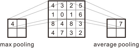
The primary function of the convolution layer is feature extraction, but due to the pad, the effect of the convolution layer on the dimension of the feature image is not apparent. However, the high dimension of feature images has significant disadvantages in neural network training, which will increase the training time and quickly lead to problems such as overfitting the model. Therefore, the pooling step, also called down-sampling, is introduced in the Unet to reduce the dimension of the original feature image according to the size of the pooling window, and a value is used to replace the value of the window size area. There are mainly two pooling methods for the pooling layer: maximum pooling and mean pooling. Using the maximum value to replace it is called maximum pooling, and using the range means to replace it is called mean pooling. The function of the pooling layer is evident, including reducing dimensions to improve operation speed and preventing model overfitting from improving robustness. There is a diagram of the pooling method in Figure 3.

FIGURE 3

FIGURE 3. Diagram of the pooling method.

Maximum pooling is a nonlinear operation process. In contrast, mean pooling is a linear operation process. We use the maximum pooling method more in this model to improve the model’s generalization ability.

2.2.2.3 Dropout layer

Hinton G. E. et al. (2012) proposed the concept of the dropout layer, which aims to prevent the fitting phenomenon in the training process of large models and improve the generalization ability of models. The operation logic of the dropout layer is to set the probability of discarding so that the activation value of probability P neurons is changed to zero randomly during the operation of this step in model training. The neuron is hidden to prevent features’ complex reuse and synergy and weaken the intricate connection between neurons. This method efficiently improves the model’s generalization ability and has a noticeable effect.

2.2.2.4 Upsampling layer

After the operation between the previous layers, the model’s features are fully extracted and the resolution is the lowest. The ultimate purpose of setting up the model is to use the continuation of the position field, which can be approximately regarded as an image-like processing method. The input and output are values of the same dimension (pixel values in image processing). Therefore, the resolution needs to be raised to the same dimension as the input data after the previous steps. At this point, the upper sampling layer is needed to assist.

The upper sampling layer can be understood as the reverse process of the lower sampling layer, and its function is to enlarge the dimension of the data (the image domain is to improve the image’s resolution). The main upsampling methods include linear interpolation, inverse pooling, and deconvolution. In deconvolution operation, the model will also conduct secondary learning, which better affects the continuation and reduction of features. Therefore, the upsampling methods adopted in this study are all deconvolution methods.

2.2.3 Dense block model training module

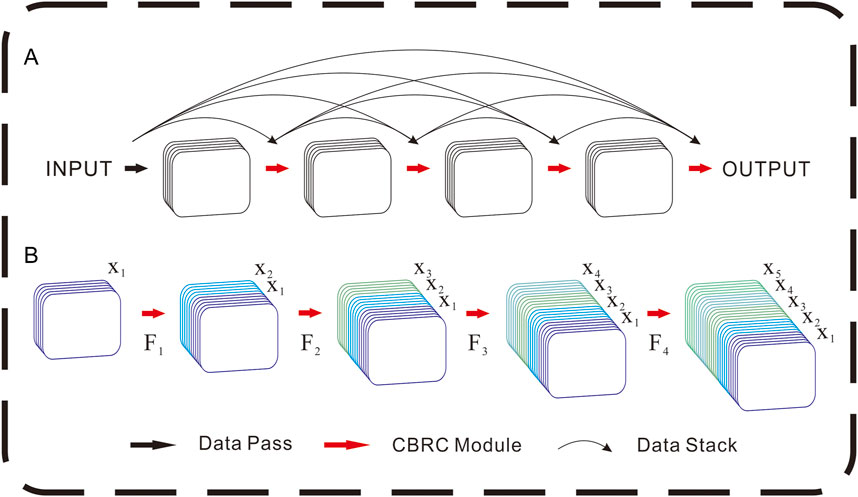
A densely connected convolutional network (Densenet) is a radical, densely connected network whose core is to establish “short-circuit connections” between the front and back layers that can reverse propagation gradients. A short circuit connection means that the front layer and the back layer directly use concatenate for channel connection so that the front layer can directly transmit the extracted features to the back layer without reservation to realize the goal of feature reuse (so as) to obtain a better calculation effect and better performance under the condition of fewer parameters and lower calculation cost.

Densenet’s connection mechanism is that all computing layers are connected in a dense block, in which computing in each layer receives all previous layers as input. Subsequently, the multiple dense blocks were connected and combined with the transition layer to form the overall Densenet network architecture.

The dense block mechanism and structure are shown in Figure 4. In picture A) of Figure 4, the black arrow represents data transmission in the figure, and the red arrow represents the Channel-BN-Relu-Conv (CBRC) module, which means batch normalization after channel stacking. The ReLU function is the activation function, and the final stride is 3×3 convolution. In picture B) of Figure 4, it is the detail of dense block shape growth and the explanation. The black trend line represents the stacking direction. The mathematical formula is described as Eq. 12:

$x_l=F_l\left(\left[x_1,x_2,x_3,\dots ,x_{l-1}\right]\right).(12)$

FIGURE 4

FIGURE 4. Dense block mechanism (A) and its details of data shape growth (B).

Among them, the $F_l$ mathematical function expression of the CBRC module $\left[x_1,x_2,x_3,\dots ,x_{l-1}\right]$ is said to $x_1,x_2,x_3,\dots ,x_{l-1}$ channel superposition.

Through such dense connection mechanisms, Densenet realized gradient backpropagation, improved the training ease of the network, made the network more robust, effectively reduced the gradient disappearance effect, and improved the robustness of the model. At the same time, when the number of sample datasets is small, the feature utilization rate is improved and the calculation is more efficient.

Therefore, this study found the excellence of Densenet, and the dense block, the core of Densenet, was extracted and nested in the D-Unet model to achieve better performance. Pleiss et al. (2017) proposed a method to reduce GPU memory consumption and graphics card requirements.

2.2.4 D-Unet model generation

Based on the aforementioned two sections, the D-Unet network architecture used in this study is finally generated. Just as in Figure 2, we use the dense blocks to replace conventional convolution layers instead. The connection between the network backbone of Unet and the dense block is for direct data transmission and no other processing. It is the core of our DL network.

D-Unet network architecture of input into two parts, respectively, is simulated high level after upward continuation of potential field data and Tikhonov regularization downward continuation after the initial model of joint as D-Unet input, output, and low wave-number domain forward generate theory plane do supervision and learning potential field data, improve the learning ability and generalization ability of the models and robustness.

After two parts of data were input into the D-Unet network, rapid feature extraction was carried out through a dense block. Convolution and maximum pooling were carried out after an enormous number of features were extracted from a small number of samples. The aforementioned steps were repeated three times to form the coding part in the sense of the traditional Unet network. When the network reaches the deepest point, the convolution operation is carried out again, and the drop out method is used to prevent the neural network from overfitting. Then the decoding part of the Unet network is used for upsampling to recover data dimensions. In the decoding part of the operation process, the concat operation of the Unet network is restored, and the encoding and decoding features are related to improving the model’s generalization ability.

2.3 Dataset network training

The forward calculation of the potential field is a linear relationship, which can be used 0.5 times and two times linear amplification of 2,000 pairs of sample data constructed in Section 2.1 to generate 6,000 theoretical datasets, forming the initial training dataset. The final dataset was randomly divided into the training part, verification part, and test data part, with a ratio of 18:1:1, which means 5,400 pieces of data participated in the training, 300 pieces of data were verified, and 300 pieces of data were tested in the final model. In data processing, all the data to be used should be normalized [0,1] first and then brought into the model. After combining the models in Section 2.2, training parameters were set, in which the number of training rounds was 50, batch size was 16, and the Adam optimizer (Kingma and Ba, 2014) was used as the optimizer in the model.

This study’s training method and effect test include the number of input channels and whether it is training with noisy samples. The image processing model of the traditional Unet network and its variants is mainly single-channel RGB input and single-channel output, that is, mapping from single image to single image, and its lack of directivity may lead to reduced convergence ability. This study hypothesizes that when the high plane potential field data and the low one are jointly driven and input into the DL network, the error between the initial model and the theoretical potential field data is small, which provides high targeting, enables the model to converge faster, and improves the generalization ability of the model. Therefore, the model experiment in this study compares whether the model input is a single channel. In addition, the generalization ability and robustness of the proposed method are tested by comparing the noiseless sample data training model with the noise-containing sample data training model.

In this study, the evaluation index of the model training effect is the root mean square error (RMSE), which is the mean square error between the results of model operation and theoretical data, and this is the loss function. Formula Eq. 13 expresses the mean square error:

$RMSE=\sqrt{\frac{1}{n}{\displaystyle \sum }_{i=1}^n{\left(m_i-{\widehat{m}}_i\right)}^2},(13)$

where $n$ indicates the number of potential field parameters, $m_i$ indicates the theoretical low plane potential field value after normalization, and ${\widehat{m}}_i$ indicates the experimental low plane potential field value obtained after normalized model training.

3 Results

3.1 Results of the theoretical model experiment

3.1.1 Comparison between deep learning and traditional continuation methods

This study adopts four different types of the particular abnormal body produced by theories of gravity data, including three significant rectangular anomalies (case 1), seven medium-sized rectangular abnormal exceptions (case 2), five medium-sized rectangular abnormal exceptions (case 3), and nine small rectangular exceptions (case 4), to test the deep learning method and the continuation of traditional continuation method ability. The deep learning method is the joint-driven method (2 input) of the D-Unet model, the conventional continuation method is Tikhonov regularization, and the evaluation index is RMSE. Figure 5 shows the comparison. The RMSE results are shown in Table 1. In the figure, a represents theoretical low plane potential field data, b represents Tikhonov potential field data, and c represents joint-driven potential field data.

FIGURE 5

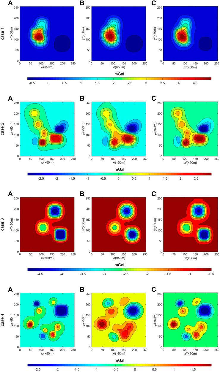
FIGURE 5. Comparison of four different cases between theoretical potential field data (A), Tikhonov regularization (B), and joint driven data (2 input) (C).

TABLE 1

TABLE 1. RMSE index comparison of the Tikhonov regularization method and joint driven input (2 input).

As shown in Figure 5 and Table 1, the continuation method trained by the deep learning D-Unet model with a joint drive significantly improves the continuation accuracy of the potential field. When the input is the joint drive, the average accuracy increases by 24.3%. Therefore, it can be inferred that the D-Unet method has a relatively noticeable improvement in the continuation of the potential field.

3.1.2 Joint drive model checking

The joint-drive model test was divided into the single input control group (1 input) and the combined drive input (2 input) experimental group. The basic model has the same parameters except for the dimensions of input parameters, and the final mapping output data have the exact dimensions. After datasets were allocated according to the allocation method mentioned in 2.1.4, they were brought into the model for training.

In the 2 input mode, the average single-round time of the 50-round model training is 116 $s$, and the continuation time of a single dataset is 21.5 $us$. The continuation speed and theoretical mathematical method are significantly improved. The trend of loss value of the training set (Loss) and loss value of the verification set (Val_Loss) with a mean square error indicator as the loss function is shown in Figure 6.

FIGURE 6

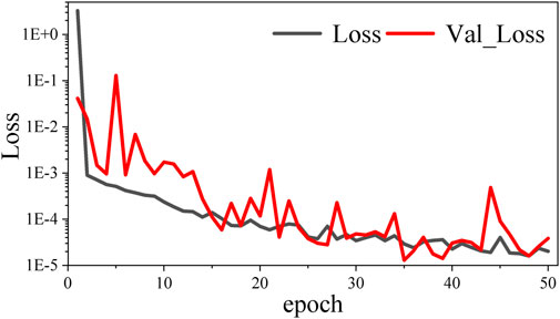
FIGURE 6. Trend of loss value of the training set (Loss) and loss value of the verification set (Val_Loss) with the mean square error indicator as the loss function in the 2 input mode.

In the 1 input mode, the average single-round time of 50-round model training is 105 s, and the continuation time of a single dataset is 21.5 us. The trend of loss value of the training set and loss value of the verification set (Val_Loss) with a mean square error indicator as the loss function is shown in Figure 7.

FIGURE 7

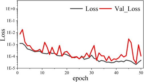
FIGURE 7. Trend of loss value of the training set (Loss) and loss value of the verification set (Val_Loss) with the mean square error indicator as the loss function in the 1 input mode.

According to the comparison of b and c in Figure 8 and the RMSE data in Table 2, the model training and continuation of single potential field continuation data have a slow speed in the convergence process due to the lack of targeting target guidance. In addition, due to the small amount of sample data, the generalization performance is not obvious enough and there is an apparent boundary anomaly, which leads to the inferior effect of the Tikhonov regularization method. Meanwhile, the results of the joint drive have the initial model to provide targeting information, which significantly accelerates the convergence speed of model training. Furthermore, it can be seen from Figure 6 that the loss curves of the model dataset and the loss curves of the verification set coincide with each other without an overfitting phenomenon. Nevertheless, the average accuracy of model continuation is improved by 24.3% through the joint drive. Therefore, it can be inferred that the joint driving method is helpful to the downward continuation of the potential field.

FIGURE 8

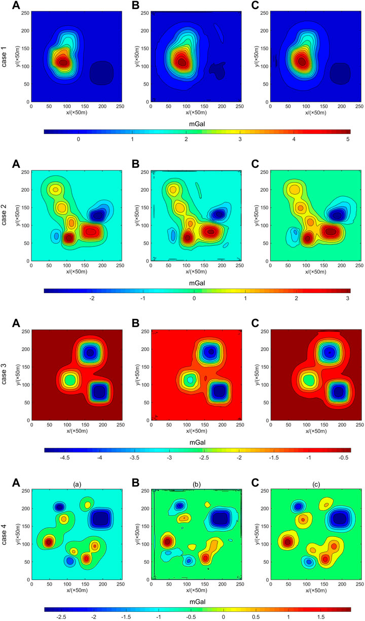
FIGURE 8. Comparison of four different cases between theoretical potential field data (A), single input (1 input) (B), and joint driven data (2 input) (C).

TABLE 2

TABLE 2. RMSE index compares single data input (1 input) and joint driven input (2 input).

3.1.3 Addition of a noise training test

Through the verification of the first two sections, it can be seen that the continuation accuracy of the joint drive method (2 input) has reached a high level. However, various disturbances in the actual working process will disturb many actual potential field values, resulting in certain noises. Therefore, 5% Gaussian noise was added to 10% random samples of the original dataset to train the model. The training parameters and process are the same as the aforementioned joint driving method, and 50 training rounds are trained. The trend of the loss value of the training set (Loss) and loss value of the verification set (Val_Loss) with a mean square error indicator as the loss function is shown in Figure 9.

FIGURE 9

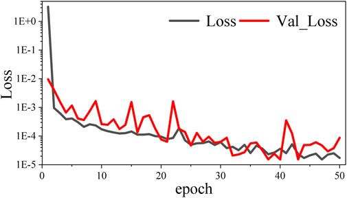
FIGURE 9. Trend of loss value of the training set (Loss) and loss value of the verification set (Val_Loss) with a mean square error indicator as the loss function in the 2 input mode with noise.

As shown in Figure 10 and Table 3, when noise samples are added to the training, the precision of model continuation is significantly improved compared with the joint drive method of the theoretical model and higher than the traditional Tikhonov regularization method. It can be seen that the addition of noise training improves the continuation accuracy and the robustness of the continuation process significantly compared with the joint drive training without noise.

FIGURE 10

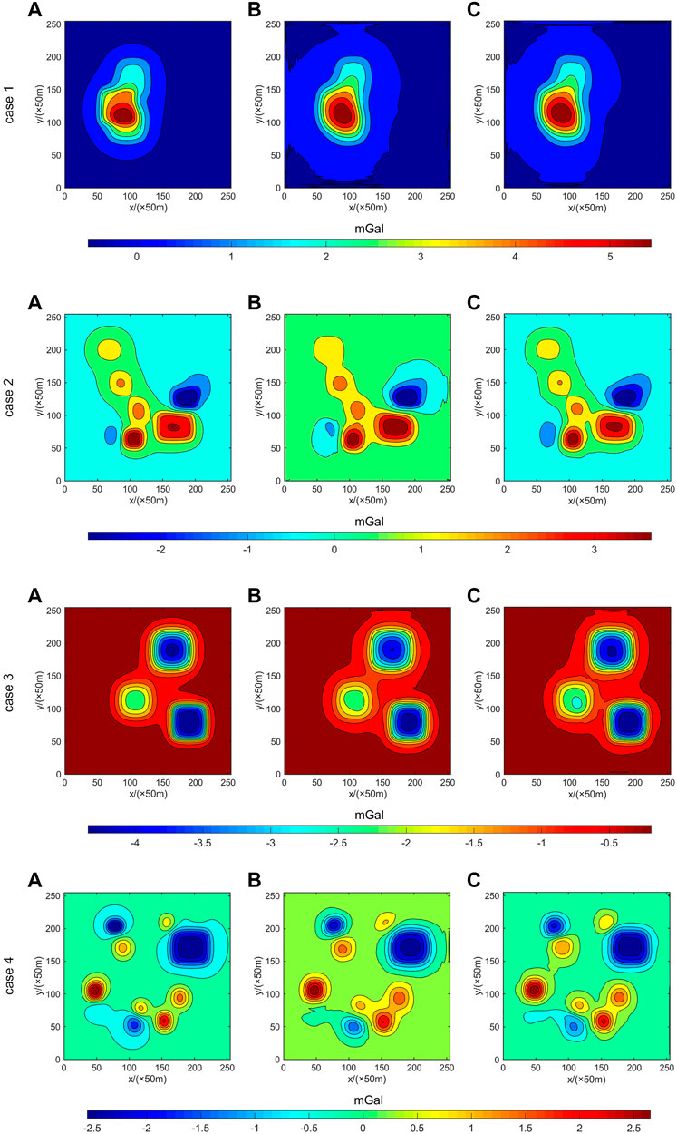
FIGURE 10. Comparison of four different cases between theoretical potential field data (A), joint driven data (2 input) (B), and joint driven data with noise (add noise) (C).

TABLE 3

TABLE 3. RMSE index compares joint driven input (2 input) and joint driven input with noise (add noise).

3.2 Results of the real example test

This study selects a particular area’s gravity potential field data in northeast China to test an example. Sun (2008) showed that this area is located in the Guomi fault zone, mainly composed of two significant faults extending roughly parallel to each other in the direction of 60° NE. They are all large angle normal faults dipping to the northwest. It is concluded that the normal northwest fault’s hanging wall (descending wall) is a negative anomaly and the footwall (uplifting wall) of the normal southeast fault is a positive anomaly. There is also a clear indication of gravity potential field data in the original low plane gravity field, as shown in Figure 11.

FIGURE 11

FIGURE 11. Actual example test data with two faults (white lines) (A) and the data continued by Tikhonov regularization (B), joint driven data (2 input) (C), and joint driven data with noise (add noise) (D).

Figure 11A shows the actual gravity potential field data selected in this study. The white lines are an indication of gravity fracture. Due to the prominent gravity anomaly on the fault zone, the error is significant. While the gravity anomaly value on both sides of the two main faults is low, there is a particular numerical leap and numerical difference. Therefore, it can be reasonably inferred that this area conforms to the description of the Guomi fault zone.

This study’s measured data take the ground gravity potential field data as theoretical data and extend it upward to simulate the aerial gravity survey’s high plane potential field data. Subsequently, the proposed D-Unet model and the joint drive method were developed and compared with the traditional Tikhonov regularization method to verify the high precision and accuracy of the proposed method.

The continuation results are shown in Figure 11, and the comparison of RMSE indexes is shown in Table 4. The figure and table show that the noised data training in the theoretical model experiment plays a role in this, and the robustness of data processing by the noised model has been dramatically improved, which exceeds the accuracy of the Tikhonov method for the continuation of the potential field. However, due to the significant noise of actual data, the joint drive model has a weak effect on noise suppression, and its continuation accuracy is slightly improved compared with the Tikhonov regularization method. It can be seen that the training of the noise-adding model is of great help to the continuation of the actual potential field.

TABLE 4

TABLE 4. RMSE index comparison after the continuation of measured data in three different methods.

4 Conclusion and prospect

1) Through the D-Unet deep learning network architecture constructed in this study and the joint driving method of high plane potential field data and Tikhonov regularization continuation data, the continuation precision of the traditional Tikhonov regularization method is improved to a certain extent, which has specific feasibility. The time consumption of the trained model is equivalent to that of the frequency domain method and it has an advantage of considerable speed over the wave-number domain method.

2) After adding noise to the training set of the joint drive model, the robustness of the model can be improved effectively, the convergence ability of the model for potential field continuation is more vital, and the suppression effect on noise is more pronounced.

3) The D-Unet deep learning method and the joint drive method were brought into the actual data of a particular area in the Guomi fault zone of northeast China for practical operation tests. The results show that the adaptability of this method to the actual situation is greatly improved compared with the traditional Tikhonov regularization method and it is feasible in the field.

4) As the reason for the case in this study that the single input effect in the model test in this study is not as good as the Tikhonov regularization method, it is suspected that the convergence may be too slow. The model may be overfitting due to the small amount of sample data and lack of targeted targets. Given this situation, we will continue the research on dataset construction and model construction and modification in the follow-up research.

5) The excellent ability reflected by the joint drive method in this study demonstrates that the joint drive method can be actively applied to other fields to achieve better results in the future combination of deep learning and different directions of geophysics.

Data availability statement

The raw data supporting the conclusions of this article will be made available by the authors, without undue reservation.

Author contributions

ZY and ZZ contributed to conception and design of the study. ZY designed and built the DL models and organized the database. ZY wrote the original draft of the manuscript. WL contributed to generate the pictures needed for the paper. ZY, ZZ, BW, WL, HL, ZS, and JL contributing to revision, read, and approved the manuscript.

Funding

This research is jointly supported by the Student Research Training Program of Southwest Jiaotong University (202110613059) and the Science and Technology Planning Project of the Sichuan Provincial Department of Science and Technology (2021YJ0031).

Conflict of interest

The authors declare that the research was conducted in the absence of any commercial or financial relationships that could be construed as a potential conflict of interest.

Publisher’s note

All claims expressed in this article are solely those of the authors and do not necessarily represent those of their affiliated organizations, or those of the publisher, the editors, and the reviewers. Any product that may be evaluated in this article, or claim that may be made by its manufacturer, is not guaranteed or endorsed by the publisher.

References

An, Y., and Guan, Z. (1985). The regularized stable factors of removing high frequency disturbances. Comput. Tech. Geophys. Geochem. Explor. 11.

Google Scholar

Bahdanau, D., Cho, K., and Bengio, Y. (2014). Neural machine translation by jointly learning to align and translate. arXiv Prepr. arXiv:1409.0473. doi:10.48550/arXiv.1409.0473

CrossRef Full Text | Google Scholar

Bateman, H. (1946). Some integral equations of potential theory. J. Appl. Phys. 17, 91–102. doi:10.1063/1.1707698

CrossRef Full Text | Google Scholar

Bhattacharyya, B. K., and Chan, K. C. (1977). Reduction of magnetic and gravity data on an arbitrary surface acquired in a region of high topographic relief. Geophysics 42, 1411–1430. doi:10.1190/1.1440802

CrossRef Full Text | Google Scholar

Chen, S., and Xiao, P. (2007). Wavenumber domain generalized inverse algorithm for potential field downward continuation. Chin. J. Geophys. 50, 1571–1579. (in Chinese). doi:10.1002/cjg2.1177

CrossRef Full Text | Google Scholar

Clarke, G. K. C. (1969). Optimum second-derivative and downward-continuation filters. Geophysics 34, 424–437. doi:10.1190/1.1440020

CrossRef Full Text | Google Scholar

Cooper, G. (2004). The stable downward continuation of potential field data. Explor. Geophys. 35, 260–265. doi:10.1071/EG04260

CrossRef Full Text | Google Scholar

Dahl, G. E., Yu, D., Deng, L., and Acero, A. (2011). Context-dependent pre-trained deep neural networks for large-vocabulary speech recognition. IEEE Trans. Audio Speech Lang. Process. 20, 30–42. doi:10.1109/TASL.2011.2134090

CrossRef Full Text | Google Scholar

Dampney, C. (1969). The equivalent source technique. Geophysics 34, 39–53. doi:10.1190/1.1439996

CrossRef Full Text | Google Scholar

Emilia, D. A. (1973). Equivalent sources used as an analytic base for processing total magnetic field profiles. Geophysics 38, 339–348. doi:10.1190/1.1440344

CrossRef Full Text | Google Scholar

Guo, L., Meng, X., Shi, L., and Chen, Z. (2012). Preferential filtering method and its application to Bouguer gravity anomaly of Chinese continent. Chin. J. Geophys. (in Chinese) 55, 4078–4088. doi:10.6038/j.issn.0001-5733.2012.12.020

CrossRef Full Text | Google Scholar

Han, W., Zhou, Y., and Chi, Y. (2018). Deep learning convolutional neural networks for random noise attenuation in seismic data. Geophysical Prospecting for Petroleum 57, 862–869. doi:10.3969/j.issn.1000-1441.2018.06.008

CrossRef Full Text | Google Scholar

Hinton, G., Deng, L., Yu, D., Dahl, G. E., Kingsbury, B., Jaitly, N., et al. (2012a). Deep neural networks for acoustic modeling in speech recognition: The shared views of four research groups. IEEE Signal Process. Mag. 29, 82–97. doi:10.1109/MSP.2012.2205597

CrossRef Full Text | Google Scholar

Hinton, G. E., and Salakhutdinov, R. R. (2006). Reducing the dimensionality of data with neural networks. Science 313, 504–507. doi:10.1126/science.1127647

PubMed Abstract | CrossRef Full Text | Google Scholar

Hinton, G. E., Srivastava, N., Krizhevsky, A., Sutskever, I., and Salakhutdinov, R. R. (2012b). Improving neural networks by preventing co-adaptation of feature detectors. arXiv preprint arXiv1207.0580. doi:10.48550/arXiv.1207.0580

CrossRef Full Text | Google Scholar

Hou, C., Cai, Z., and Liu, K. (1985). Establishing aninterpretation system of potential field transformation on anuneven surface from the potential of a single layer. Computing Techniques for Geophysical and Geochemical Exploration 1985, 99–107.

Google Scholar

Hou, C., Cai, Z., and Liu, K. (1984). Potential transformation techniques on an undulating observed profile. Chinese Journal of Geophysics 1984, 573–581.

Google Scholar

Huang, G., Liu, Z., Van Der Maaten, L., and Weinberger, K. Q. (2017). Densely connected convolutional networks. Proceedings of the IEEE conference on computer vision and pattern recognition 2017, 4700–4708.

CrossRef Full Text | Google Scholar

Hunag, Y., Wang, W., and Yu, C. (2009). Processing and transform of 3-D arbitrarily distributed potential filed data using an equivalent source approach. Progress in Geophysics 24, 7. doi:10.1016/S1874-8651(10)60080-4

CrossRef Full Text | Google Scholar

Ivan, M. (1994). Upward continuation of potential fields from a polyhedral surface1. Geophys. Prospect. 42, 391–404. doi:10.1111/j.1365-2478.1994.tb00217.x

CrossRef Full Text | Google Scholar

Kingma, D. P., and Ba, J. (2014). Adam: A method for stochastic optimization. arXiv preprint arXiv1412.6980. doi:10.48550/arXiv.1412.6980

CrossRef Full Text | Google Scholar

Krizhevsky, A., Sutskever, I., and Hinton, G. (2012). ImageNet classification with deep convolutional neural networks. Advances in neural information processing systems 25.

Google Scholar

Lecun, Y., Bengio, Y., and Hinton, G. (2015). Deep learning. Nature 521, 436–444. doi:10.1038/nature14539

PubMed Abstract | CrossRef Full Text | Google Scholar

Li, M., Li, Y., Wu, N., Tian, Y., and Wang, T. (2020). Desert seismic random noise reduction framework based on improved PSO–SVM. Acta Geod. Geophys. 55, 101–117. doi:10.1007/s40328-019-00283-3

CrossRef Full Text | Google Scholar

Li, S., Liu, B., Ren, Y., Chen, Y., Yang, S., Wang, Y., et al. (2019). Deep-learning inversion of seismic data. arXiv preprint arXiv1901.07733. doi:10.48550/arXiv.1901.07733

CrossRef Full Text | Google Scholar

Li, X., Chen, H., Qi, X., Dou, Q., Fu, C. W., and Heng, P. A. (2018). H-DenseUNet: Hybrid densely connected UNet for liver and tumor segmentation from CT volumes. IEEE Trans. Med. Imaging 37, 2663–2674. doi:10.1109/TMI.2018.2845918

PubMed Abstract | CrossRef Full Text | Google Scholar

Liang, J. (1989). Downward continuation of regularization methods for potential fields. Chinese Journal of Geophysics (in Chinese) 1989, 600–608.

Google Scholar

Liu, B., Jiao, X., and Wang, C. (1990). Boundary element method for downward continuation of potential field. Oil Geophysical Prospecting 6.

Google Scholar

Liu, J. (2008). Development new technologies for potential field processing and research on the tectonic recognition & division of ShanXi fault basin. Dissertation (Xi'an, China: Chang'an university).

Liu, T., Yang, Y., Li, Y., Feng, J., and Wu, X. (2007). The order-depression solution for large-scale integral equation and its application in the reduction of gravity data to a horizontal plane. Chinese J. Geophys. 50, 275–281. doi:10.1002/cjg2.1033

CrossRef Full Text | Google Scholar

Long, J., Shelhamer, E., and Darrell, T. (2015). Fully convolutional networks for semantic segmentation. IEEE Trans. Pattern Anal. Mach. Intell. 39, 640–651. doi:10.1109/tpami.2016.2572683

CrossRef Full Text | Google Scholar

Lou, H. (2001). The Application of gravity methods in the Investigation of crustal structure. Dissertation (Beijing, China: Institute of Geophysics, China Earthquake Administration).

Luan, W. (1983). The stabilized algorithm of the analytic continuation for the potential field. Chinese Journal of Geophysics (in Chinese) 1983, 263–274.

Google Scholar

Ma, T., Chen, L., Wu, M., and Hu, X. (2013). The selection of regularization parameter in downward continuation of potential field based on L-curve method. Progress in Geophysics 28, 2485–2494. doi:10.6038/pg20130527

CrossRef Full Text | Google Scholar

Mao, X., and Wu, R. (1998). Oscillation mechanism of potential field downward continuation in frequency domain and its elimination. Oil Geophysical Prospecting 33, 230–237.

Google Scholar

Pawlowski, R. S. (1995). Preferential continuation for potential-field anomaly enhancement. Geophysics 60, 390–398. doi:10.1190/1.1443775

CrossRef Full Text | Google Scholar

Peters, L. J. (1949). The direct approach to magnetic interpretation and its practical application. Geophysics 14, 290–320. doi:10.1190/1.1437537

CrossRef Full Text | Google Scholar

Pleiss, G., Chen, D., Huang, G., Li, T., Van Der Maaten, L., and Weinberger, K. Q. (2017). Memory-efficient implementation of densenets. arXiv preprint arXiv1707.06990.

Google Scholar

Puzyrev, V. (2019). Deep learning electromagnetic inversion with convolutional neural networks. Geophys. J. Int. 218, 817–832. doi:10.1093/gji/ggz204

CrossRef Full Text | Google Scholar

Qiu, Y., Nie, L., and Zhang, B. (2017). A practical algorithm for upward continuation of local gravity anomalies. Science of Surveying and Mapping 42, 39–42+60. doi:10.16251/j.cnki.1009-2307.2017.04.007

CrossRef Full Text | Google Scholar

Ronneberger, O., Fischer, P., and Brox, T. (2015). “U-net: Convolutional networks for biomedical image segmentation,” in International Conference on Medical image computing and computer-assisted intervention (Berlin, Germany: Springer), 234–241.

CrossRef Full Text | Google Scholar

Sun, P. (2008). Generalized gravity gradient's application and amelioration. Master’s thesis. Changchun, China: Jilin University.

Google Scholar

Sun, Y., Wang, X., and Tang, X. (2014). “Deep learning face representation from predicting 10,000 classes,” in Proceedings of the IEEE conference on computer vision and pattern recognition, 1891–1898.

CrossRef Full Text | Google Scholar

Sutskever, I., Vinyals, O., and Le, Q. V. (2014). Sequence to sequence learning with neural networks. Advances in neural information processing systems 27.

Google Scholar

Syberg, F. (1972). Potential field continuation between general surfaces. Geophys. Prospect. 20, 267–282. doi:10.1111/j.1365-2478.1972.tb00632.x

CrossRef Full Text | Google Scholar

Tian, C., Fei, L., Zheng, W., Xu, Y., Zuo, W., and Lin, C.-W. (2020). Deep learning on image denoising: An overview. NEURAL NETWORKS 131, 251–275. doi:10.1016/j.neunet.2020.07.025

PubMed Abstract | CrossRef Full Text | Google Scholar

Tikhonov, A. N., Arsenin, V. J., Arsenin, V. I. A. k., and Arsenin, V. Y. (1977). Solutions of ill-posed problems. New York, NY, USA: Vh Winston.

Google Scholar

Tong, Z., Li, Y., Li, Y., Fan, K., Si, Y., and He, L. (2020). “New network based on Unet++ and Densenet for building extraction from high resolution satellite imagery,” in IGARSS 2020-2020 IEEE International Geoscience and Remote Sensing Symposium (Waikoloa, HI, USA: IEEE), 2268–2271.

Google Scholar

Vaníček, P., Novák, P., Sheng, M., Kingdon, R., Janák, J., Foroughi, I., et al. (2017). Does Poisson’s downward continuation give physically meaningful results? Stud. Geophys. Geod. 61, 412–428. doi:10.1007/s11200-016-1167-z

CrossRef Full Text | Google Scholar

Wang, H., Yan, J., Fu, G., and Wang, X. (2020). Current status and application prospect of deep learning in geophysics. Progress in Geophysics(in Chinese) 35, 642–655. doi:10.6038/pg2020CC0476

CrossRef Full Text | Google Scholar

Wang, X., and Tian, Y. (2010). Autonomous navigation based Geomagnetic research. CHINESE JOURNAL OF GEOPHYSICS 53, 2724–2731. doi:10.3969/j.issn.0001-5733.2010.11.020

CrossRef Full Text | Google Scholar

Wang, Y. (2007). Computational methods for inversion problems and their applications. Beijing, China: Higher Education Press.

Google Scholar

Wang, Y., Wang, Z., Zhang, F., Meng, L., Zhang, J., and Tai, Z. (2012). Derivative-Iteration method for downward continuation of potential fields. Journal of Jilin University(Earth Science Edition) 42, 240–245. doi:10.13278/j.cnki.jjuese.2012.01.020

CrossRef Full Text | Google Scholar

Xi, X., and Huang, J. (2018). Deep learning inversion imaging method for scattered wavefield. Progress in Geophysics 33, 2483–2489. doi:10.6038/pg2018BB0531

CrossRef Full Text | Google Scholar

Xia, J., Sprowl, D. R., and Adkins-Heljeson, D. (1993). Correction of topographic distortions in potential-field data: A fast and accurate approach. Geophysics 58, 515–523. doi:10.1190/1.1443434

CrossRef Full Text | Google Scholar

Xiong, W. (2016). Magnetic potential field conversion method research and application. Master’s thesis (Chengdu, China: Chengdu University of Technology).

Xu, S. (2007). A comparison of effects between the iteration method and FFT for downward continuation of potential fields. Chinese J. Geophys. 50, 270–274. doi:10.1002/cjg2.1032

CrossRef Full Text | Google Scholar

Xu, S., Shen, X., Zou, L., and Yang, H. (2004). Downward continuation of aeromagnetic anomaly from flying altitude to terrain. Chinese J. Geophys. 47, 1272–1276. doi:10.1002/cjg2.614

CrossRef Full Text | Google Scholar

Xu, S. (2006). The integral-iteration method for continuation ofpotential field. Chinese Journal of Geophysics 2006, 1176–1182. doi:10.3321/j.issn:0001-5733.2006.04.033

CrossRef Full Text | Google Scholar

Yang, W. (1997). Theory and methods of geophysical inversion. Bath, UK: Geological Publishing House.

Google Scholar

Yin, B., Wang, W., and Wang, L. (2015). Review of deep learning. Journal of Beijing University of Technology 41, 48–59. doi:10.11936/bjutxb2014100026

CrossRef Full Text | Google Scholar

Yu, H. (2009). The rapid inversion of 3D apparent physical properties for potential field anomalies. Dissertation (Zhejiang, China: Zhejiang University).

Zeng, X., Fang, Y., Wang, H., and Chen, C. (2009). Slide mode guidance of infrared missile based on IMM_UKF. Journal of Astronautics 30, 7. doi:10.3873/j.issn.1000-1328.2009.04.002

CrossRef Full Text | Google Scholar

Zeng, X., Li, X., Han, S., and Liu, D. (2011a). A comparison of three iteration methods for downward continuation of potential fields. Progress in Geophysics 26, 908–915. doi:10.3969/j.issn.1004-2903.2011.03.016

CrossRef Full Text | Google Scholar

Zeng, X., Li, X., Liu, D., and Han, S. (2011b). Regularization analysis of integral iteration method and the choice of its optimal step-length. Chinese Journal of Geophysics 54, 2943–2950. doi:10.3969/j.issn.0001-5733.2011.11.024

CrossRef Full Text | Google Scholar

Zeng, X., Li, X., Niu, C., and Liu, D. (2013). Regularization-integral iteration in wavenumber domain for downward continuation of potential fields. Oil Geophysical Prospecting 48, 643–650. doi:10.13810/j.cnki.issn.1000-7210.2013.04.020

CrossRef Full Text | Google Scholar

Zeng, X., Liu, D., Li, X., Niu, C., Yang, X., and Lu, S. (2014). An improved iterative Wiener filter for downward continuation of potential fields. Chinese Journal of Geophysics 57, 1958–1967. doi:10.6038/cjg20140626

CrossRef Full Text | Google Scholar

Zhang, H., Chen, L., Ren, Z., Wu, M., Lou, S., and Xu, S. (2009). Analysis on convergence of iteration method for potential fields downward continuation and research on robust downward continuation method. Chinese J. Geophys. 52, 511–518. doi:10.1002/cjg2.1371

CrossRef Full Text | Google Scholar

Zhang, Z., Liao, X., Cao, Y., Hou, Z., Fan, X., Xu, Z., et al. (2021). Joint gravity and gravity gradient inversion based on deep learning. Chinese Journal of Geophysics (in Chinese) 64, 1435–1452. doi:10.6038/cjg2021O0151

CrossRef Full Text | Google Scholar

Zhang, Z. (2013). Numerical computation method of downward continuation of potential fields. Dissertation (Zhejiang, China: Zhejiang University).

Zhang, Z., Wu, L., Wang, R., and Zhang, J. (2013a). CGNR method for potential field downward continuation. Journal of Central South University (Science and Technology) 44, 3273–3281.

Google Scholar

Zhang, Z., Xu, S., Yu, H., and Wu, L. (2013b). Study of extending methods of iteration of downward continuation in potential field. Journal of Zhejiang University(Engineering Science) 47, 918–924. doi:10.3785/j.issn.1008-973X.2013.05.027

CrossRef Full Text | Google Scholar