
95% of researchers rate our articles as excellent or good
Learn more about the work of our research integrity team to safeguard the quality of each article we publish.
Find out more
METHODS article
Front. Earth Sci. , 09 May 2022
Sec. Quaternary Science, Geomorphology and Paleoenvironment
Volume 10 - 2022 | https://doi.org/10.3389/feart.2022.889115
 Bernd R. Schöne1*
 Soraya Marali1
 Regina Mertz-Kraus1
 Paul G. Butler2
 Alan D. Wanamaker Jr3
 Lukas Fröhlich1
Shells of bivalve mollusks serve as archives for past climates and ecosystems, and human-environmental interactions as well as life history traits and physiology of the animals. Amongst other proxies, data can be recorded in the shells in the form of element chemical properties. As demonstrated here with measured chemical data (10 elements) from 12 Arctica islandica specimens complemented by numerical simulations, mistakes during sclerochronological data processing can introduce significant bias, adding a further source of error to paleoenvironmental or biological reconstructions. Specifically, signal extraction from noisy LA-ICP-MS (Laser Ablation—Inductively Coupled Plasma—Mass Spectrometry) data generated in line scan mode with circular LA spots requires a weighted rather than an arithmetic moving average. Otherwise, results can be in error by more than 41%. Furthermore, if variations of seasonal shell growth rate remain unconsidered, arithmetic annual averages of intra-annual data will be biased toward the fast-growing season of the year. Actual chemical data differed by between 3.7 and 33.7% from weighted averages. Numerical simulations not only corroborated these findings, but indicated that arithmetic annual means can overestimate or underestimate the actual environmental variable by nearly 40% relative to its seasonal range. The magnitude and direction of the error depends on the timing and rate of both seasonal shell growth and environmental change. With appropriate spatial sampling resolution, weighting can reduce this bias to almost zero. On average, the error reduction attains 80% at a sample depth of 10, 92% when 20 samples were analyzed and nearly 100% when 100 samples were taken from an annual increment. Under some exceptional, though unrealistic circumstances, arithmetic means can be superior to weighted means. To identify the presence of such cases, a numerical simulation is advised based on the shape, amplitude and phase relationships of both curves, i.e., seasonal shell growth and the environmental quantity. To assess the error of the offset induced by arithmetic averaging, Monte Carlo simulations should be employed and seasonal shell growth curves randomly generated based on observed variations.
Bivalve shells contain a wealth of information on past climates (Ivany et al., 2011; Wanamaker et al., 2012; Wang et al., 2013; Reynolds et al., 2016, 2017; Walliser et al., 2017, 2020), human-environmental interactions (Andrus, 2011; Cannon & Burchell, 2017) and ecosystems (Gillikin et al., 2017; Estrella-Martínez et al., 2019; Graniero et al., 2021) as well as individual life histories (Jones & Gould, 1999; Moss et al., 2021; Palmer et al., 2021) and physiology of bivalves (Purroy et al., 2018). Respective data are encoded in the shells as variable increment width (Witbaard et al., 1997), microstructure (Höche et al., 2021) and chemical properties (Weidman et al., 1994) which can be placed into absolute temporal context by means of growth pattern analysis (Jones, 1980). While some fast-growing, short-lived species provide excellent opportunities to understand the paleoenvironmental variability on seasonal time-scales (Jolivet et al., 2015), the slow-growing, long-lived taxa are ideal to assess changes on inter-annual and decadal time-scales (Black et al., 2009). The outstanding longevity of some species such as Arctica islandica (up to 500 years; Wanamaker et al., 2008; Butler et al., 2013) has received particular attention, because their shells can provide insights into cycles and trends over long, uninterrupted intervals of time (Schöne, 2013). Specifically, this is the case if individual annual increment width series are combined by means of crossdating to form replicated chronologies covering many centuries or even millennia (Witbaard et al., 1997; Marchitto et al., 2000; Black et al., 2016, 2019). In recognition of this immense potential for various different disciplines, bivalve sclerochronology elicited broad resonance and gained a remarkable momentum (recent review in Peharda et al., 2021).
Parallel to progress in the field of sclerochronology, advances in analytical techniques enabled an increasingly higher sampling resolution. For example, minimum amounts of shell powder required for light stable isotope analysis via CF-IRMS (Continuous Flow—Isotope Ratio Mass Spectrometry) range between <1 and ca. 20 µg depending on periphery, setup and calibration (Ishimura et al., 2004; Fiebig et al., 2005; Vonhof et al., 2020) which translates to µm-scale spatial sampling steps. In-situ element chemical analysis by LA-ICP-MS (Laser Ablation—Inductively Coupled Plasma—Mass Spectrometry) is often completed within areas of several tens of micrometers (Raith et al., 1996; Warter & Müller, 2017). While increasingly smaller samples can be measured, it often remains unconsidered that each of them represents different amounts of time, because shell growth rates vary during the day, year and lifetime (Goodwin et al., 2001, 2003, 2021). Therefore, annual averages may be biased toward the fast-growing portion of the year if arithmetic means are computed. This bias increases with stronger seasonal contrasts of biomineralization rate and diminishes with more uniform growth rates. Although the problem has been recognized and/or properly addressed in many previous bivalve sclerochronological studies (Elliot et al., 2003; Goodwin et al., 2003, 2004, 2010; Schöne et al., 2004, 2020; Gillikin et al., 2005; Titschack et al., 2010; García-March et al., 2011; Shirai et al., 2014; Reynolds et al., 2017; Peharda et al., 2019; Ivany & Judd, 2022), no attempt has been undertaken to quantify the bias of arithmetic averaging under different simulated growth regimes and environmental boundary conditions. Another important issue arises during an earlier step of data analysis, i.e., during signal extraction from LA-ICP-MS data that were generated in line scan mode with circular LA spots. Due to the geometry of the ablated sample portion, some shell portions along the line scan are crossed more often by the laser beam than others. If this remains unnoticed and data are filtered with an arithmetic moving average rather than a weighted moving average, results can be offset. To the best of our knowledge, the bias resulting from arithmetic smoothing has never been quantified for sclerochronological samples.
In the present paper, we have mathematically assessed both issues. Firstly, we have studied how annual averages computed from arithmetically smoothed LA-ICP-MS line scan data of bivalve shells differ from the equivalent averages filtered with a weighted moving average that considers the circular LA spot geometry. Secondly, we have quantified the bias that is introduced if changes of seasonal shell growth rates remain unconsidered and arithmetic instead of weighted annual means are computed from intra-annual samples. The present study is partly based on published element chemical data (Na, Mg, Mn, Sr, and Ba) of twelve shells of modern A. islandica shells (Marali et al., 2017a, b) amended by five additional elements (B, Al, K, Zn, and Pb). Numerical models are provided to explain and support the observed patterns, and best-practice recommendations are provided. Results of this study may serve as a guideline for processing high-resolution chemical, structural or physical data obtained from bivalve shells and potentially other biogenic (e.g., corals) or abiogenic materials (e.g., speleothems, zoned minerals) that formed at variable rate.
A total of 12 specimens of modern A. islandica were obtained by dredging from NE Iceland (ICE, 9–11 m water depth, N = 4), the Faroe Islands (FO, 20 m, N = 2), the Isle of Man (IOM, 30–57 m, N = 3) and the Gulf of Maine (GOM, 83 m, N = 3) (Table 1; map provided in Marali et al., 2017b). One bivalve from the IOM died 2 years prior to collection, all others were captured alive and shucked afterward. Shells were later processed in the laboratory. For a detailed description of the sample preparation and growth pattern analysis Marali et al. (2017a). Briefly, two approx. 3 mm-thick sections were cut from each shell, ground and polished with suspensions of F800/1200 grit SiC and 1 µm Al2O3 powder, respectively. In case of samples from NE Iceland and the Faroe Islands, one section was immersed in Mutvei’s solution and used for annual increment width measurements in the hinge (data published in Marali et al., 2017b) using a combination of sectoral dark field and fluorescent light microscopic analysis. Growth pattern analysis of the specimens from the other two localities (Butler et al., 2010; Griffin, 2012) was performed on acetate peel replicas (for analytical details Butler et al., 2009). Annual increment chronologies were used to add a calendar axis to the chemical data of the shells and determine the ontogenetic age of the studied specimens.
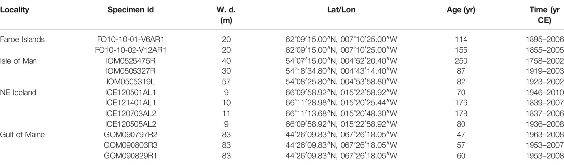
TABLE 1. Overview of shells of Arctica islandica used in present study. Except for specimen IOM0525475R, all bivalves were collected alive. W. d. = Water depth; Age = Ontogenetic age); Time = Studied time interval.
The remaining polished shell slab (hinge portion) of each specimen was used for in-situ chemical analysis by means of Laser Ablation—Inductively Coupled Plasma—Mass Spectrometry. The LA-ICP-MS system at the University of Mainz consisted of a 193 nm ArF Excimer laser (ESI NWR193) coupled to an Agilent 7500ce quadrupole ICP-MS. Measurements were performed in line scan mode at a scan speed of 5 μm/s and a beam diameter of 55 µm. The distance between laser spot positions at which a new data acquisition cycle started was approx. 1.45 µm. The laser repetition rate equaled 10 Hz and the laser energy on samples was about 7 J/cm2. During measurement, the laser penetrated approx. 15 µm deep into the sample surface. To remove potential surface contaminants, prior to measurements, sample surfaces were pre-ablated applying a spot size of 100 µm in line scan mode with 3 Hz, 50 μm/s scan speed at an energy density of about 3 J/cm2. This resulted in removal of approx. 0.6 µm of the sample surface. Background intensities were measured for 20 s prior to each line scan.
Accuracy and precision of the analyses were monitored with NIST SRM 610, USGS BCR-2G and USGS MACS-3 (for respective quality control data Supplementary Data). NIST SRM 612 was used to calibrate the element concentrations of shells and other reference materials using preferred values reported in the GeoReM database (available at http://georem.mpch-mainz.gwdg.de, ver. 30, last access: 1 March 2022; Jochum et al., 2005, 2011). Concentrations of the following elements were determined: boron (measured as intensity of 11B), sodium (23Na), magnesium (25Mg), aluminum (27Al), potassium (39K), manganese (55Mn), zinc (66Zn), strontium (88Sr), barium (137Ba), and lead (208Pb). Element-specific RSD% (relative standard deviation) values and average detection limits (computed as 3σbackground according to Jochum et al., 2012) are listed in the Supplementary Data. 43Ca served as the internal standard for reference materials and shells. Calcium concentrations for the reference materials were taken from GeoReM, for the shells data given in Marali et al. (2017a), i.e., 380,000 μg/g.
LA-ICP-MS data obtained in line scan mode show a much higher scatter (= lower signal-to-noise ratio) than results from single spot analysis along the same transect would reveal. To extract signals from such noisy data (Figure 1), digital filtering (“smoothing”, denoising) is required. Marali et al. (2017a) has accomplished this with a 31-pt moving average filter. Here, we compared results of two different smoothing approaches using a 38-pt arithmetic moving average filter and a 38-pt weighted moving average filter (Figure 1). The reason for computing the arithmetic mean of 38 (instead of the arbitrarily chosen 31 in Marali et al., 2017a) successive data points is that any given portion of the laser-scanned shell (except the first and last 27.55 µm of the line scan) was at maximum measured this many times. Because the distance between laser spot positions at which a new data acquisition cycle started equaled approx. 1.45 µm, it took 38 measurement cycles until the laser traveled 55 μm, i.e., the diameter of one LA spot (Figure 2). As a simplification and for the ease of explanation, it is assumed here that the laser beam moved stepwise rather than with continuous speed, and chemical analyses were taken at equidistant intervals of 1.45 µm, i.e., analyses were completed within individual spots where midpoints of LA spot were 1.45 µm apart from each other. Figuratively speaking, a 1.45 µm wide and 55 µm heigh (rectangular) stripe of shell located at the front edge of the first LA spot was crossed by 38 LA spots. However, due to the geometry of the laser spot on the sample surface, i.e., circles (= LA spots) with 55 µm diameter, the rectangular shell stripes (1.45 × 55 µm) were crossed by variably sized LA spot segments. Or differently expressed, some portions of the rectangular stipe of shell were measured more frequently (those near the center of the line scan) than others (near the periphery) (Figure 2). To smooth such data correctly, a circle segment area-based weighted moving average needs to be employed, not just an arithmetic moving average that assumes that the LA “spot” was rectangular. The areas of these circle segments were thus used as weighting factors for the respective element concentration data (calculation details are given in the Supplementary Data; weights listed in Figure 2). Data from laser spots near the center of a given stripe of shell were overweighted relative to such near the edge. Due to end fitting problems, the first and last 19 averages (each representing 27.55 µm of the line scan) were omitted.
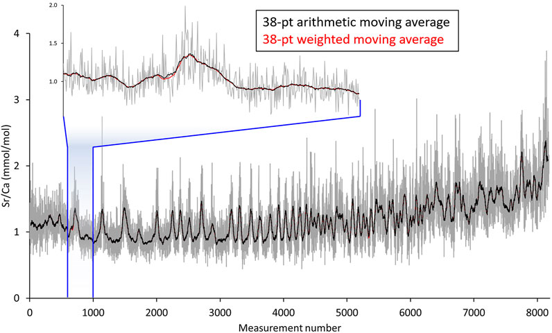
FIGURE 1. LA-ICP-MS line scan data (here molar Sr/Ca ratios, grey) of the hinge portion of Arctica islandica specimen ICE120703AL2 from NE Iceland (Table 1). Direction of growth is to the right. Signals extracted via a 38-pt arithmetic moving average slightly deviate from such obtained with a 38-pt weighted moving average that takes the circular geometry of the laser beam into account. The arithmetic average (black) preserves more noise than the weighted average (red).
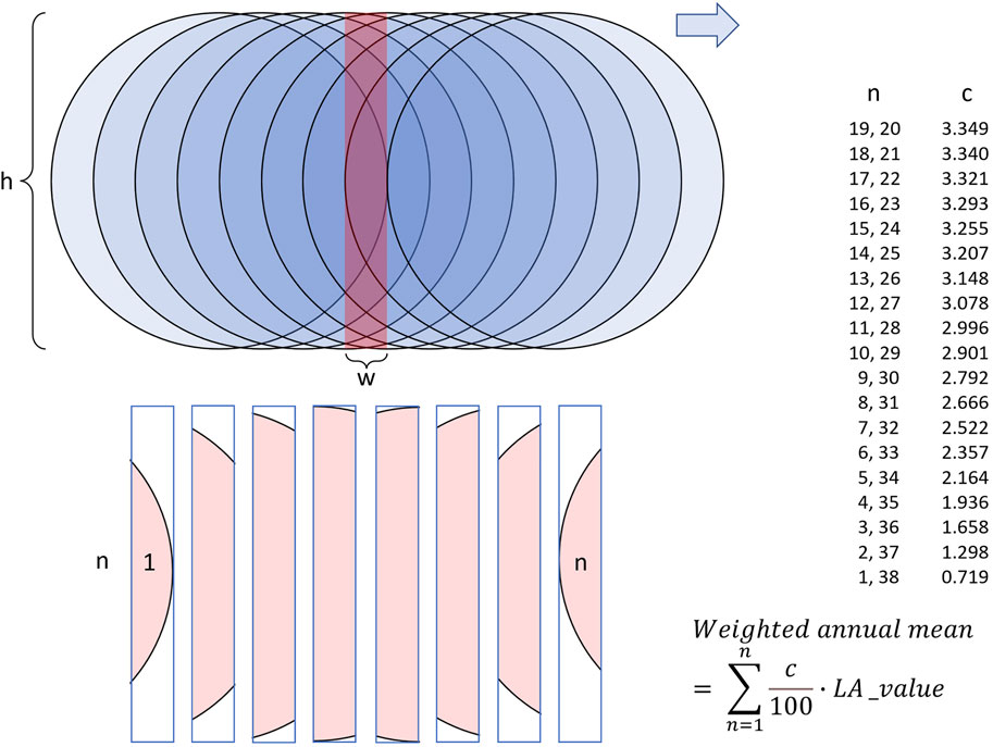
FIGURE 2. Schematic illustration of LA-ICP-MS line scan data discretization. Blue circles denote the laser spots on the sample surface. While the laser beam moves forward (here to the right) and ablates shell material, a new data acquisition cycle starts every 1.45 µm (in the setup used in this study). For simplification of the calculations, it is assumed that measurements are instantaneously completed, while in reality, measurements are integrated over some time interval while the laser continues to travel to the right. As the laser spot diameter (h) measures 55 µm and measurements are completed at regular spatial intervals (w) of 1.45 µm, each rectangular stripe of shell (red) measuring 1.45 × 55 µm is measured 38 times (note, illustration not to scale; for simplification, only eight acquisition cycles depicted). Signal extraction of the noisy LA-ICP-MS line scan data should thus be done with a symmetrical moving average integrating 38 data points. However due to the geometry of the laser beam, each rectangular stripe of shell is crossed 38 times (n) by variably sized LA spot portions (pink; note, for illustration purposes n = 8). Portions near the center of the rectangular stripe of shell are measured more frequently than those near the periphery. To denoise the data properly, a 38-pt circle segment area-based weighted moving average needs to be used. Filter weights (c) for the respective LA spot (n) are listed to the right including the respective function to smooth the data. LA_val = element chemical value measured at a LA spot.
The conversion of the continuous line scan data with overlapping sampling spots into a new chronology with non-overlapping data is known as discretization. Similar techniques as applied herein have previously been used to increase the spatial resolution of LA-ICP-MS data required to obtain a more precise understanding of the rate at which magma ascends (Fox et al., 2017).
Conversion of the digitally filtered element chemical data from the distance to the time axis can be done in two ways which were both assessed here. A common practice (also done in Marali et al., 2017a, b) is to distribute the data of samples taken at equidistant intervals (such as the discretized LA-ICP-MS line scan data) evenly across the year assuming that each data point represents the same amount of time and—within a given growing season—biomineralization rate occurred continuously and at an unchanged rate. For example, if 52 data points were measured within an annual growth increment (i.e., between two subsequent annual growth lines), each data point is assumed to comprise ca. one week, and the “annual” (= growing season) average is computed as the arithmetic mean of these 52 values. However, shell production rates typically vary substantially throughout the growing season so that time-averaging deviates between samples. To account for such seasonal changes in growth rate, water-depth specific seasonal growth models, recently provided for A. islandica by Höche et al. (2022), were applied to precisely temporally align the chemical data (Figure 3 depicts the model for NE Iceland). Gaps between the temporally aligned data were filled by linear interpolation so as to obtain daily element-to-Ca chronologies. From these data, annual averages were computed arithmetically. To consider changes in seasonal shell growth rate properly, weighted annual averages were calculated as well.
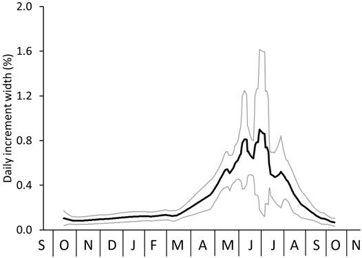
FIGURE 3. Seasonal growth model (daily resolution) of Arctica islandica from NE Iceland (average = black line; 1σ error = grey) based on 11 specimens. Data taken from Höche et al. (2022).
In summary, four different variants of annual chronologies were computed and compared to each other: 1) arithmetic annual means from arithmetically smoothed LA data, 2) arithmetic annual means from weight-smoothed LA data, 3) weighted annual means from arithmetically smoothed LA data, and 4) weighted annual means from weight-smoothed LA data. In contrast to arithmetic smoothing, weighted smoothing considers that some shell portions were measured more often than others. In contrast to arithmetic annual means, the calculation of weighted annual means considers the seasonally varying rates of shell growth.
To simulate the differences between arithmetic and weighted annual averages, numerical models were computed in which the sampling resolution (N = 1 to 100 equidistant samples), the seasonal shell growth curve as well as the data recorded in the shell were varied. To provide a tangible example, it was assumed that the bivalve perfectly (i.e., without any kinetic or vital effects) chronicled the sea surface temperature (SST) history during the growing season in its shell (in the form of “proxy-SST”). Aside from assessing differences between arithmetic and weighted proxy-SST averages, this approach also provided the possibility to contrast the shell-derived averages with the actual SST average during the growing season.
Two different model setups were assessed. In the first model, the published seasonal growth model (daily resolution) of A. islandica from NE Iceland (Figure 3; Höche et al., 2022) and instrumental SST data from that region were employed as input variables. The latter were obtained as monthly averages (1953–2021) from the NOAA Physical Sciences Laboratory from their website at www.psl.noaa.gov (data product: Extended Reconstructed Sea Surface Temperature V5; grit 66 N, 14 W) and converted to daily SST by linear interpolation. In model two, both the seasonal shell growth and environmental SST were numerically simulated with sinusoidal and gaussian functions. This provided the possibility to phase-shift the curves against each other, modulate their amplitudes, stretch or compress the curves along the time axis, and add skewness in order to assess the respective effect on arithmetic and weighted annual proxy-SST averages in comparison to the simulated environmental SST mean.
To compute a weighted annual mean from proxy-SST, the relative proportion of time represented by each intra-annual sample served as a weighting factor by which the proxy-SST value from the respective sample was multiplied. The weighted annual average could then be computed as the arithmetic mean of all weighted intra-annual proxy-SST data. Since no actual chemical measurements were used in this model, it was also necessary to simulate the growth rate-related bias contained in the (hypothetical) shell record and determine the proxy-SST value that would have been measured in a given intra-annual sample that formed at daily changing growth rates (evidently, each intra-annual proxy-SST value is likewise biased toward faster growth and differs from the arithmetic mean computed from the simulated environmental SST). This was compensated by weighting the simulated daily environmental SST data by the simulated amount of shell that formed during the respective day. To do so, each simulated daily SST value was multiplied by the corresponding simulated daily increment width. Then, weighted daily temperatures were arithmetically averaged to provide the weighted proxy-SST average of each intra-annual shell sample.
As demonstrated by the representative example depicted in Figure 4 (for full set of chronologies Supplementary Data) and the quantitative analysis of the entire dataset (Supplementary Table S1), no major role was played by the choice of which of the two discretization techniques was applied before annual means are computed from LA-ICP-MS line scan data. Annual averages calculated from data filtered with the arithmetic moving average were nearly identical to such filtered with the circle segment area-based weighted moving average. The mean difference was merely 1.0 ± 0.4% (average ± 1σ; N = 12,980), but the average of the largest differences were six times as high and equaled 5.9 ± 2.6% (N = 120, one value per element chemical chronology) (Supplementary Table S1). For elements with sharp, episodic peaks and a flat background in the raw data such as Al (Supplementary Data), the largest offset even amounted to 41.2% (on average, 14.3%; Supplementary Table S1).
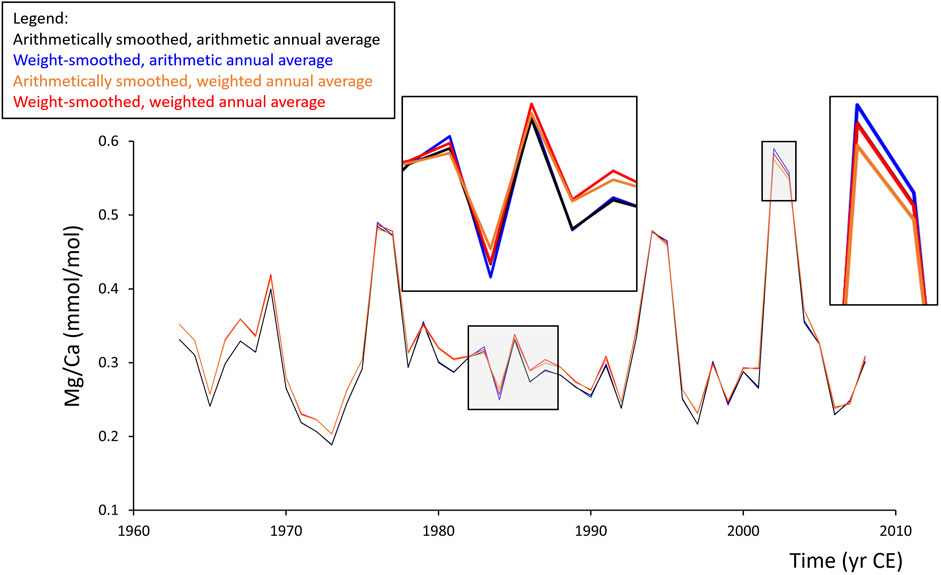
FIGURE 4. Annual Sr/Ca chronologies of A. islandica specimen GOM090797R2 from the Gulf of Maine (Table 1) computed by different data processing steps. Raw LA-ICP-MS data (acquired in line scan mode) were digitally filtered by a 38-pt arithmetic moving average as well as a 38-pt weighted moving average Figure 2). Then, arithmetic (black, blue) and weighted (orange, red) annual means were computed from both data series. While data smoothing (black vs. blue, orange vs. red) had comparatively small effects, the different methods used to compute annual means resulted in larger offsets (black/blue vs. orange/red), specifically in shell portions formed during early ontogeny.
Element chemical chronologies of shells from GOM not only were the shortest, but also showed the largest agreement among the four studied regions (average difference: 0.6 vs. 0.9–1.4%, average of the largest difference: 3.7 vs. 5.3–8.8%; Supplementary Table S1). Actually, in longer time-series, the differently filtered datasets seemed to be in stronger disagreement than in shorter chronologies, but significant (p < 0.05) positive linear correlations (R = 0.59 to 0.89; R2 = 0.35–0.80) between the offset and ontogenetic age only existed for Na, Al, K, Zn, and Pb (Supplementary Table S1; note that Al and Zn were mostly below LOD; Supplementary Data). Among the studied element-to-Ca ratios, Na/Ca series least affected by the different discretization techniques (0.2 ± 0.1% and 1.4 ± 0.6%, respectively), and Al/Ca, Mn/Ca, Zn/Ca, Ba/Ca, and Pb/Ca were most severely affected (1.1–2.4 and 7.5–14.3% difference, respectively; Supplementary Table S1). In contrast to Na, the latter elements showed larger variability with occasional strong peaks.
High-resolution proxy data measured in shells can also be combined into annual averages, for example, to identify cycles and trends through time etc. A critical aspect, however, is how these averages are computed, arithmetically or weighted. The latter technique accounts for seasonally varying growth rates and gives more weight to samples from slow-growing portions relative to such from fast-growing portions. A direct comparison of arithmetic and weighted annual means (computed from weight-filtered LA data) revealed more substantial discrepancies than those caused by the different smoothing techniques (Figure 4). Whereas the average difference was only 3.7 ± 1.8%, the average of the largest differences amounted to 33.7 ± 46.0% (Supplementary Table S2). The large standard deviation error of the latter resulted from eminent discrepancies during individual years of Al/Ca, K/Ca, Zn/Ca, and Pb/Ca in specimen IOM0505319L. However, even without these values, the average of the largest differences remained high (22.4 ± 12.1%). As before, smallest differences were observed among the GOM series (10.5 ± 2.1%), but except for Mg (negative correlation: R = −0.59, p = 0.04), the differences caused by the two temporal alignment techniques were unrelated to ontogenetic age (Supplementary Table S2). Arithmetically and weight-averaged Na/Ca chronologies were nearly indistinguishable (average difference: 0.7%; average maximum difference: 4.2%). However, other element-to-Ca data were more strongly affected by the temporal alignment technique, specifically Al, Ba, and Pb (average maximum deviations: 84.5, 51.1, and 56.9%, respectively), and to a lesser degree K, Mn, and Zn (average maximum differences: 26.8–42.3%; Supplementary Table S2).
In general, the differences caused by the smoothing techniques and annual averaging methods were larger for shell portions formed during early ontogeny, i.e., in broader increments and when sampling resolution was higher (Figure 4). Particularly, this applied to B, Mg, K, Mn, and Ba (Supplementary Table S2). These elements appeared to be more strongly positively and linearly correlated (on average, R > 0.37) with annual increment width than the remaining studied elements. However, none of the elements was statistically significantly (p < 0.05) correlated with increment width (and thus sample depth) in all twelve shells (Supplementary Table S1). In case of Ba, one shell from GOM did not reach the critical threshold, and in case of Mn, both specimens from FO and two from ICE remained below the significance level.
The differences between arithmetic and weighted annual means of samples with variable time-averaging were also assessed by numerical simulations (Figures 5–12; Supplementary Tables S1–S3). As outlined in the Materials and Methods section, in these models, the shell element chemical data is referred to as “proxy-SST” values. This terminology makes the description of the following more comprehensible and also accounts for the fact that use of element chemical properties of bivalve shells as environmental proxies is still a matter of debate (e.g., in A. islandica: Schöne, 2013; Wanamaker & Gillikin, 2019). In the first instance (Figure 5), real data were used, namely, the typical daily growth curve (= seasonal growth model) of A. islandica in NE Icelandic surface waters and the instrumental SST curve (long-term daily averages) of the same setting (Figure 5A). In shallow waters, the growing season of the ocean quahog starts in ca. mid-October. The biomineralization rate remains low until the following spring when food availability and temperature rise. Fastest shell formation rates are attained during June/July shortly after the seasonal phytoplankton bloom. Growth rate then slows down culminating in the formation of a distinct annual growth line between approx. mid-September and mid-October, i.e., the growth line formation starts about 1 month after the seasonal SST maximum (Figure 5A). Note, if growth came to a complete halt, no shell and thus, no growth lines could have formed. Though a complete interruption of biomineralization cannot entirely be precluded, we assume here that growth commenced during that time period, though at a very low rate. Due to seasonal growth rate variations, the shell record is biased toward the faster growing shell portions and spring/summer SST (Figure 5B). Temperatures during winter are therefore only encoded in a small portion of the annual increment, because the majority of the increment grew during the warm, productive part of the year (Figures 3, 5B). If this remained unconsidered, an arithmetic average computed from all samples taken at equidistant intervals from an annual increment would be notably higher than the actual annual mean (Figure 5C). Irrespective of the sampling resolution, this arithmetic average would remain unchanged. Following the numerical simulation, the offset equals almost + 1°C (5.08 vs. 6.02°C, respectively) corresponding to nearly 18% of the seasonal temperature amplitude (Figures 5C, 12; Supplementary Table S3). However, when the seasonal growth rate changes are taken into account, the weighted annual average will reflect the actual average SST much closer (Figures 5D, 12; Supplementary Table S3). With increasing sampling resolution, the error can be gradually reduced, for example, with 10 intra-annual samples to + 0.04°C or + 0.7%, and to as little as + 0.01°C or + 0.2% as soon as 20 equidistant samples are taken from the annual increment (Figures 5D, 12; Supplementary Table S3).
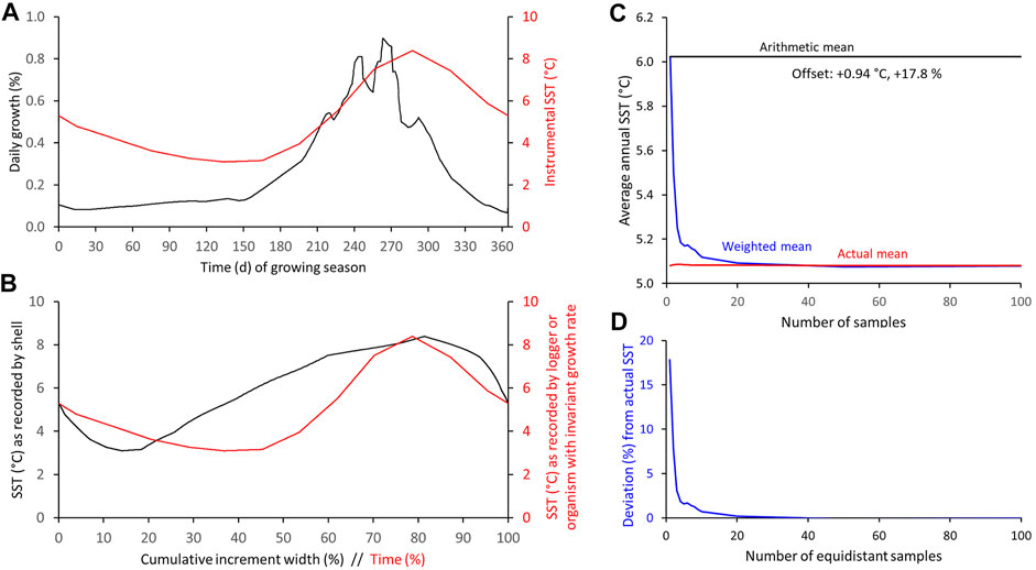
FIGURE 5. Numerical simulation of differences between arithmetic and weighted annual means computed from intra-annual proxy-SST. (A) Seasonal growth model of Arctica islandica from NE Iceland in comparison to instrumental SST. (B) SST as recorded by shell (variable seasonal growth rate) and logger. (C,D) Arithmetic and weighted annual proxy-SST in comparison to actual SST mean. With increasing sample resolution, the weighted mean agrees better with the instrumental SST average (C): absolute values; (D): relative values.
In other habitats and/or for other species, the seasonal growth and temperature curves can be much different from those presented above. For example, the phase relationship between the curves can vary, the amplitudes can vary, the curves can be compressed or stretched, skewed etc., All of these variations would affect the difference between weighted and arithmetic proxy-SST means as well as their offset from the actual SST mean measured in the environment. Such effects were simulated in an exemplary way and depicted in Figures 6–12 (also Supplementary Table S3). If shell growth (0–4 arbitrary units/day, max: 0.55%/day/annual increment width) is strongly positively coupled to water temperature (0–4°C) (Figure 6), the arithmetic SST mean (3°C) overestimates the actual SST mean (2°C) by 1 °C, i.e., by 25% relative to the seasonal SST amplitude (4°C), whereas the weighted mean merely deviates from the actual SST by one-eighth (+ 0.12°C, + 3.0%) of that value when 20 intra-annual samples are taken, and nearly matches the actual SST average (+ 0.04°C, + 0.8%) when the sample depth approaches 50 (Figure 12). If the curves are in antiphase, the signs reverse. In both cases (in-phase or in antiphase), changes of the amplitudes of seasonal shell growth rate or SST have no effect on the relative offset. However, the absolute bias of the arithmetic average changes proportionately to a change in the SST range. When the seasonal growth maximum (or minimum) occurred half-way between the seasonal SST extremes (Figure 7), the arithmetic mean would perfectly resemble the actual mean, but the weighted mean would underestimate the actual SST by up to 0.30°C (−7.7% relative to the SST amplitude) when the sample resolution was 4–5. The offset rapidly decreases as the sample depth is decreased or increased, e.g., −0.2°C (−5.8% or −5.3%) at 2 or 20, respectively, −0.1°C (−2.6%) at 50 and −0.01°C (−0.4%) at 100 equidistant samples (Figures 7, 12; Supplementary Table S3).
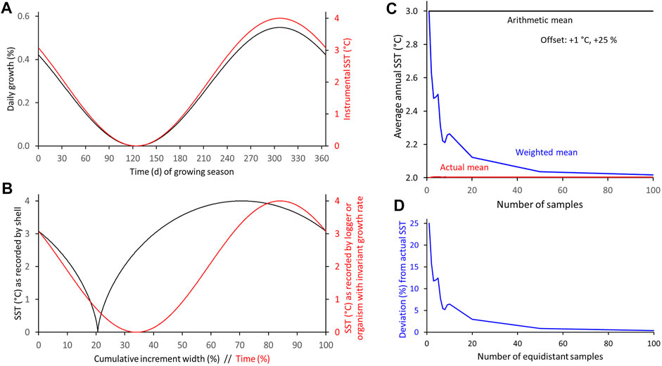
FIGURE 6. Numerical simulation of differences between arithmetic and weighted annual means computed from intra-annual proxy-SST assuming shell growth and SST curves are in phase and have a symmetrical shape. (A) Modeled seasonal shell growth and SST. (B) SST as recorded by model shell and logger. (C,D) Arithmetic and weighted annual proxy-SST in comparison to actual SST mean. With increasing sample resolution, the weighted mean agrees better with the instrumental SST average (C): absolute values; (D): relative values.
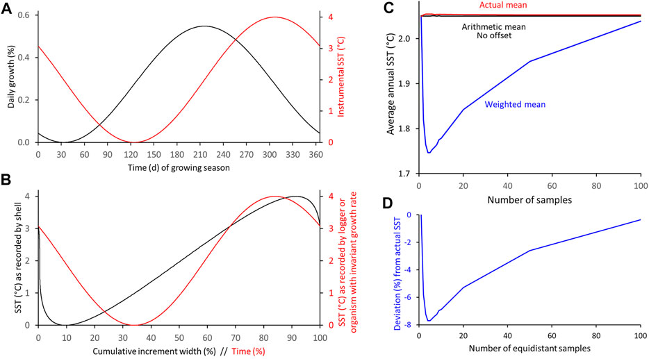
FIGURE 7. Numerical simulation of differences between arithmetic and weighted annual means computed from intra-annual proxy-SST assuming maximum shell growth occurs half-way between SST extremes and both curves are symmetrically shaped. (A) Modeled seasonal shell growth and SST. (B) SST as recorded by model shell and logger. (C,D) Arithmetic and weighted annual proxy-SST in comparison to actual SST mean. With increasing sample resolution, the weighted mean agrees better with the instrumental SST average (C): absolute values; (D): relative values.
An increasingly shorter growth period (= compressed growth curve) results in larger differences between the actual and reconstructed SST means, unless a weighted mean is computed from a sufficient number of subannual samples (Figures 8–12; Supplementary Table S3). For example, when both curves are in phase and the main growth period comprises ca. five months, the arithmetic mean overestimates the actual SST by 1.6°C (39.4% of the SST amplitude), whereas the weighted mean provides reasonable results (+ 0.1°C, + 2.6%) and near-perfect results (+ 0.01°C or + 0.2%) when a sampling resolution of 20 and 50 is applied, respectively (Figures 8, 12; Supplementary Table S3). A rapid decrease of shell formation rate after the seasonal growth maximum combined with a shortening of the main growing season to ca. three months leads to a slight decrease of the offsets (36.9% and <1.5%, respectively) (Figures 9, 12; Supplementary Table S3). When the timing of maximum shell growth is closer to that observed in A. islandica at NE Iceland and the shape of the growth curve (non-skewed) and duration of the main growing period is left unchanged (ca. five months), however, the arithmetic mean overestimates actual SST by + 1.0°C (+ 25.5%), while a weighted mean at a sample depth of 10 would return proxy-SST that merely deviate from actual SST by + 0.1°C (+ 2.3%) (Figures 10, 12; Supplementary Table S3). A left-skewed seasonal growth curve would reduce the offsets by approx. 50% (Figures 11, 12; Supplementary Table S3). If both curves are left-skewed and the maxima occur at the same time (not shown), the arithmetic mean overestimates the actual mean by nearly 1°C (25.3%) (Figure 12; Supplementary Table S3).
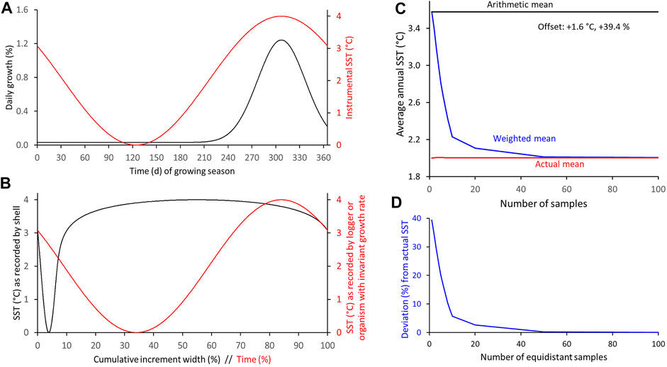
FIGURE 8. Numerical simulation of differences between arithmetic and weighted annual means computed from intra-annual proxy-SST assuming main growing season (fast growth) is limited to about 5 months, shell growth and SST curves are in phase and both have symmetrical shape. (A) Modeled seasonal shell growth and SST. (B) SST as recorded by model shell and logger. (C,D) Arithmetic and weighted annual proxy-SST in comparison to actual SST mean. With increasing sample resolution, the weighted mean agrees better with the instrumental SST average (C): absolute values; (D): relative values.
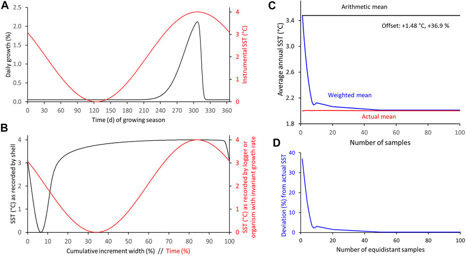
FIGURE 9. Numerical simulation of differences between arithmetic and weighted annual means computed from intra-annual proxy-SST assuming main growing season (fast growth) is limited to about 3 months, shell growth and SST curves are in phase, growth curve is left-skewed and SST curve has a symmetrical shape. (A) Modeled seasonal shell growth and SST. (B) SST as recorded by model shell and logger. (C,D) Arithmetic and weighted annual proxy-SST in comparison to actual SST mean. With increasing sample resolution, the weighted mean agrees better with the instrumental SST average (C): absolute values; (D): relative values.
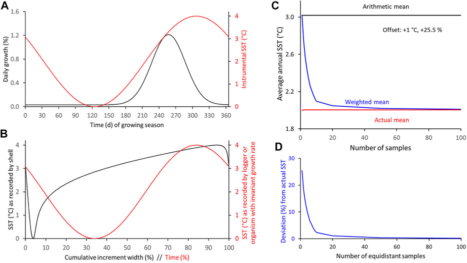
FIGURE 10. Numerical simulation of differences between arithmetic and weighted annual means computed from intra-annual proxy-SST assuming main growing season (fast growth) is limited to about 5 months, maximum shell growth occurs half-way between SST extremes and both curves are symmetrically shaped. (A) Modeled seasonal shell growth and SST. (B) SST as recorded by model shell and logger. (C,D) Arithmetic and weighted annual proxy-SST in comparison to actual SST mean. With increasing sample resolution, the weighted mean agrees better with the instrumental SST average (C): absolute values; (D): relative values.
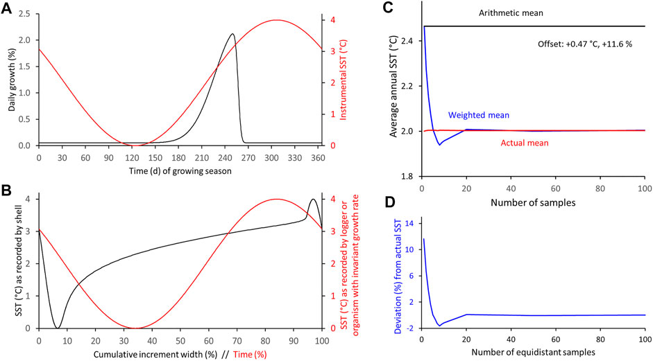
FIGURE 11. Numerical simulation of differences between arithmetic and weighted annual means computed from intra-annual proxy-SST assuming main growing season (fast growth) is limited to about 3 months, maximum shell growth occurs half-way between SST extremes, growth curve is left-skewed and SST curve has a symmetrical shape. (A) Modeled seasonal shell growth and SST. (B) SST as recorded by model shell and logger. (C,D) Arithmetic and weighted annual proxy-SST in comparison to actual SST mean. With increasing sample resolution, the weighted mean agrees better with the instrumental SST average (C): absolute values; (D): relative values.
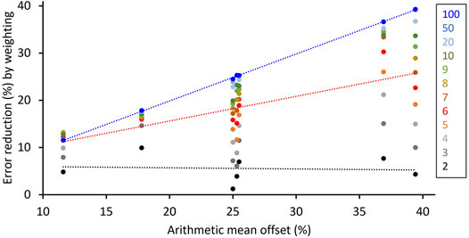
FIGURE 12. Error reduction by computing weighted instead of arithmetic means from intra-annual proxy-SST data of Arctica islandica shells as shown in Figures 5, 6, 8–11 (i.e., excluding cases where the arithmetic mean provides superior results, i.e., Figure 7). With increasing sample resolution (black to blue), the weighted mean agrees better with the instrumental SST average. Numbers in box indicate sample depth, i.e., number of intra-annual samples. For further details Supplementary Table S3.
As demonstrated here, the arithmetic averaging of bivalve shell-derived proxy data representing unequal sample sizes or different amounts of time can challenge paleoenvironmental interpretations. Specifically, signal extraction from noisy LA-ICP-MS data generated in line scan mode with circular LA spots requires a weighted rather than an arithmetic moving average (Figures 1, 4, Supplementary Table S1). In turn, if variations of shell growth rate remain unconsidered, annual averages will be biased toward the fast-growing season of the year (Figures 5–12, Supplementary Tables S2, S3). A large number of factors can potentially influence environmental proxy data recorded in bivalve shells including kinetic and vital effects, chemical inhomogeneities below the sample surface etc., Thus, any additional errors resulting from the sample spot geometry and differences in time-averaging of individual samples should be minimized. This can be accomplished with a few additional data processing steps (Figure 2) as well as a detailed analysis of the typical species and habitat-specific timing and rate of seasonal shell growth (Figure 3).
According to exemplarily studied shells of A. islandica from different localities in the North Atlantic, overall, it did not play a major role if signals were extracted from noisy LA-ICP-MS line scan data with an arithmetic or weighted moving average filter (Figure 4, Supplementary Table S1). Averaged over the ten investigated elements, the annual means computed from such datasets differed by only 1%. However, the largest offsets of the chronologies attained, on average, almost 6%, and for elements with sharp, episodic peaks in the raw data such as Al, Zn, Ba, and Zn (e.g., Stecher et al., 1996; Gillikin et al., 2008; Marali et al., 2017b), this figure was occasionally exceeded multiple times. Hence, if the data were processed with an arithmetic moving average, ephemeral signals in faster growing shell portions would get attenuated due to a flawed smoothing technique.
With increasing chronology length, the discrepancies between annual averages computed from arithmetically and circle segment area-based weight-filtered raw element-to-Ca data tended to become larger (Supplementary Table S1). Chronologies of elements with a more pronounced seasonal variance or episodic sharp peaks in the raw data were—again—particularly affected. This observation can be explained by a more pronounced change of element concentration between sample points in slower growing shell portions. An arithmetic average smooths such data less well than a weighted average as shown by an artificial data set (Supplementary Data) and in Figure 4; albeit in weakened form, the same can be observed in faster growing shell portions (Figure 1). Consequently, the offset between chronologies computed from differently smoothed raw data increases with decreasing sampling resolution (Supplementary Table S1). For this reason, the offset also increases with chronology length, because a larger proportion of narrow increments then contributes to the average error.
Based on the findings from measured data (Figure 1, Supplementary Table S1) and, more importantly, theoretical considerations (Figure 2), it is recommended here to smooth LA-ICP-MS line scan data based on circular LA spots with a weighted moving average. In line scan mode, each stripe of shell (as high as the LA spot diameter, here 55 μm, and as broad as the distance the laser travels between acquisition cycles, here 1.45 µm) is measured multiple (here 38) times. However, due to the circular geometry of the LA spot, the rectangular stripe of shell is crossed by 19 variably sized LA spot segments (Figure 2). The contribution of data from different laser spots to the average value of the rectangular stripe of shell thus varies. This needs to be considered and requires weighting of the data. Filter weights may need to be adapted if the instrument settings (laser scan speed, LA spot size, acquisition time etc.) differ from those used in the present study (Figure 2). The use of an arithmetic moving average should be limited to line scan data that were generated with a rectangular LA “spot” geometry (e.g., Warter & Müller, 2017).
By far more significant than the bias caused by arithmetic data smoothing is the error induced by arithmetic averaging of intra-annual samples with different time-averaging (Figures 5, 6, 8–12; Supplementary Table S3). Evidently, this does not only apply to LA-ICP-MS data (Supplementary Table S2), but also to data acquired by any other method from bivalve shells (as well as any other materials that formed at variable rate). As indicated by the numerical simulations, arithmetic means of environmental proxy data (here SST) are typically biased toward the fast-growing part of the “year” (= growing season) and can thus substantially differ from actual SST averages as well as weighted proxy-SST means (Figures 5, 6, 8–12; Supplementary Table S3). Depending on the shape of the curves (seasonal shell growth and SST) as well as their amplitudes and phase relationships, arithmetic proxy-SST means deviated by up to almost 40% (relative to the seasonal SST amplitude) from actual SST averages. Such bias can lead to significantly different paleoenvironmental interpretations. However, averages computed from samples that were weighted by the relative amount of time during which the respective shell portions formed almost always provided a more accurate representation of the actual SST. With weighting, the error can be substantially reduced, on average, by approx. 80% if 10 equidistant samples were taken, 92% if 20 intra-annual samples were available, and 99% for a sample depth of 100 (Figures 5, 6, 8–12; Supplementary Table S3). A sampling depth of less than three is not recommended, because two intra-annual samples rarely reduced the error; to obtain significant results, the sample depth needs to exceed six intra-annual samples. The only case where an arithmetic mean can provide superior results than the weighted mean occurs when the growth rate maximum is located half-way between seasonal environmental extremes, provided that both curves, shell growth and SST, have the same shape, symmetry and smoothness (Figure 8). In such a case, weighting can induce an error of up to almost +8%.
To determine how strongly arithmetic means are biased and to obtain the factors by which individual intra-annual samples need to be weighted (Figure 2), knowledge of the timing and rate of seasonal shell growth is essential (Figure 3). Seasonal growth curves can be determined, for example, by measuring daily and fortnightly increment widths (Hallmann et al., 2009). This approach is typically recommended in fast-growing species from the intertidal zone and can be done in relatively short time in a larger number of specimens. Where growth patterns are less well developed, the shell stable oxygen isotope method provides a powerful alternative. For that purpose, δ18Oshell data are aligned in the order of serial sampling until they closely match the shape of a pseudo-δ18Oshell curve computed from instrumental water temperature and δ18Owater data (Wilkinson & Ivany, 2002; de Brauwere et al., 2009; Titschack et al., 2010; Judd et al., 2018; Peharda et al., 2019; for review on automated alignment methods see; Ivany & Judd, 2022) or by aligning temperatures reconstructed from δ18Oshell data along the instrumental temperature curve (Goodwin et al., 2009; Schöne et al., 2011). The δ18Owater data—if not available—can also be inferred from salinity using the local freshwater mixing line (e.g., Witbaard et al., 1994; Schöne et al., 2004; Goodwin et al., 2021). As the calendar date of each isotope sample is then known, the rate of daily shell growth between adjacent samples can be determined based on the distance between sample centers and the time elapsed between them (e.g., Goodwin et al., 2009; Peharda et al., 2019). Factors by which intra-annual samples should be weighted can then be obtained from cumulative seasonal growth curves (Schöne et al., 2004).
Prior to computing weighted annual averages, it should be verified that this mathematical treatment is useful and does not introduce unwanted bias. Specifically, it needs to be explored if the growth rate extremes occur at the inflection points of the SST curve, i.e., half-way between the seasonal extremes of SST (or whatever environmental variable is reconstructed). At such a configuration in conjunction with similarly shaped, symmetrical and smooth (growth and SST) curves, an arithmetic mean can perfectly agree with the actual SST, whereas a weighted average would deviate, in the extreme, by nearly 8% (Figure 8). Therefore, if respective phase relationships are observed, a more detailed numerical simulation should be conducted, because the shape, symmetry and smoothness of the growth curve also affect the averages (Figures 5, 6, 8–12; Supplementary Table S3). For example, a strongly skewed growth curve, can reverse the results and require weighting of intra-annual samples. Evidently, a numerical simulation is only possible if the typical SST curve of the study area is known or can otherwise be inferred. If such information is missing, calculation of weighted averages should be the rule. In practice, the chances for the occurrence of such exceptional configurations at which weighted means are inferior to arithmetic means are slim. The seasonal shell growth curve is typically skewed and contains high-frequency components (zigzag shape; Figure 3). Furthermore, in many bivalves, fast shell growth occurs during the warmest part of the year or when food supply is at optimum or a combination of both. In A. islandica from NE Iceland, the shell growth maximum lags several weeks behind the phytoplankton bloom and is observed in July, i.e., ca. one before the SST maximum (Figure 5).
As it has become common practice to obtain single samples from annual increments (one sample per annual increment) of bivalve shells (Reynolds et al., 2019; Mette et al., 2021; Schöne & Huang, 2021), it is relevant to point out that such samples represent arithmetic means that are biased toward the fast-growing season (Ivany et al., 2003), unless an adaptive sampling strategy was applied. The latter would be a very challenging undertaking, as it needs to account for differences in growth rate during the sampling process. Larger proportions of shell powder would be needed from slow-growing shell portions relative to such from faster-growing shell portions. An adjustment of arithmetic means (and thus, single sample data) for seasonal growth rate-related bias may be possible if the offset is numerically simulated (Figure 12; Supplementary Table S3) based on the timing and rate of seasonal shell growth as well as the shape of the SST curve (or whatever environmental variable is targeted). However, temporally higher-resolved data of archives that formed at variable rate always provide the most reliable way to estimate the actual annual SST (cf. Ivany & Judd, 2022). An alternative way to address the growth rate-induced bias of arithmetic means is to recalibrate the proxy. This purely empirical approach, however, comes with the disadvantage of placing less emphasis on the underlying thermodynamic explanation for the functioning of the respective environmental proxy. Furthermore, if one just wants to apply an environmental proxy that is already calibrated (and possibly also based on thermodynamic grounds), the only way to obtain reliable, unbiased annual averages is by considering variations in seasonal shell growth rate and computing weighted averages.
For various different reasons (e.g., discernability of intra-annual growth patterns and low isotope sampling resolution in narrow increments) it is typically not feasible to determine the timing and rate of seasonal shell growth in all annual increments from which proxy data were obtained, or even in the same specimens. As a practical solution, a seasonal growth model can be constructed from a selection of annual increments (Figure 3) which is then applied to conspecific specimens from similar habitats. Since seasonal growth rates vary among taxa, it is essential to develop species-specific growth models. In addition, the analysis needs to be confined to specimens from the same habitat, because seasonal growth curves vary, for example, between different water depths, specifically below and above the thermocline (e.g., Höche et al., 2022). However, an average growth curve is likely not representative for all annual increments, even if all specimens belong to the same species and live in the same habitat.
Seasonal growth curves can differ among specimens and between calendar years, and vary through ontogeny and with increment width. The first and most important thing to test is whether the duration of the growing season changes through ontogeny. If that is the case, a universally applicable seasonal growth model cannot be developed or would require complicated correction factors for different age classes. A quick way to preclude a substantial change in the duration of the growing season is to test whether annual increment width chronologies of specimens with overlapping lifespans can be crossdated. If that is the case and the relative changes in shell growth rate of young and old specimens co-vary, the duration of seasonal shell growth has almost certainly not changed through ontogeny. Because crossdating works well for A. islandica (Schöne et al., 2003; Butler et al., 2013; Holland et al., 2014; Mette et al., 2016, 2021; Bonitz et al., 2018; Poitevin et al., 2019; Wanamaker et al., 2019), it can be assumed that the growing season of this species remains largely invariant among individual populations. However, crossdating cannot be used to determine if inter-annual variations in growth rate are related to changes in the timing and/or rate of seasonal shell growth. Whatever the underlying reason for year-to-year changes in increment width is, chronologies will co-vary as long as the relative growth changes among specimens remain the same. Therefore, a seasonal growth model is ideally computed from growth rate data of arbitrarily selected annual increments of multiple specimens. This approach ensures that the variability of seasonal shell growth rates during different calendar years, between specimens and between increments of different width is appropriately considered (Figure 3). Information on the species-specific and habitat-specific seasonal shell growth can be used to estimate the error of the arithmetic averaging bias. Based on the seasonal growth curves of A. islandica given in Höche et al. (2022), 100 seasonal growth curves were randomly generated by Monte Carlo simulation and used to compute the arithmetic averaging bias and its error, which is 17.8 ± 0.3%.
In the simulations presented herein, it has been assumed that the shells grow throughout the year, albeit sometimes at an extremely low rate, but never stop growing. If they do stop, the environmental conditions are not recorded, and as a consequence, even the weighted means cannot provide accurate estimates of the actual environmental averages. The assumption of continuous shell growth, however, very likely does not apply at all temporal scales. Many bivalve species (Goodwin et al., 2001; Rodland et al., 2006; Schwartzmann et al., 2011) including A. islandica (Ballesta-Artero et al., 2017) exhibit ultradian changes of physiological activity, which is most certainly associated with a halt of biomineralization for several hours every day. As long as the environmental conditions do not significantly vary throughout the course of the day, this will not have a measurable effect on the daily, monthly or annual averages. In addition, it should be considered that the instrumental environmental recordings, specifically those from satellites, are also never done uninterruptedly.
LA-ICP-MS line scan data should not be arithmetically smoothed if a circular laser beam geometry was used. In such cases, signal extraction is ideally accomplished with a circle segment area-based weighted moving average. This treatment minimizes sample geometry-related errors that can potentially bias paleoenvironmental interpretations. More substantial error is typically introduced if changes in seasonal shell production rates remain unconsidered and arithmetic instead of weighted annual means are computed from intra-annual samples. Shell portions formed during periods of slow growth need to be given greater weight than those formed during fast growth periods. The relative amount of time required to form the respective shell portion from which the sample was obtained serves as the factor by which the associated proxy data needs to be multiplied. As indicated by numerical simulations, arithmetic averages typically overestimate or underestimate the actual environmental variable of interest by up to nearly 40% relative to its range, whereas weighted averages can reduce the error substantially. On average, the error reduction attains 80% at a sample depth of 10, 92% when 20 samples were analyzed and nearly 100% when 100 samples were taken from an annual increment. Under some exceptional, though unrealistic circumstances, arithmetic means can be superior to weighted means. To preclude the presence of such cases, a numerical simulation is advised based on shape, amplitude and phase relationships of the curves of seasonal shell growth and the environmental quantity. To assess the error of the offset induced by arithmetic averaging, Monte Carlo simulations should be employed and seasonal shell growth curves randomly generated.
The problems addressed in the present study are not limited to LA-ICP-MS data, but likewise affect any chemical, physical or structural property recorded in bivalve shells and even other material that formed at variable rate. Therefore, the findings presented here may have wider implications and can also help to improve averages computed from other materials.
The original contributions presented in the study are included in the article/Supplementary Material, further inquiries can be directed to the corresponding author.
BS: conceptualization, data curation, formal analysis, investigation, methodology, project administration, supervision, validation, visualization, writing—original draft preparation, writing—review and editing; SM: sample preparation, data curation, methodology, formal analysis, writing—review and editing; RM-K: resources, validation, writing—review and editing; PB: sample preparation, resources, writing—review and editing; UM: resources, writing—review and editing; AW: sample preparation, resources, writing—review and editing; LF: formal analysis, investigation, methodology, writing—review and editing.
This study has been made possible by a German Research Foundation (DFG) grant to BRS (SCHO 793/23).
The authors declare that the research was conducted in the absence of any commercial or financial relationships that could be construed as a potential conflict of interest.
All claims expressed in this article are solely those of the authors and do not necessarily represent those of their affiliated organizations, or those of the publisher, the editors and the reviewers. Any product that may be evaluated in this article, or claim that may be made by its manufacturer, is not guaranteed or endorsed by the publisher.
We gratefully acknowledge the help of Hilmar A. Holland, Gudrun Thórarinsdóttir, Siggeir Stefánsson, Erlendur Bogason and Sæmundur Einarsson during fieldwork in Iceland as well as Una Matras and Ragnar við Streym (SP/F StreymDiving) for making divers available to collect shells near Faroe Islands. We thank the captain and crew of the RV Prince Madog and of the scalloper Spaven Môr for assistance with the collection of shells from the Isle of Man. We further wish to thank Johanna Boos and Katrin Böhm for their assistance with shell preparation.
The Supplementary Material for this article can be found online at: https://www.frontiersin.org/articles/10.3389/feart.2022.889115/full#supplementary-material
Andrus, C. F. T. (2011). Shell Midden Sclerochronology. Quat. Sci. Rev. 30, 2892–2905. doi:10.1016/j.quascirev.2011.07.016
Ballesta-Artero, I., Witbaard, R., Carroll, M. L., and van der Meer, J. (2017). Environmental Factors Regulating Gaping Activity of the Bivalve Arctica islandica in Northern Norway. Mar. Biol. 164, 116. doi:10.1007/s00227-017-3144-7
Black, B. A., Andersson, C., Butler, P. G., Carroll, M. L., DeLong, K. L., Reynolds, D. J., et al. (2019). The Revolution of Crossdating in Marine Palaeoecology and Palaeoclimatology. Biol. Lett. 15, 20180665. doi:10.1098/rsbl.2018.0665
Black, B. A., Copenheaver, C. A., Frank, D. C., Stuckey, M. J., and Kormanyos, R. E. (2009). Multi-proxy Reconstructions of Northeastern Pacific Sea Surface Temperature Data from Trees and Pacific Geoduck. Palaeogeogr. Palaeoclimatol. Palaeoecol. 278, 40–47. doi:10.1016/j.palaeo.2009.04.010
Black, B. A., Griffin, D., Sleen, P., Wanamaker, A. D., Speer, J. H., Frank, D. C., et al. (2016). The Value of Crossdating to Retain High‐frequency Variability, Climate Signals, and Extreme Events in Environmental Proxies. Glob. Change Biol. 22, 2582–2595. doi:10.1111/gcb.13256
Bonitz, F. G. W., Andersson, C., Trofimova, T., and Hátún, H. (2018). Links between Phytoplankton Dynamics and Shell Growth of Arctica islandica on the Faroe Shelf. J. Mar. Syst. 179, 72–87. doi:10.1016/j.jmarsys.2017.11.005
Butler, P. G., Richardson, C. A., Scourse, J. D., Wanamaker, A. D., Shammon, T. M., and Bennell, J. D. (2010). Marine Climate in the Irish Sea: Analysis of a 489-year Marine Master Chronology Derived from Growth Increments in the Shell of the Clam Arctica islandica. Quat. Sci. Rev. 29, 1614–1632. doi:10.1016/j.quascirev.2009.07.010
Butler, P. G., Scourse, J. D., Richardson, C. A., Wanamaker Jr., A. D., Bryant, C. L., and Bennell, J. D. (2009). Continuous Marine Radiocarbon Reservoir Calibration and the 13C Suess Effect in the Irish Sea: Results from the First Multi-Centennial Shell-Based marine Master Chronology. Earth Planet. Sci. Lett. 279, 230–241. doi:10.1016/j.epsl.2008.12.043
Butler, P. G., Wanamaker, A. D., Scourse, J. D., Richardson, C. A., and Reynolds, D. J. (2013). Variability of Marine Climate on the North Icelandic Shelf in a 1357-year Proxy Archive Based on Growth Increments in the Bivalve Arctica islandica. Palaeogeogr. Palaeoclimatol. Palaeoecol. 373, 141–151. doi:10.1016/j.palaeo.2012.01.016
Cannon, A., and Burchell, M. (2017). Reconciling Oxygen Isotope Sclerochronology with Interpretations of Millennia of Seasonal Shellfish Collection on the Pacific Northwest Coast. Quat. Int. 427, 184–191. doi:10.1016/j.quaint.2016.02.037
de Brauwere, A., De Ridder, F., Pintelon, R., Schoukens, J., and Dehairs, F. (2009). A Comparative Study of Methods to Reconstruct a Periodic Time Series from an Environmental Proxy Record. Earth-Science Rev. 95, 97–118. doi:10.1016/j.earscirev.2009.04.002
Elliot, M., deMenocal, P. B., Linsley, B. K., and Howe, S. S. (2003). Environmental Controls on the Stable Isotopic Composition of Mercenaria mercenaria: Potential Application to Paleoenvironmental Studies. Geochem. Geophys. Geosyst. 4, 1056. doi:10.1029/2002GC000425
Estrella‐Martínez, J., Schöne, B. R., Thurstan, R. H., Capuzzo, E., Scourse, J. D., and Butler, P. G. (2019). Reconstruction of Atlantic Herring (Clupea harengus) Recruitment in the North Sea for the Past 455 Years Based on the δ13C from Annual Shell Increments of the Ocean Quahog (Arctica islandica). Fish. 20, 537–551. doi:10.1111/faf.12362
Fiebig, J., Schöne, B. R., and Oschmann, W. (2005). High-precision Oxygen and Carbon Isotope Analysis of Very Small (10-30 ॖg) Amounts of Carbonates Using Continuous Flow Isotope Ratio Mass Spectrometry. Rapid Commun. Mass. Spectrom. 19, 2355–2358. doi:10.1002/rcm.2060
Fox, M., Tripathy-Lang, A., and Shuster, D. L. (2017). Improved Spatial Resolution of Elemental Maps through Inversion of LA-ICP-MS Data. Chem. Geology. 467, 30–41. doi:10.1016/j.chemgeo.2017.07.001
García-March, J. R., Surge, D., Lees, J. M., and Kersting, D. K. (2011). Ecological Information and Water Mass Properties in the Mediterranean Recorded by Stable Isotope Ratios in Pinna nobilis shells. J. Geophys. Res. 116, G02009. doi:10.1029/2010JG001461
Gillikin, D. P., De Ridder, F., Ulens, H., Elskens, M., Keppens, E., Baeyens, W., et al. (2005). Assessing the Reproducibility and Reliability of Estuarine Bivalve Shells (Saxidomus giganteus) for Sea Surface Temperature Reconstruction: Implications for Paleoclimate Studies. Palaeogeogr. Palaeoclimatol. Palaeoecol. 228, 70–85. doi:10.1016/j.palaeo.2005.03.047
Gillikin, D. P., Lorrain, A., Jolivet, A., Kelemen, Z., Chauvaud, L., and Bouillon, S. (2017). High-resolution Nitrogen Stable Isotope Sclerochronology of Bivalve Shell Carbonate-Bound Organics. Geochim. Cosmochim. Acta 200, 55–66. doi:10.1016/j.gca.2016.12.008
Gillikin, D. P., Lorrain, A., Paulet, Y.-M., André, L., and Dehairs, F. (2008). Synchronous Barium Peaks in High-Resolution Profiles of Calcite and Aragonite Marine Bivalve Shells. Geo-Mar. Lett. 28, 351–358. doi:10.1007/s00367-008-0111-9
Goodwin, D. H., Cohen, A. N., and Roopnarine, P. D. (2010). Forensics on the Half Shell: A Sclerochronological Investigation of a Modern Biological Invasion in San Francisco Bay, United States. Palaios 25, 742–753. doi:10.2110/palo.2010.p10-015r
Goodwin, D. H., Flessa, K. W., Schone, B. R., and Dettman, D. L. (2001). Cross-Calibration of Daily Growth Increments, Stable Isotope Variation, and Temperature in the Gulf of California Bivalve Mollusk Chione cortezi: Implications for Paleoenvironmental Analysis. Palaios 16, 387–398. doi:10.1669/0883-1351(2001)016<0387:ccodgi>2.0.co;2
Goodwin, D. H., Flessa, K. W., Téllez-Duarte, M. A., Dettman, D. L., Schöne, B. R., and Avila-Serrano, G. A. (2004). Detecting Time-Averaging and Spatial Mixing Using Oxygen Isotope Variation: A Case Study. Palaeogeogr. Palaeoclimatol. Palaeoecol. 205, 1–21. doi:10.1016/j.palaeo.2003.10.020
Goodwin, D. H., Gillikin, D. P., Jorn, E. N., Fratian, M. C., and Wanamaker, A. D. (2021). Comparing Contemporary Biogeochemical Archives from Mercenaria mercenaria and Crassostrea virginica: Insights on Paleoenvironmental Reconstructions. Palaeogeogr. Palaeoclimatol. Palaeoecol. 562, 110110. doi:10.1016/j.palaeo.2020.110110
Goodwin, D. H., Paul, P., and Wissink, C. L. (2009). MoGroFunGen: A Numerical Model for Reconstructing Intra-annual Growth Rates of Bivalve Molluscs. Palaeogeogr. Palaeoclimatol. Palaeoecol. 276, 47–55. doi:10.1016/j.palaeo.2009.02.026
Goodwin, D. H., Schone, B. R., and Dettman, D. L. (2003). Resolution and Fidelity of Oxygen Isotopes as Paleotemperature Proxies in Bivalve Mollusk Shells: Models and Observations. Palaios 18, 110–125. doi:10.1669/0883-1351(2003)18<110:rafooi>2.0.co;2
Graniero, L. E., Gillikin, D. P., Surge, D., Kelemen, Z., and Bouillon, S. (2021). Assessing δ15N Values in the Carbonate-Bound Organic Matrix and Periostracum of Bivalve Shells as Environmental Archives. Palaeogeogr. Palaeoclimatol. Palaeoecol. 564, 110108. doi:10.1016/j.palaeo.2020.110108
Griffin, S. M. (2012). Applying Dendrochronology Visual Crossdating Rechniques to the Marine Bivalve Arctica islandica and Assessing the Utility of Master Growth Chronologies as Proxies for Temperature and Secondary Productivity in the Gulf of Maine. Unpublished Master’s Thesis. Ames, IA: Iowa State University, 237 p.
Hallmann, N., Burchell, M., Schöne, B. R., Irvine, G. V., and Maxwell, D. (2009). High-resolution Sclerochronological Analysis of the Bivalve Mollusk Saxidomus gigantea from Alaska and British Columbia: Techniques for Revealing Environmental Archives and Archaeological Seasonality. J. Archaeolog. Sci. 36, 2353–2364. doi:10.1016/j.jas.2009.06.018
Höche, N., Walliser, E. O., de Winter, N. J., Witbaard, R., and Schöne, B. R. (2021). Temperature-induced Microstructural Changes in Shells of Laboratory-Grown Arctica islandica (Bivalvia). PLOS ONE 16, e0247968. doi:10.1371/journal.pone.0247968
Höche, N., Walliser, E. O., and Schöne, B. R. (2022). Microstructural Mapping of Arctica islandica Shells Reveals Environmental and Physiological Controls on Biomineral Size. Front. Earth Sci. 9. doi:10.3389/feart.2021.781305
Holland, H. A., Schöne, B. R., Marali, S., and Jochum, K. P. (2014). History of Bioavailable Lead and Iron in the Greater North Sea and Iceland during the Last Millennium - A Bivalve Sclerochronological Reconstruction. Mar. Pollut. Bull. 87, 104–116. doi:10.1016/j.marpolbul.2014.08.005
Ishimura, T., Tsunogai, U., and Gamo, T. (2004). Stable Carbon and Oxygen Isotopic Determination of Sub-microgram Quantities of CaCO3 to Analyze Individual Foraminiferal Shells. Rapid Commun. Mass. Spectrom. 18, 2883–2888. doi:10.1002/rcm.1701
Ivany, L. C., Brey, T., Huber, M., Buick, D. P., and Schöne, B. R. (2011). El Niño in the Eocene Greenhouse Recorded by Fossil Bivalves and Wood from Antarctica. Geophys. Res. Lett. 38. doi:10.1029/2011GL048635
Ivany, L. C., and Judd, E. J. (2022). Deciphering Temperature Seasonality in Earth's Ancient Oceans. Annu. Rev. Earth Planet. Sci. 50, 123–152. doi:10.1146/annurev-earth-032320-095156
Ivany, L. C., Wilkinson, B. H., and Jones, D. S. (2003). Using Stable Isotopic Data to Resolve Rate and Duration of Growth throughout Ontogeny: An Example from the Surf Clam, Spisula solidissima. Palaios 18, 126–137. doi:10.1669/0883-1351(2003)18<126:usidtr>2.0.co;2
Jochum, K. P., Nohl, U., Herwig, K., Lammel, E., Stoll, B., and Hofmann, A. W. (2005). GeoReM: a New Geochemical Database for Reference Materials and Isotopic Standards. Geostand. Geoanalyt. Res. 29, 333–338. doi:10.1111/j.1751-908x.2005.tb00904.x
Jochum, K. P., Scholz, D., Stoll, B., Weis, U., Wilson, S. A., Yang, Q., et al. (2012). Accurate Trace Element Analysis of Speleothems and Biogenic Calcium Carbonates by LA-ICP-MS. Chem. Geology. 318-319, 31–44. doi:10.1016/j.chemgeo.2012.05.009
Jochum, K. P., Weis, U., Stoll, B., Kuzmin, D., Yang, Q., Raczek, I., et al. (2011). Determination of Reference Values for NIST SRM 610-617 Glasses Following ISO Guidelines. Geostand. Geoanalyt. Res. 35, 397–429. doi:10.1111/j.1751-908x.2011.00120.x
Jolivet, A., Asplin, L., Strand, Ø., Thébault, J., and Chauvaud, L. (2015). Coastal Upwelling in Norway Recorded in Great Scallop Shells. Limnol. Oceanogr. 60, 1265–1275. doi:10.1002/lno.10093
Jones, D. S. (1980). Annual Cycle of Shell Growth Increment Formation in Two continental Shelf Bivalves and its Paleoecologic Significance. Paleobiol. 6, 331–340. doi:10.1017/S0094837300006837
Jones, D. S., and Gould, S. J. (1999). Direct Measurement of Age in Fossil Gryphaea: the Solution to a Classic Problem in Heterochrony. Paleobiol. 25, 158–187. doi:10.1017/S0094837300026488
Judd, E. J., Wilkinson, B. H., and Ivany, L. C. (2018). The Life and Time of Clams: Derivation of Intra-annual Growth Rates from High-Resolution Oxygen Isotope Profiles. Palaeogeogr. Palaeoclimatol. Palaeoecol. 490, 70–83. doi:10.1016/j.palaeo.2017.09.034
Marali, S., Schöne, B. R., Mertz-Kraus, R., Griffin, S. M., Wanamaker, A. D., Butler, P. G., et al. (2017a). Reproducibility of Trace Element Variations (Na/Ca, Mg/Ca, Mn/Ca, Sr/Ca, and Ba/Ca) within and between Specimens of the Bivalve Arctica islandica – a LA-ICP-MS Line Scan Study. Palaeogeogr. Palaeoclimatol. Palaeoecol. 484, 109–128. doi:10.1016/j.palaeo.2016.11.024
Marali, S., Schöne, B. R., Mertz-Kraus, R., Griffin, S. M., Wanamaker, A. D., Matras, U., et al. (2017b). Ba/Ca Ratios in Shells of Arctica islandica -Potential Environmental Proxy and Crossdating Tool. Palaeogeogr. Palaeoclimatol. Palaeoecol. 465, 347–361. doi:10.1016/j.palaeo.2015.12.018
Marchitto, T. M., Jones, G. A., Goodfriend, G. A., and Weidman, C. R. (2000). Precise Temporal Correlation of Holocene Mollusk Shells Using Sclerochronology. Quat. Res. 53, 236–246. doi:10.1006/qres.1999.2107
Mette, M. J., Wanamaker, A. D., Carroll, M. L., Ambrose, W. G., and Retelle, M. J. (2016). Linking Large-Scale Climate Variability with Arctica islandica Shell Growth and Geochemistry in Northern Norway. Limnol. Oceanogr. 61, 748–764. doi:10.1002/lno.10252
Mette, M. J., Wanamaker, A. D., Retelle, M. J., Carroll, M. L., Andersson, C., and Ambrose, W. G. (2021). Persistent Multidecadal Variability Since the 15th Century in the Southern Barents Sea Derived from Annually Resolved Shell‐Based Records. J. Geophys. Res. Oceans 126, e2020JC017074. doi:10.1029/2020JC017074
Moss, D. K., Ivany, L. C., and Jones, D. S. (2021). Fossil Bivalves and the Sclerochronological Reawakening. Paleobiol. 47, 551–573. doi:10.1017/pab.2021.16
Palmer, K. L., Moss, D. K., Surge, D., and Turek, S. (2021). Life History Patterns of Modern and Fossil Mercenaria spp. From Warm vs. Cold Climates. Palaeogeogr. Palaeoclimatol. Palaeoecol. 566, 110227. doi:10.1016/j.palaeo.2021.110227
Peharda, M., Schöne, B. R., Black, B. A., and Corrège, T. (2021). Advances of Sclerochronology Research in the Last Decade. Palaeogeogr. Palaeoclimatol. Palaeoecol. 570, 110371. doi:10.1016/j.palaeo.2021.110371
Peharda, M., Walliser, E. O., Markulin, K., Purroy, A., Uvanović, H., Janeković, I., et al. (2019). Glycymeris pilosa (Bivalvia) - A High-Potential Geochemical Archive of the Environmental Variability in the Adriatic Sea. Mar. Environ. Res. 150, 104759. doi:10.1016/j.marenvres.2019.104759
Poitevin, P., Thébault, J., Siebert, V., Donnet, S., Archambault, P., Doré, J., et al. (2019). Growth Response of Arctica islandica to North Atlantic Oceanographic Conditions Since 1850. Front. Mar. Sci. 6, 483. doi:10.3389/fmars.2019.00483
Purroy, A., Milano, S., Schöne, B. R., Thébault, J., and Peharda, M. (2018). Drivers of Shell Growth of the Bivalve, Callista chione (L. 1758) - Combined Environmental and Biological Factors. Mar. Environ. Res. 134, 138–149. doi:10.1016/j.marenvres.2018.01.011
Raith, A., Perkins, W. T., Pearce, N. J. G., and Jeffries, T. E. (1996). Environmental Monitoring on Shellfish Using UV Laser Ablation ICP-MS. Anal. Bioanal. Chem. 355, 789–792. doi:10.1007/s0021663550789
Reynolds, D. J., Hall, I. R., and Slater, S. M. (2019). An Integrated Carbon and Oxygen Isotope Approach to Reconstructing Past Environmental Variability in the Northeast Atlantic Ocean. Palaeogeogr. Palaeoclimatol. Palaeoecol. 523, 48–61. doi:10.1016/j.palaeo.2019.03.005
Reynolds, D. J., Hall, I. R., Slater, S. M., Scourse, J. D., Halloran, P. R., and Sayer, M. D. J. (2017). Reconstructing Past Seasonal to Multicentennial-Scale Variability in the NE Atlantic Ocean Using the Long-Lived marine Bivalve Mollusk Glycymeris glycymeris. Paleoceanogr. 32, 1153–1173. doi:10.1002/2017PA003154
Reynolds, D. J., Scourse, J. D., Halloran, P. R., Nederbragt, A. J., Wanamaker, A. D., Butler, P. G., et al. (2016). Annually Resolved North Atlantic Marine Climate over the Last Millennium. Nat. Commun. 7, 13502. doi:10.1038/ncomms13502
Rodland, D. L., Schöne, B. R., Helama, S., Nielsen, J. K., and Baier, S. (2006). A Clockwork Mollusc: Ultradian Rhythms in Bivalve Activity Revealed by Digital Photography. J. Exp. Mar. Biol. Ecol. 334, 316–323. doi:10.1016/j.jembe.2006.02.012
Schöne, B. R. (2013). Arctica Islandica (Bivalvia): A Unique Paleoenvironmental Archive of the Northern North Atlantic Ocean. Glob. Planet. Change 111, 199–225. doi:10.1016/j.gloplacha.2013.09.013
Schöne, B. R., Freyre Castro, A. D., Fiebig, J., Houk, S. D., Oschmann, W., and Kröncke, I. (2004). Sea Surface Water Temperatures over the Period 1884-1983 Reconstructed from Oxygen Isotope Ratios of a Bivalve Mollusk Shell (Arctica islandica, Southern North Sea). Palaeogeogr. Palaeoclimatol. Palaeoecol. 212, 215–232. doi:10.1016/j.palaeo.2004.05.024
Schöne, B. R., and Huang, Q. (2021). Ontogenetic δ15N Trends and Multidecadal Variability in Shells of the Bivalve Mollusk, Arctica islandica. Front. Mar. Sci. 8, 748593. doi:10.3389/fmars.2021.748593
Schöne, B. R., Meret, A. E., Baier, S. M., Fiebig, J., Esper, J., McDonnell, J., et al. (2020). Freshwater Pearl Mussels from Northern Sweden Serve as Long-Term, High-Resolution Stream Water Isotope Recorders. Hydrol. Earth Syst. Sci. 24, 673–696. doi:10.5194/hess-24-673-2020
Schöne, B. R., Oschmann, W., Rössler, J., Freyre Castro, A. D., Houk, S. D., Kröncke, I., et al. (2003). North Atlantic Oscillation Dynamics Recorded in Shells of a Long-Lived Bivalve Mollusk. Geol 31, 1037–1040. doi:10.1130/G20013.1
Schöne, B. R., Zhang, Z., Radermacher, P., Thébault, J., Jacob, D. E., Nunn, E. V., et al. (2011). Sr/Ca and Mg/Ca Ratios of Ontogenetically Old, Long-Lived Bivalve Shells (Arctica islandica) and Their Function as Paleotemperature Proxies. Palaeogeogr. Palaeoclimatol. Palaeoecol. 302, 52–64. doi:10.1016/j.palaeo.2010.03.016
Schwartzmann, C., Durrieu, G., Sow, M., Ciret, P., Lazareth, C. E., and Massabuau, J.-C. (2011). In Situ Giant Clam Growth Rate Behavior in Relation to Temperature: A One-Year Coupled Study of High-Frequency Noninvasive Valvometry and Sclerochronology. Limnol. Oceanogr. 56, 1940–1951. doi:10.4319/lo.2011.56.5.1940
Shirai, K., Schöne, B. R., Miyaji, T., Radarmacher, P., Krause, R. A., and Tanabe, K. (2014). Assessment of the Mechanism of Elemental Incorporation into Bivalve Shells (Arctica islandica) Based on Elemental Distribution at the Microstructural Scale. Geochim. Cosmochim. Acta 126, 307–320. doi:10.1016/j.gca.2013.10.050
Stecher, H. A., Krantz, D. E., Lord, C. J., Luther, G. W., and Bock, K. W. (1996). Profiles of Strontium and Barium in Mercenaria mercenaria and Spisula solidissima Shells. Geochim. Cosmochim. Acta 60, 3445–3456. doi:10.1016/0016-7037(96)00179-2
Titschack, J., Zuschin, M., Spötl, C., and Baal, C. (2010). The Giant Oyster Hyotissa hyotis from the Northern Red Sea as a Decadal-Scale Archive for Seasonal Environmental Fluctuations in Coral Reef Habitats. Coral Reefs 29, 1061–1075. doi:10.1007/s00338-010-0665-7
Vonhof, H. B., Graaf, S., Spero, H. J., Schiebel, R., Verdegaal, S. J. A., Metcalfe, B., et al. (2020). High‐precision Stable Isotope Analysis of 3 Samples by Continuous‐flow Mass Spectrometry. Rapid Commun. Mass. Spectrom. 34, e8878. doi:10.1002/rcm.8878
Walliser, E. O., Lohmann, G., Niezgodzki, I., and Schöne, B. R. (2017). Inter-annual Climate Variability in Europe during the Oligocene Icehouse. Palaeogeogr. Palaeoclimatol. Palaeoecol. 475, 140–153. doi:10.1016/j.palaeo.2017.03.020
Walliser, E. O., Vodrážka, R., Höche, N., Voigt, S., and Schöne, B. R. (2020). Late Turonian Climate Variability in the Bohemian Cretaceous Basin - A Sclerochronological Study of Inoceramus hercules Shells from the Úpohlavy Quarry (Czech Republic). Palaeogeogr. Palaeoclimatol. Palaeoecol. 560, 109996. doi:10.1016/j.palaeo.2020.109996
Wanamaker, A. D., and Gillikin, D. P. (2019). Strontium, Magnesium, and Barium Incorporation in Aragonitic Shells of Juvenile Arctica islandica: Insights from Temperature Controlled Experiments. Chem. Geology. 526, 117–129. doi:10.1016/j.chemgeo.2018.02.012
Wanamaker, A. D., Butler, P. G., Scourse, J. D., Heinemeier, J., Eiríksson, J., Knudsen, K. L., et al. (2012). Surface Changes in the North Atlantic Meridional Overturning Circulation during the Last Millennium. Nat. Commun. 3, 899. doi:10.1038/ncomms1901
Wanamaker, A. D., Griffin, S. M., Ummenhofer, C. C., Whitney, N. M., Black, B., Parfitt, R., et al. (2019). Pacific Climate Influences on Ocean Conditions and Extreme Shell Growth Events in the Northwestern Atlantic (Gulf of Maine). Clim. Dyn. 52, 6339–6356. doi:10.1007/s00382-018-4513-8
Wanamaker, A. D., Heinemeier, J., Scourse, J. D., Richardson, C. A., Butler, P. G., Eiríksson, J., et al. (2008). Very Long-Lived Mollusks Confirm 17th Century AD Tephra-Based Radiocarbon Reservoir Ages for North Icelandic Shelf Waters. Radiocarb. 50, 399–412. doi:10.1017/S0033822200053510
Wang, T., Surge, D., and Walker, K. J. (2013). Seasonal Climate Change across the Roman Warm Period/Vandal Minimum Transition Using Isotope Sclerochronology in Archaeological Shells and Otoliths, Southwest Florida, USA. Quat. Int. 308-309 (309), 230–241. doi:10.1016/j.quaint.2012.11.013
Warter, V., and Müller, W. (2017). Daily Growth and Tidal Rhythms in Miocene and Modern Giant Clams Revealed via Ultra-high Resolution LA-ICPMS Analysis - A Novel Methodological Approach Towards Improved Sclerochemistry. Palaeogeogr. Palaeoclimatol. Palaeoecol. 465, 362–375. doi:10.1016/j.palaeo.2016.03.019
Weidman, C. R., Jones, G. A., and Kyger, K. C. (1994). The Long-Lived Mollusc Arctica islandica: A New Paleoceanographic Tool for the Reconstruction of Bottom Temperatures for the continental Shelves of the Northern North Atlantic Ocean. J. Geophys. Res. 99, 18305–18314. doi:10.1029/94JC01882
Wilkinson, B. H., and Ivany, L. C. (2002). Paleoclimatic Inference from Stable Isotope Profiles of Accretionary Biogenic Hardparts - a Quantitative Approach to the Evaluation of Incomplete Data. Palaeogeogr. Palaeoclimatol. Palaeoecol. 185, 95–114. doi:10.1016/S0031-0182(02)00279-1
Witbaard, R., Duineveld, G. C. A., and De Wilde, P. A. W. J. (1997). A Long-Term Growth Record Derived from Arctica islandica (Mollusca, Bivalvia) from the Fladen Ground (Northern North Sea). J. Mar. Biol. Ass. 77, 801–816. doi:10.1017/S0025315400036201
Keywords: bivalve sclerochronology, shell, element chemistry, seasonal growth rate, weighted average, arithmetic average, denoising, proxy data
Citation: Schöne BR, Marali S, Mertz-Kraus R, Butler PG, Wanamaker AD and Fröhlich L (2022) Importance of Weighting High-Resolution Proxy Data From Bivalve Shells to Avoid Bias Caused by Sample Spot Geometry and Variability in Seasonal Growth Rate. Front. Earth Sci. 10:889115. doi: 10.3389/feart.2022.889115
Received: 03 March 2022; Accepted: 12 April 2022;
Published: 09 May 2022.
Edited by:
Nadia Solovieva, University College London, United KingdomReviewed by:
Zoltan Kern, Research centre for Astronomy and Earth Sciences, HungaryCopyright © 2022 Schöne, Marali, Mertz-Kraus, Butler, Wanamaker and Fröhlich. This is an open-access article distributed under the terms of the Creative Commons Attribution License (CC BY). The use, distribution or reproduction in other forums is permitted, provided the original author(s) and the copyright owner(s) are credited and that the original publication in this journal is cited, in accordance with accepted academic practice. No use, distribution or reproduction is permitted which does not comply with these terms.
*Correspondence: Bernd R. Schöne, YmVybmQuc2Nob2VuZUB1bmktbWFpbnouZGU=
Disclaimer: All claims expressed in this article are solely those of the authors and do not necessarily represent those of their affiliated organizations, or those of the publisher, the editors and the reviewers. Any product that may be evaluated in this article or claim that may be made by its manufacturer is not guaranteed or endorsed by the publisher.
Research integrity at Frontiers
Learn more about the work of our research integrity team to safeguard the quality of each article we publish.