Acoustoelastic FD Simulation of Elastic Wave Propagation in Prestressed Media

Insights into wave propagation in prestressed media are important in geophysical applications such as monitoring changes in geo-pressure and tectonic stress. This can be addressed by acoustoelasticity theory, which accounts for nonlinear strain responses due to stresses of finite magnitude. In this study, a rotated staggered grid finite-difference (RSG-FD) method with an unsplit convolutional perfectly matched layer absorbing boundary is used to solve the relevant acoustoelastic equations with third-order elastic constants for elastic wave propagation in prestressed media. We partially verify our numerical simulations by the plane-wave theoretical solution. Comparisons of theoretical and calculated wave velocities are conducted for both P-wave and S-wave as a function of hydrostatic prestresses. We discuss several aspects of the numerical implementation. Numerical acoustoelasticity simulations for wave propagation in single- and double-layer models are carried out under four states of prestresses, confining, uniaxial, pure-shear, and simple-shear. The results display the effective anisotropy of elastic wave propagation in acoustoelastic media, illustrating that the prestress-induced velocity anisotropy is of orthotropic features strongly related to the orientation of prestresses. These examples demonstrate the significant impact of prestressed conditions on seismic responses in both phase and amplitude.

Introduction

The impact of prestressed zones on seismic waves is an important issue that affects the interpretation of the results by seismic imaging and inversion. It is well known that acoustic velocities in rocks are sensitive to prestresses. The theory of acoustoelasticity, as an extension of the classical theory of elasticity, is set up under the framework of hyperelasticity (e.g., Toupin and Bernstein, 1961; Thurston and Brugger, 1964; Norris, 1983; Shams et al., 2011). The theory relates elastic moduli to prestresses (or residual stresses) in solids (e.g., Pao et al., 1984), resulting in an effective anisotropy for wave propagation in acoustoelastic media. It has been used to account for stress-induced velocity variations in rocks (e.g., Johnson and Shankland, 1989; Meegan et al., 1993), therefore perhaps providing the potential to understand the acoustic response to in-situ stresses (Sinha and Kostek, 1996; Huang et al., 2001) and, in turn, to monitor changes in geopressure and tectonic stress. Theoretical and experimental investigations of acoustoelasticity for wave propagation in prestressed rocks have made great signs of progress, but with limited literature on numerical simulations for acoustoelastic wave propagation. As a useful complement to the theoretical solutions of acoustoelastic equations, numerical acoustoelasticity simulations are thought to provide further insights into the stress-induced variations in velocity and anisotropy.

Finite-difference (FD) numerical simulations of elastic wave propagation have been extensively studied over the past decades. A comprehensive review and mathematical details are discussed by Carcione (2007). The standard staggered grid (SSG) FD operator (Virieux, 1986) has been widely applied to various types of velocity-stress equations for wave propagation. It calculates spatial derivatives halfway between two gridpoints, where some modeling parameters defined on intergrid locations must be averaged, yielding inaccurate results or instability problems for wave propagation in media with strong fluctuations in elastic parameters (Crase, 1990; Seron et al., 1996). The SSG-FD algorithm has been improved significantly, for example, with the staggered mesh for anisotropic and viscoelastic wave equations (Carcione, 1999), the volume harmonic and arithmetic averaging of parameters (Moczo et al., 2002), the Lebedev FD scheme for anisotropic media (Lisitsa and Vishnevskiy, 2010), and the high-order operator for anisotropy simulations (e.g., Hu and McMechan, 2010; Pei et al., 2012). It is worth noting that a rotated staggered grid (RSG) FD method (Saenger et al., 2000; Saenger and Shapiro, 2002) is presented with no averaging of elastic moduli required in an elementary cell. The method has been applied to viscoelastic and anisotropic wave propagation (Saenger and Bohlen, 2004) and to poroelastic equations for ultrasonic propagation (coda waves) in digital porous cores (Zhang et al., 2014). Gao and Huang (2017) develop an improved RSG scheme for elastic-wave modeling in anisotropic media, with fourth-order temporal accuracy to reduce the numerical dispersion associated with prolonged wave propagation or a large temporal step size. Recent and valuable contributions to the FD numerical simulation of wave propagation include a high-performance FD architecture for wave propagation in anisotropic poroelastic media (Alkhimenkov et al., 2021) and a discrete FD grid representation for strongly heterogeneous media (Moczo et al., 2019; Gregor et al., 2021).

Great progress has been made in both the theoretical and experimental aspects of acoustoelasticity, but dedicated computational literature is rare. Mavko et al. (1995) present a simple transformation to calculate the stress-induced anisotropy in homogeneous rocks. Liu and Sinha (2000) solve acoustoelastic equations using a second-order FD time-domain (FDTD) method to simulate borehole acoustic wave propagation in prestressed formations. Chen et al. (2006) parallelize the FDTD simulation in the super computer for ultrasonic wave propagation in prestressed media with a perfectly matched layer (PML) as an absorbing boundary condition. Fang et al. (2013) propose an iterative finite-element numerical approach to calculate stress-induced anisotropy around a borehole by incorporating the rock-physics transformation (Mavko et al., 1995). Yang et al. (2019) present a finite-element prediction of acoustoelastic effects associated with Lamb wave propagation in prestressed plates. Li et al. (2020) simulate acoustoelastic effects associated with ultrasound wave propagation by time-space finite element formulation based on quadratic interpolation of the acceleration. It is worth mentioning that Lys et al. (2015) use the general theory of finite deformations to formulate a governing equation in terms of velocities, stresses, and small rotations in the form of the first-order hyperbolic system. They apply the RSG-FD method to the governing equation for wave propagation in a homogeneous medium under a simple prestress mode, but with the results unvalidated.

In this study, we introduce the theory of acoustoelasticity as a base to support numerical simulations for wave propagation in prestressed media. We follow the works of Pao et al. (1984), Pao and Gamer (1985), and Winkler and Liu (1996) for the theory of acoustoelasticity with a detailed description of the third-order elastic constants that are important for building physically meaningful prestressed models. The presented numerical scheme is based on the RSG-FD method which is implemented by an eighth-order (for the space derivatives) and second-order (for the time derivatives) FD operator. The classical split PML and conventional unsplit PML absorbing boundaries suffer from large spurious reflections at grazing incidences, especially for low-frequency numerical simulations. An unsplit convolutional PML (CPML) absorbing boundary (Komatitsch and Martin, 2007; Martin and Komatitsch, 2009) is used in this study to overcome this difficulty with less memory and more computational efficiency. For insights into the effect of third-order elastic constants on the velocity, we conduct a plane-wave analysis, combined with the closed-pore jacketed sandstone experiment (Winkler and Liu, 1996), which describes P-wave and S-wave velocities against prestresses. The presented numerical scheme is partially validated using the plane-wave theoretical solution through the comparison of theoretical and calculated wave velocities. Four states of prestress, not only the conventional confining and uniaxial modes but also the pure-shear and simple-shear patterns, are investigated with different simplified stiffness matrices to model the prestress-induced anisotropy of velocities and its effect on the characteristics of wavefronts. The acoustoelastic modeling scheme can be applied to double-layered cases.

We first briefly introduce the theory of acoustoelasticity based on the third-order elastic constants, followed by a stress-velocity plane-wave analysis. Then, we apply the RSG-FD method to the acoustoelastic equations with the velocity-stress CPML absorbing boundaries. Numerical examples are presented for elastic wave propagation in an isotropic and homogeneous medium and a double-layer model under different kinds of prestress modes.

Theoretical Background

Acoustoelastic Equations

For wave propagation in prestressed media, there exist three configurations involved: the stress-free natural configuration as a reference state, the initial configuration of finite static deformations as a prestressed state, and the final configuration associated with wave-induced dynamic deformations. The theory of acoustoelasticity superposes small-amplitude dynamic deformations of a wave onto a prestressed finite deformation. The relevant acoustoelastic equation of motion can be derived either in the natural or in the initial states.

As defined by Pao et al. (1984) for a predeformed medium, the dynamic displacement $u\left(\mathrm{\xi },\mathit{t}\right)$ from the initial to the final state satisfies the following acoustoelastic equation of motion in the natural frame of reference,

$A_{\alpha \beta \gamma \delta }\frac{{\partial }^2{u}_{\gamma }}{\partial {\xi }_{\beta }\partial {\xi }_{\delta }}=\rho \frac{{\partial }^2{u}_{\alpha }}{\partial t^2} (1)$

with

$A_{\alpha \beta \gamma \delta }=T_{\beta \delta }^i{\delta }_{\alpha \gamma }+{\Gamma }_{\alpha \beta \gamma \delta }(2)$

where ${\delta }_{\alpha \gamma }$ represent the Kronecker symbol, ${\Gamma }_{\alpha \beta \gamma \delta }$ and $T_{\beta \delta }^i$ denote the fourth-order stiffness tensor and the second Piola-Kirchhoff stress tensor caused by a finite static deformation, respectively. The mass density ${\rho }^{ }$ refers to the natural state. The fourth-order stiffness tensor $A_{\alpha \beta \gamma \delta }$ can be expanded about the material’s elastic constants in the initial state,

$A_{\alpha \beta \gamma \delta }=c_{\alpha \beta \gamma \delta }\left(1-e_{\eta \eta }\right)+c_{\alpha \beta \gamma \delta \mathit{ϵ}\eta }{e}_{\mathit{ϵ}\eta }+c_{\mathit{ϵ}\beta \gamma \delta }\frac{\partial u_{\alpha }^i}{\partial {\xi }_{\mathit{ϵ}}}+c_{\alpha \mathit{ϵ}\gamma \delta }\frac{\partial u_{\beta }^i}{\partial {\xi }_{\mathit{ϵ}}}+c_{\alpha \beta \mathit{ϵ}\delta }\frac{\partial u_{\gamma }^i}{\partial {\xi }_{\mathit{ϵ}}}+c_{\alpha \beta \gamma \mathit{ϵ}}\frac{\partial u_{\delta }^i}{\partial {\xi }_{\mathit{ϵ}}}(3)$

where $e_{\mathit{ϵ}\eta }=\frac{1}{2}\left(\frac{\partial u_{\mathit{ϵ}}^i}{\partial {\xi }_{\eta }}+\frac{\partial u_{\eta }^i}{\partial {\xi }_{\mathit{ϵ}}}\right)$ is the infinitesimal strain, $u^i\left(\xi \right)$ denotes the static displacement caused by the applied static loading of material points for the natural state, and $c_{\alpha \beta \gamma \delta }$ and $c_{\alpha \beta \gamma \delta \mathit{ϵ}\eta }$ are the second-order and third-order elastic constants of the medium in the prestressed configuration, respectively. The coefficients $A_{\alpha \beta \gamma \delta }$ depend on both the material constants and the prestress strains. These coefficients possess the same symmetry (Pao et al., 1984) as the Hookean stiffness tensor $c_{\alpha \beta \gamma \delta }$, namely,

$A_{\alpha \beta \gamma \delta }=A_{\beta \alpha \gamma \delta }=A_{\alpha \beta \delta \gamma }=A_{\gamma \delta \alpha \beta }(4)$

For convenience, we use the following Voigt’s compressed notation for the tensorial indices to contract the indices of $c_{\alpha \beta \gamma \delta }$ (α, β, γ, δ = 1, 2, 3) to $c_{pq }$ (p, q = 1, 2, …, 6) whereby.

11→1, 22→2, 33→3, 23→4, 13→5, and 12→6. (5)

The second-order tensor $c_{\alpha \beta \gamma \delta }$ is replaced hereafter with a 6 by 6 matrix $c_{pq }$ as follows (Pao et al., 1984),

$\left[\begin{array}{cccccc}{c}_{11}& c_{12}& c_{13}& 0& 0& 0\\ c_{21}& c_{22}& c_{23}& 0& 0& 0\\ c_{31}& c_{32}& c_{33}& 0& 0& 0\\ 0& 0& 0& c_{44}& 0& 0\\ 0& 0& 0& 0& c_{55}& 0\\ 0& 0& 0& 0& 0& c_{66}\end{array}\right](6)$

The medium has 9 independent second-order elastic constants because of the symmetry of $c_{pq }$ and 20 third-order elastic constants with the following symmetry,

$\{\begin{array}{c}{c}_{111}=c_{222}=c_{333},\\ c_{144}=c_{255}=c_{366},\\ c_{112}=c_{223}=c_{133}=c_{113}=c_{122}=c_{233}\\ c_{155}=c_{244}=c_{344}=c_{166}=c_{266}=c_{355}\\ c_{123}, and c_{456}\end{array}(7)$

Acoustoelastic Constants

Compared to the linear elasticity with two elastic constants for an isotropic medium, the third-order nonlinear elasticity invokes three additional elastic constants (sometimes called A, B, and C) (Green, 1973). Following Winkler and Liu (1996), the static strain tensor caused by static loading with respect to the natural state can be expressed as a function of $u^i\left(\mathrm{\xi }\right)$,

${\epsilon }_{\alpha \beta }=\frac{1}{2}\left(u_{\alpha ,\beta }^i+u_{\beta ,\alpha }^i+u_{\delta ,\alpha }^i{u}_{\delta ,\beta }^i\right)(8)$

The elastic strain energy density is expressed as

$W=\mu {\epsilon }_{\alpha \beta }^2+\left(\frac{K}{2}-\frac{\mu }{3}\right){\epsilon }_{\delta \delta }^2+\frac{A}{3}{\epsilon }_{\alpha \beta }{\epsilon }_{\alpha \delta }{\epsilon }_{\beta \delta }+B{\epsilon }_{\alpha \beta }^2{\epsilon }_{\delta \delta }+\frac{C}{3}{\epsilon }_{\delta \delta }^3(9)$

where $\mu$ is the shear modulus, $K$ is the bulk modulus, and (A, B, C) are the third-order elastic constants. We see that there are two sources of nonlinearity in Eqs. 8, 9, as described by Pau and Vestroni (2019), one from the geometrical nonlinearity term in the strain tensor and the other from the cubic terms referred to physical nonlinearity through the potential energy.

For infinitesimally small strains, the geometrical nonlinearity term in Eq. 8 and the cubic terms in Eq. 9 are negligible, leading to the standard equation of linear elasticity. The (A, B, C) nomenclature used above is common, but it is not universal. Green (1973) presents a table that correlates five definitions of the third-order elastic constants used by different authors. With the Goldberg, 1961, the third-order elastic constants $c_{pqr }$ can be represented by

$\{\begin{array}{c}{c}_{111}=c_{333}=2C+6B+2A,\\ c_{133}=c_{113}=2C+2B,\\ c_{155}=c_{355}=\frac{c_{111}-c_{113}}{4}=B+A/2\end{array}(10)$

Based on the above third-order elastic constants and the Voigt abbreviated symbol in Eq. 5, the second-order effective elastic constants $A_{\alpha \beta \gamma \delta }$ for a 2D homogeneous medium can be reduced to

$\{\begin{array}{c}{A}_{11}=\left(\lambda +2\mu \right)\left(1+3e_{11}-e_{33}\right)+\left(6B+2C+2A\right)e_{11}+\left(2B+2C\right)e_{33},\\ A_{13}=\lambda \left(1+e_{11}+e_{33}\right)+\left(2B+2C\right)\left(e_{11}+e_{33}\right),\\ A_{33}=\left(\lambda +2\mu \right)\left(1-e_{11}+3e_{33}\right)+\left(6B+2C+2A\right)e_{33}+\left(2B+2C\right)e_{11},\\ A_{51}=2\left(B+\frac{A}{2}\right)e_{13}+2\left(\lambda +2\mu \right)e_{13},\\ A_{53}=2\left(B+\frac{A}{2}\right)e_{13}+2\left(\lambda +2\mu \right)e_{13},\\ A_{55}=\mu \left(1+e_{11}+e_{33}\right)+\left(B+\frac{A}{2}\right)\left(e_{11}+e_{33}\right)\end{array}(11)$

where $e_{\alpha \beta }$ are the components of the total prestrain tensor, and $\lambda$ and $\mu$ are the Lamé constants in the initial configuration.

Plane-Wave Analysis

The plane-wave analysis of acoustoelastic equations provides a simple way to understand the physics of wave propagation in acoustoelastic media. In this section, we follow the plane-wave analysis in Section 3.2 of Pao et al. (1984), with attempts to compare with experimental measurements (Winkler and Liu, 1996). The resulting analytical solution will be used to validate our numerical results.

Let us assume that the displacement components in Eq. 1 can be described by a time-harmonic plane wave,

$u_{\alpha }=U_{\alpha }\exp \left[i\left(k{l}_{\beta }{\xi }_{\beta }-\omega t\right)\right](12)$

where $\omega$ is the angular frequency, $l_{\beta }$ denotes the component of the wave normal (a unit vector), $k$ is the wave number with the wave velocity $v=\omega /k$, $U_{\alpha }$ is the amplitude constant, and $i$ = $\sqrt{-1}$. SubstitutingEq. 12 into (1), we obtain a system of equations for the amplitude vector U,

$\left[A_{\alpha \beta \gamma \delta }{l}_{\beta }{l}_{\delta }-\rho v^2{\delta }_{\alpha \gamma }\right]U_{\gamma }=0(13)$

Considering the case of orthotropic predeformations, the orthotropic body possesses three axes of symmetry, called the principal axes of orthotropy. For a plane wave propagating in the direction of the ${\xi }_3$ axis, Eq. 13 can be simplified to

$\left[A_{\alpha 3\gamma 3}-\rho v^2{\delta }_{\alpha \gamma }\right]U_{\gamma }=0(14)$

Equation 14 has a solution under the condition that the determinant of coefficients is zero, namely,

$\det \left[A_{\alpha 3\gamma 3}-\rho v^2{\delta }_{\alpha \gamma }\right]=0(15)$

The corresponding characteristic equation in the contracted notation is,

$\text{det}\left[\begin{array}{ccc}{A}_{55}-\rho v^2& A_{54}& A_{53}\\ A_{45}& A_{44}-\rho v^2& A_{43}\\ A_{35}& A_{34}& A_{33}-\rho v^2\end{array}\right]=0(16)$

where the second-order effective elastic constants are defined by Pao et al. (1984) as

$\{\begin{array}{c}{A}_{33}=T_{33}^i+c_{33}\left(1+2e_{33}\right)+c_{331}{e}_{11}+c_{332}{e}_{22}+c_{333}{e}_{33},\\ A_{44}=T_{33}^i+c_{44}\left(1+2e_{22}\right)+c_{441}{e}_{11}+c_{442}{e}_{22}+c_{443}{e}_{33},\\ A_{55}=T_{33}^i+c_{55}\left(1+2e_{11}\right)+c_{551}{e}_{11}+c_{552}{e}_{22}+c_{553}{e}_{33},\\ A_{34}=A_{43}=c_{33}\left(\partial u_2^i/\partial {\xi }_3\right)+c_{44}\left(\partial u_3^i/\partial {\xi }_2\right)+2c_{344}{e}_{23},\\ A_{35}=A_{53}=c_{33}\left(\partial u_1^i/\partial {\xi }_3\right)+c_{55}\left(\partial u_3^i/\partial {\xi }_1\right)+2c_{355}{e}_{31},\\ A_{45}=A_{54}=c_{44}\left(\partial u_1^i/\partial {\xi }_2\right)+c_{55}\left(\partial u_2^i/\partial {\xi }_1\right)+2c_{456}{e}_{12}\end{array}(17)$

Because ${\xi }_3$ is in the direction of one of the strains, we have $A_{43}$ = $A_{53}$ = 0 (due to $e_{31}=e_{32}=0$), Eq. 16 reduces to

$\left(A_{33}-\rho v^2\right)\left[{\left(\rho v^2\right)}^2-\left(A_{55}+A_{44}\right)\rho v^2+A_{55}{A}_{44}-A_{45}^2\right]=0(18)$

The solution to this equation for three eigenvalues can be obtained in terms of the following two cases. For the cubic-symmetric medium under the confining prestress, the resulting three eigenvalues lead to one longitudinal mode and two transverse modes as follows,

$\{\begin{array}{c}{v}_P^2=A_{11}/\rho ,\\ v_{SV}^2=A_{44}/\rho ,\\ v_{SH}^2=A_{44}/\rho \end{array}(19)$

For the symmetric plane, for example when θ₂ = 0°, the velocities can be expressed as (Zong, 2014)

$\{\begin{array}{c}{v}_P^2=\left(A_{11}+A_{44}+\sqrt{K}\right)/\rho ,\\ v_{SV}^2=\left(A_{11}+A_{44}-\sqrt{K}\right)/\rho ,\\ v_{SH}^2=A_{44}/\rho \end{array}(20)$

where

$K=4A_{11}^2{\sin }^4{\theta }_1-8A_{11}{A}_{44}{\sin }^4{\theta }_1-4A_{12}^2{\sin }^4{\theta }_1-8A_{12}{A}_{44}{\sin }^4{\theta }_1-4A_{11}^2{\sin }^2{\theta }_1+8A_{11}{A}_{44}{\sin }^2{\theta }_1+4A_{12}^2{\sin }^2{\theta }_1+8A_{12}{c}_{44}{\sin }^2{\theta }_1+{\left(A_{11}-A_{44}\right)}^2(21)$

Figure 1 shows the definition of angles θ₁, θ₂, and θ₃, where θ₁ is the angle between the z-axis and the line linking a point in the space and the origin of coordinates, θ₂ is the angle between the x-axis and the projection line on the xoy plane, and θ₃ is the angle between the y-axis and the projection line on the xoy plane. These angles define the relationship between the reference-coordinate and orthotropy axes which should be coincident for the cases of confining stress, uniaxial stress, and pure shear stress, but with a difference of 45° for the case of simple shear stress. We see that these modes are strongly related to stress changes. The stress-induced velocity anisotropies depend on the orientation of external stresses.

FIGURE 1

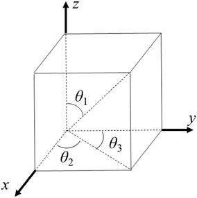
FIGURE 1. Schematic diagram in the rectangular coordinate system.

Based on the experimental measurements (Winkler and Liu, 1996) under the hydrostatic pressures for Portland sandstone, we calculate velocities for the longitudinal mode against pressure. The physical constants for the simulation are picked from Tables III-IV of (Winkler and Liu, 1996). The prestress condition in the simulation is regarded as the confining stress with its implementation described in detail in Section 4.1. The result is shown in Figure 2, where the circles (experimental measurements) are obtained by picking the pixel coordinates in Figure 4 of (Winkler and Liu, 1996). We see a weak nonlinearity for velocity variations with increasing pressures, resulting from the third-order elasticity with a cubic term for the strain energy function. Some departures from experimental measurements can be observed during the pressure of 20–60 MPa possibly because of the deformation of pores in the sandstone which the third-order elasticity for solids cannot account for. In general, for most consolidated rocks, the third-order elasticity could be enough to describe the nonlinear stress dependence of velocity variations.

FIGURE 2

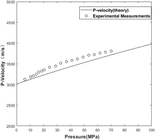
FIGURE 2. Velocities (solid line) of the longitudinal mode as a function of pressure based on the experimental measurements (circles) of hydrostatic pressure (Winkler and Liu, 1996) for Portland sandstone.

Numerical Methodolgy

Velocity–Stress Version of Acoustoelastic Equations for Space- and Time-Derivative Approximations

Equation 1 can be written as the first-order velocity-stress equation,

$\{\begin{array}{c}\rho v_{\beta ,t}={\tau }_{\alpha \beta ,\alpha },\\ {\tau }_{\alpha \beta ,t}=A_{\alpha \beta \gamma \delta }{v}_{\gamma ,\delta }\end{array}(22)$

where $v$ and $\tau$ are velocity and stress, respectively. With Eq. 11 and the Cartesian tensor notation with the x- and z-coordinates for convenience, we rewrite Eq. 22 as its velocity-stress FD formulation,

$\{\begin{array}{c}\rho v_{x,t}={\tau }_{xx,z}+{\tau }_{xz,z},\\ \rho v_{z,t}={\tau }_{xz,x}+{\tau }_{zz,z},\\ {\tau }_{xx,t}=A_{11}{v}_{x,x}+A_{13}{v}_{z,z}+A_{15}\left(v_{x,z}+v_{z,x}\right),\\ {\tau }_{zz,t}=A_{13}{v}_{x,x}+A_{33}{v}_{z,z}+A_{35}\left(v_{x,z}+v_{z,x}\right),\\ {\tau }_{xz,t}=A_{15}{v}_{x,x}+A_{35}{v}_{z,z}+A_{55}\left(v_{x,z}+v_{z,x}\right)\end{array}(23)$

The nonlinear effect of predeformation is introduced by the effective elastic constants. Equation 23 can be reduced to the classical elastic wave equation when no static stress is applied.

The SSG-FD method is widely used in seismology to simulate elastic wave propagation. The method defines velocity components, stress components, and physical properties in four grids crosswise shown in Figure 3A, whereas the RSG-FD method defines velocity components in one grid and stress components and elastic parameters in another grid shown in Figure 3B. The RSG-FD method is employed in this study to solve the first-order velocity-stress acoustoelastic equations.

FIGURE 3

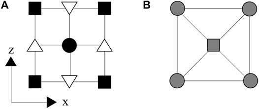
FIGURE 3. Schematic diagram of finite difference operators for SSG (A) and RSG (B). The SSG defines normal stress and all physical parameters in the solid squares, and shear stress in the solid circle, but with horizontal and vertical velocities in the downward and upward triangles, respectively. The RSG defines horizontal and vertical velocities in the square, but with normal and shear stresses and all physical parameters in the circles, where the line represents the direction of differentiation.

As shown in Figure 3B, the RSG technique calculates the spatial derivative along the diagonal direction of grids, and then interpolates the result along the normal coordinate axis to obtain the spatial derivative along the horizontal and vertical directions. We rotate the direction of spatial derivatives from the horizontal ($\mathrm{x}$) and vertical ($\mathrm{z}$) directions to the diagonal directions ($\overline{\mathrm{x}}$ and $\overline{\mathrm{z}}$) as

$\{\begin{array}{c}\overline{\mathbf{x}}=\frac{\Delta x}{\Delta r}\mathbf{x}-\frac{\Delta z}{\Delta r}\mathbf{z},\\ \overline{\mathbf{z}}=\frac{\Delta x}{\Delta r}\mathbf{x}+\frac{\Delta z}{\Delta r}\mathbf{z},\end{array}(24)$

where $\Delta r=\sqrt{\Delta x^2+\Delta z^2}$. The first-order spatial derivatives along the horizontal and vertical directions become,

$\{\begin{array}{c}\frac{\partial }{\partial x}=\frac{\Delta r}{2\Delta x}\left(\frac{\partial }{\partial \overline{z}}+\frac{\partial }{\partial \overline{x}}\right),\\ \frac{\partial }{\partial z}=\frac{\Delta r}{2\Delta z}\left(\frac{\partial }{\partial \overline{z}}-\frac{\partial }{\partial \overline{x}}\right).\end{array}(25)$

With Eq. 25, it is easy to define the differentiation operators $D_{\overline{x} }$ and $D_{\overline{z} }$, which implement the spatial derivatives along diagonal directions ($\overline{x}$ and $\overline{z}$) in the time domain (Saenger et al., 2000),

$\{\begin{array}{c}{D}_{\overline{x}}u\left(x,z,t\right)=\frac{1}{\Delta r}\left[u\left(x-\frac{\Delta x}{2},z+\frac{\Delta z}{2},t\right)-u\left(x+\frac{\Delta x}{2},z-\frac{\Delta z}{2},t\right)\right],\\ D_{\overline{z}}u\left(x,z,t\right)=\frac{1}{\Delta r}\left[u\left(x+\frac{\Delta x}{2},z+\frac{\Delta z}{2},t\right)-u\left(x-\frac{\Delta x}{2},z-\frac{\Delta z}{2},t\right)\right].\end{array}(26)$

With Eqs. 25, 26, the numerical differentiation operators are obtained that perform the spatial derivatives along the x and z directions in the rotated staggered grid by a linear combination of the derivatives along the $\overline{x}$ and $\overline{z}$ directions,

$\{\begin{array}{c}\frac{\partial }{\partial x}u\left(x,z,t\right)\approx \frac{\Delta r}{2\Delta z}\left(D_{\overline{x}}u\left(x,z,t\right)+D_{\overline{z}}u\left(x,z,t\right)\right),\\ \frac{\partial }{\partial z}u\left(x,z,t\right)\approx \frac{\Delta r}{2\Delta z}\left(D_{\overline{x}}u\left(x,z,t\right)-D_{\overline{z}}u\left(x,z,t\right)\right).\end{array}(27)$

A detailed process of the implementation of the RGS-FD scheme is addressed as follows.

By that analogy, we express the L-order RSG of each physical quantity in the discrete form as

$\begin{array}{l}{v}_{x,x}(x,z)\approx {\displaystyle \sum }_{l=1}^{L/2}\frac{c_n}{2\Delta x}\left\{v_x\left(x+\left(l-1/2\right)\Delta x,z+\left(l-1/2\right)\Delta z\right)+v_x\left(x+\left(l-1/2\right)\Delta x,z-\left(l-1/2\right)\Delta z\right)-v_x\left(x-\left(l-1/2\right)\Delta x,z-\left(l-1/2\right)\Delta z\right)-v_x\left(x-\left(l-1/2\right)\Delta x,z+\left(l-1/2\right)\Delta z\right)\right\}\\ v_{z,x}(x,z)\approx {\displaystyle \sum }_{l=1}^{L/2}\frac{c_n}{2\Delta x}\left\{v_z\left(x+\left(n-1/2\right)\Delta x,z+\left(n-1/2\right)\Delta z\right)+v_z\left(x+\left(n-1/2\right)\Delta x,z-\left(n-1/2\right)\Delta z\right)-v_z\left(x-\left(n-1/2\right)\Delta x,z-\left(n-1/2\right)\Delta z\right)-v_z\left(x-\left(n-1/2\right)\Delta x,z+\left(n-1/2\right)\Delta z\right)\right\}\\ v_{x,z}(x,z)\approx {\displaystyle \sum }_{l=1}^{L/2}\frac{c_n}{2\Delta z}\left\{v_x\left(x+\left(l-1/2\right)\Delta x,z+\left(l-1/2\right)\Delta z\right)-v_x\left(x+\left(l-1/2\right)\Delta x,z-\left(l-1/2\right)\Delta z\right)-v_x\left(x-\left(l-1/2\right)\Delta x,z-\left(l-1/2\right)\Delta z\right)+v_x\left(x-\left(l-1/2\right)\Delta x,z+\left(l-1/2\right)\Delta z\right)\right\}\\ v_{z,z}(x,z)\approx {\displaystyle \sum }_{l=1}^{L/2}\frac{c_n}{2\Delta z}\left\{v_z\left(x+\left(l-1/2\right)\Delta x,z+\left(l-1/2\right)\Delta z\right)-v_z\left(x+\left(l-1/2\right)\Delta x,z-\left(l-1/2\right)\Delta z\right)-v_z\left(x-\left(l-1/2\right)\Delta x,z-\left(l-1/2\right)\Delta z\right)+v_z\left(x-\left(l-1/2\right)\Delta x,z+\left(l-1/2\right)\Delta z\right)\right\}\\ {\tau }_{xx,x}\left(x+\Delta x/2,z+\Delta z/2\right)\approx {\displaystyle \sum }_{l=1}^{L/2}\frac{c_n}{2\Delta x}\left\{{\tau }_{xx}\left(x+l\Delta x,z+l\Delta z\right)+{\tau }_{xx}\left(x+l\Delta x,z-\left(l-1\right)\Delta z\right) -{\tau }_{xx}\left(x-l\Delta x,z-\left(l-1\right)\Delta z\right)-{\tau }_{xx}\left(x-l\Delta x,z+l\Delta z\right)\right\}\\ {\tau }_{xz,x}\left(x+\Delta x/2,z+\Delta z/2\right)\approx {\displaystyle \sum }_{l=1}^{L/2}\frac{c_n}{2\Delta x}\left\{{\tau }_{xz}\left(x+l\Delta x,z+l\Delta z\right)+{\tau }_{xz}\left(x+l\Delta x,z-\left(l-1\right)\Delta z\right) -{\tau }_{xz}\left(x-l\Delta x,z-\left(l-1\right)\Delta z\right)-{\tau }_{xz}\left(x-l\Delta x,z+l\Delta z\right)\right\}\\ {\tau }_{zz,x}\left(x+\Delta x/2,z+\Delta z/2\right)\approx {\displaystyle \sum }_{n=1}^{L/2}\frac{c_n}{2\Delta x}\left\{{\tau }_{zz}\left(x+n\Delta x,z+n\Delta z\right)+{\tau }_{zz}\left(x+n\Delta x,z-\left(n-1\right)\Delta z\right) -{\tau }_{zz}\left(x-n\Delta x,z-\left(n-1\right)\Delta z\right)-{\tau }_{zz}\left(x-n\Delta x,z+n\Delta z\right)\right\}\\ {\tau }_{xx,z}\left(x+\Delta x/2,z+\Delta z/2\right)\approx {\displaystyle \sum }_{n=1}^{L/2}\frac{c_n}{2\Delta z}\left\{{\tau }_{xx}\left(x+n\Delta x,z+n\Delta z\right)-{\tau }_{xx}\left(x+n\Delta x,z-\left(n-1\right)\Delta z\right) -{\tau }_{xx}\left(x-n\Delta x,z-\left(n-1\right)\Delta z\right)+{\tau }_{xx}\left(x-n\Delta x,z+n\Delta z\right)\right\}\\ {\tau }_{xz,z}\left(x+\Delta x/2,z+\Delta z/2\right)\approx {\displaystyle \sum }_{l=1}^{L/2}\frac{c_n}{2\Delta z}\left\{{\tau }_{xz}\left(x+l\Delta x,z+l\Delta z\right)-{\tau }_{xz}\left(x+l\Delta x,z-\left(l-1\right)\Delta z\right) -{\tau }_{xz}\left(x-l\Delta x,z-\left(l-1\right)\Delta z\right)+{\tau }_{xz}\left(x-l\Delta x,z+l\Delta z\right)\right\}\\ {\tau }_{zz,z}\left(x+\Delta x/2,z+\Delta z/2\right)\approx {\displaystyle \sum }_{l=1}^{L/2}\frac{c_n}{2\Delta z}\left\{{\tau }_{zz}\left(x+l\Delta x,z+l\Delta z\right)-{\tau }_{zz}\left(x+l\Delta x,z-\left(l-1\right)\Delta z\right) -{\tau }_{zz}\left(x-l\Delta x,z-\left(l-1\right)\Delta z\right)+{\tau }_{zz}\left(x-l\Delta x,z+l\Delta z\right)\right\}\end{array}(28)$

where the differential coefficients $c_l$ will be specified subsequently. For the time derivatives, we use the second-order FD approximation with $v_i\left(\left(l+1/2\right)\Delta t\right)=v_i^{l+1/2}$ for velocity, where $\Delta t$ is the time step.

Simultaneous Matrix Equations

Substituting Eq. 28 into (23) and adding a source field in the simulation, we obtain the discrete form of the first-order velocity-stress acoustoelastic equations,

$\{\begin{array}{c}{\dot{v}}_x=\left({\partial }_x{\tau }_{xx}+{\partial }_z{\tau }_{xz}-f_x\right)/\rho ,\\ {\dot{v}}_z=\left({\partial }_x{\tau }_{xz}+{\partial }_z{\tau }_{zz}-f_z\right)/\rho ,\\ {\dot{\tau }}_{xx}=A_{11}{\partial }_x{v}_x+A_{13}{\partial }_z{v}_z+A_{15}\left({\partial }_z{v}_x+{\partial }_x{v}_z\right)+{\dot{f}}_{xx},\\ {\dot{\tau }}_{zz}=A_{13}{\partial }_x{v}_x+A_{33}{\partial }_z{v}_z+A_{35}\left({\partial }_z{v}_x+{\partial }_x{v}_z\right)+{\dot{f}}_{zz},\\ {\dot{\tau }}_{xz}=A_{15}{\partial }_x{v}_x+A_{35}{\partial }_z{v}_z+A_{55}\left({\partial }_z{v}_x+{\partial }_x{v}_z\right)+{\dot{f}}_{xz},\end{array}(29)$

where the cap dot represents the first-order partial derivative of time, and $f$ denotes the components of the external body force. The set of equations can be combined into a matrix system as

$\dot{\mathrm{v}}+\mathbf{s}=\mathbf{Mv}(30)$

where the product $\mathbf{Mv}$ is given by

$\mathbf{Mv}=\left[\begin{array}{cc}\begin{array}{cc}\begin{array}{cc}\begin{array}{cc}\begin{array}{c}0\\ 0\\ A_{11}{\partial }_x+A_{15}{\partial }_z\\ A_{13}{\partial }_x+A_{35}{\partial }_z\\ A_{15}{\partial }_x+A_{55}{\partial }_z\end{array}& \begin{array}{c}0\\ 0\\ A_{13}{\partial }_z+A_{15}{\partial }_x\\ A_{33}{\partial }_z+A_{35}{\partial }_x\\ A_{35}{\partial }_z+A_{55}{\partial }_x\end{array}\end{array}& \begin{array}{c}{\partial }_x/\rho \\ 0\\ 0\\ 0\\ 0\end{array}\end{array}& \begin{array}{c}0\\ {\partial }_z/\rho \\ 0\\ 0\\ 0\end{array}\end{array}& \begin{array}{c}{\partial }_z/\rho \\ {\partial }_x/\rho \\ 0\\ 0\\ 0\end{array}\end{array}\right]\left[\begin{array}{c}{v}_x\\ v_z\\ {\tau }_{xx}\\ {\tau }_{zz}\\ {\tau }_{xz}\end{array}\right],(31)$

and the source vector is

$\mathbf{s}={\left[\begin{array}{cc}\begin{array}{cc}\begin{array}{cc}\begin{array}{cc}{f}_x/\rho & f_z\end{array}/\rho & {\dot{f}}_{xx}\end{array}& {\dot{f}}_{zz}\end{array}& {\dot{f}}_{xz}\end{array}\right]}^T(32)$

For the time integration from $t$ to $t+\Delta t$, with the discretizing time as $t=n\Delta t$, we have,

$\{\begin{array}{c}{v}_x^{n+1}=v_x^n+\Delta t\left({\partial }_x{\tau }_{xx}^n+{\partial }_z{\tau }_{xz}^n-f_x^n\right)/\rho ,\\ v_z^{n+1}=v_z^n+\Delta t\left({\partial }_x{\tau }_{xz}^n+{\partial }_z{\tau }_{zz}^n-f_z^n\right)/\rho ,\\ {\tau }_{xx}^{n+1}={\tau }_{xx}^n+\Delta t\left(A_{11}{\partial }_x{v}_x^n+A_{13}{\partial }_z{v}_z^n+A_{15}\left({\partial }_z{v}_x^n+{\partial }_x{v}_z^n\right)+f_{xx}^n\right),\\ {\tau }_{zz}^{n+1}={\tau }_{zz}^n+\Delta t\left(A_{13}{\partial }_x{v}_x^n+A_{33}{\partial }_z{v}_z^n+A_{35}\left({\partial }_z{v}_x^n+{\partial }_x{v}_z^n\right)+f_{zz}^n\right),\\ {\tau }_{xz}^{n+1}={\tau }_{xz}^n+\Delta t\left(A_{15}{\partial }_x{v}_x^n+A_{35}{\partial }_z{v}_z^n+A_{55}\left({\partial }_z{v}_x^n+{\partial }_x{v}_z^n\right)+f_{xz}^n\right).\end{array}(33)$

The set of Eq. 33 can be combined into a matrix system as. ${\mathbf{v}}^{\mathbf{n}+1}={\mathbf{M}}^{\mathit{n}}{\mathbf{v}}^{\mathit{n}}+{\mathbf{s}}^{\mathit{n}}.$

CPML Absorbing Boundary

The conventional PML absorption boundary is unable to handle the reflections (evanescent waves) at grazing incidences, especially for low-frequency components. The CPML absorption boundary improves the absorption effect of evanescent waves, with efficient computations by introducing auxiliary variables to avoid convolutional calculations that need to store past-time wavefields. The implementation of the CPML boundary does not need to split velocity and stress fields, and is easily incorporated into the RSG-FD program.

The CPML absorption boundary with the selection of parameters is detailed in Appendix. The algorithm is developed by modifying the complex coefficient $S_k$ and introducing the auxiliary variables $d_k$, ${\alpha }_k$, and ${\chi }_k$, where $d_k$ denotes the damping profile, and two real variables ${\chi }_k\ge 1$ and ${\alpha }_x\ge 0$. Substituting Eq. A4 into Eq. A2 yields,

$\partial {\tilde{x}}_k=\frac{1}{S_k}\partial x_k=\left[\frac{1}{{\chi }_k}-\frac{d_k}{{\chi }_k^2\left(i\omega +a_k+d_k/{\chi }_k\right)}\right]\partial x_k=\frac{1}{{\chi }_k}\partial x_k+{\tilde{\psi }}_k(34)$

where ${\tilde{\psi }}_k$ is a memory variable that can be rewritten as

$i\omega {\tilde{\psi }}_k+\left(a_k+\frac{d_k}{{\chi }_k}\right){\tilde{\psi }}_k=-\frac{d_k}{{\chi }_k^2}\partial x_k(35)$

Using an inverse Fourier transform to Eq. 35, we have,

$\frac{\partial {\psi }_k}{\partial t}+\left(a_k+\frac{d_k}{{\chi }_k}\right){\psi }_k=-\frac{d_k}{{\chi }_k^2}\partial x_k(36)$

where ${\psi }_k$ is the inverse of ${\tilde{\psi }}_k$. This equation has an iterative solution of the form,

${\psi }_k^n={\psi }_k^{n-1}{e}^{-\left(a_k+d_k/{\chi }_k\right)\Delta t}+\frac{d_k\partial x_k}{{\chi }_k\left(a_k{\chi }_k+d_k\right)}\left(e^{-\left(a_k+d_k/{\chi }_k\right)\Delta t}-1\right)(37)$

Equation 37 is derived simply by solving a first-order differential equation, leading to the same result in Komatitsch and Martin (2007) obtained by a recursive convolution method.

The CPML absorbing boundary for the first-order velocity-stress formulation of acoustoelastic equations can be implemented by 1) applying Eqs. 27–38 for the estimation of various memory variables in the rotated operators, 2) substituting these memory variables into Eq. 34 to obtain the spatial derivatives of all the field components in the stretched coordinates, and 3) substituting the resulting spatial derivatives into the velocity–stress formulas (Eq. 22) to yield the following C-PML formulation of acoustoelastic equations,

$\{\begin{array}{l}\rho {\dot{v}}_x=\frac{1}{{\chi }_x}{\partial }_x{\tau }_{xx}+{\psi }_{x,{\tau }_{xx}}+\frac{1}{{\chi }_z}{\partial }_z{\tau }_{xz}+{\psi }_{z,{\tau }_{xz}}\text{,}\\ \rho {\dot{v}}_z=\frac{1}{{\chi }_x}{\partial }_x{\tau }_{xz}+{\psi }_{x,{\tau }_{xz}}+\frac{1}{{\chi }_z}{\partial }_z{\tau }_{zz}+{\psi }_{z,{\tau }_{zz}},\\ {\dot{\tau }}_{xx}=A_{11}\left(\frac{1}{{\chi }_x}{\partial }_x{v}_x+{\psi }_{x,v_x}\right)+A_{13}\left(\frac{1}{{\chi }_x}{\partial }_z{v}_z+{\psi }_{z,v_z}\right)+A_{15}\left(\frac{1}{{\chi }_z}{\partial }_z{v}_x+{\psi }_{z,v_x}+\frac{1}{{\chi }_x}{\partial }_x{v}_z+{\psi }_{x,v_z}\right),\\ {\dot{\tau }}_{zz}=A_{13}\left(\frac{1}{{\chi }_x}{\partial }_x{v}_x+{\psi }_{x,v_x}\right)+A_{33}\left(\frac{1}{{\chi }_z}{\partial }_z{v}_z+{\psi }_{z,v_z}\right)+A_{35}\left(\frac{1}{{\chi }_z}{\partial }_z{v}_x+{\psi }_{z,v_x}+\frac{1}{{\chi }_x}{\partial }_x{v}_z+{\psi }_{x,v_z}\right),\\ {\dot{\tau }}_{xz}=A_{15}\left(\frac{1}{{\chi }_x}{\partial }_x{v}_x+{\psi }_{x,v_x}\right)+A_{35}\left(\frac{1}{{\chi }_z}{\partial }_z{v}_z+{\psi }_{z,v_z}\right)+A_{55}\left(\frac{1}{{\chi }_z}{\partial }_z{v}_x+{\psi }_{z,v_x}+\frac{1}{{\chi }_x}{\partial }_x{v}_z+{\psi }_{x,v_z}\right).\end{array}(38)$

Stability Analysis

The stability criterion for the velocity–stress RSG-FD operator with equal grid spacings can be generally expressed as the following inequality (Masson et al., 2006),

$\frac{\Delta t{V}_{\text{max}}}{\Delta r}\le C ,(39)$

with

$C=\frac{1}{\sqrt{D}{{\displaystyle \sum }}_{k=1}^n\left|c_n\right|} ,(40)$

where $V_{\text{max}}$ represents the maximum phase velocity in the medium, D represents the spatial dimension, and $c_n$ are the differential coefficients depending on the order of the spatial operator. For an eighth-order spatial and second-order temporal 2D FD operators with coefficients $c_1=\frac{1225}{1024}$, $c_2=-\frac{245}{3072}$, $c_3=\frac{49}{5120}$, and $c_4=-\frac{5}{7168}$, we can calculate $C$ = 0.5497.

Numerical dispersion is one of the main factors affecting the accuracy of the finite-difference method. To reduce the level of numerical dispersions in the RSG-FD method, a discretization interval should be selected to ensure a good number of grid points $n_{\lambda }$ per minimum wavelength, which is generally calculated by

$n_{\lambda }=\frac{V_{\text{min}}}{\Delta r{f}_{\text{max}}},(41)$

where $V_{\text{min}}$ is the minimum phase velocity and $f_{\text{max} }$ is the maximum frequency, usually taken as four times the center frequency of the source. Dispersion errors accumulate with increasing propagation distances, which can be reduced by refining grids. Numerical experiments by Chen et al. (2006) show that no less than 3 grid points per wavelength are required for the RSG eighth-order operator.

Numerical Examples

In this section, we calculate wavefield snapshots under various prestress conditions. The RSG-FD numerical method is applied to the first-order velocity-stress acoustoelastic equations. The effective second-order elastic constants, generally as shown in Eq. 11, can be further simplified in terms of prestressed conditions addressed as follows.

To simplify calculations, we set the y-direction of the model to infinity, so that the 3D case is simplified into a plane strain problem. Numerical examples are calculated using the properties from the Portland sandstone (807 × 807) mm with the bulk and shear moduli and density set to 9.7 GPa, 7.3 GPa, and 2,140 kg/m³ (Winkler and Liu, 1996), respectively. The third-order elastic constants (A, B, C) = (−1,122, −419, −340) GPa. The RSG-FD numerical simulation is conducted by the eighth-order spatial and second-order temporal FD operators. The source is a vertical force located at the center of the model domain with the time history,

$s\left(t\right)=\left(t-t_0\right)e^{-{\left[\pi f_0\left(t-t_0\right)\right]}^2},(42)$

where the central frequency $f_0$ = 1.42 MHz, and $t_0$ is a delay time. According to Eq. 35 where the maximum frequency f_max = 4f₀ and $n_{\lambda }=3$ (Chen et al., 2006), we obtain $V_{\text{min}}= 1704 \text{m}/\text{s}$ as the condition of stability. Generally, for a given frequency, we determine the maximum velocity of the medium $v_{\text{max}}$ at a maximum prestress 50 MPa, but with $v_{\text{min}}$ at 0 MPa. From the parameters listed above, we can obtain $v_{\text{max}}=v_P=$ 3,528 m/s at 50 MPa and $v_{\text{min}}=v_S$ = 1,848 m/s at 0 MPa, which enables a time step of 2⋅10^–7 s and a grid size of 10^–4 m to satisfy the condition of stability.

Acoustoelastic Simulation Under the Confining Prestress

For this case, the stress field is isotropic under the hydrostatic stress $P$, leading to the same stress and strain in all the directions. The principal strain components can be expressed as,

$\{\begin{array}{c}{e}_{11}=e_{33}=-\frac{P}{3K},\\ e_{13}=0.\end{array}(43)$

Substituting into Eq. 11 leads to a stiffness matrix

$\{\begin{array}{c}{A}_{11}=\lambda +2\mu +\left(2\lambda +4\mu +4C+8B+2A\right)\left(-P/3K\right),\\ A_{33}=\lambda +2\mu +\left(2\lambda +4\mu +4C+8B+2A\right)\left(-P/3K\right),\\ A_{55}=\mu +\left(2\mu +2B+A\right)\left(-P/3K\right),\\ A_{13}=\lambda +\left(2\lambda +4C+4B\right)\left(-P/3K\right),\\ A_{51}=0,\\ A_{53}=0.\end{array}(44)$

Wavefield snapshots are calculated with increasing hydrostatic stresses, as shown in Figure 4 for the x-component of the particle velocity at t = 0.12 ms. We see that the stress-induced velocity variations are isotropic, with the amplitude along the wavefront changing in accordance with the characteristics of a vertical force source. We calculate the theoretical wave velocity by Eqs. 20, 21. Figure 5 compares the theoretical and simulated wave velocities at the same angle but with different prestresses. Figure 6 compares the theoretical and calculated wave velocities under the same pressure (10 MPa) but with different directions. Both the theoretical and simulated wave velocities agree well under the different prestress conditions. These comparisons validate numerical simulations at least in travel time.

FIGURE 4

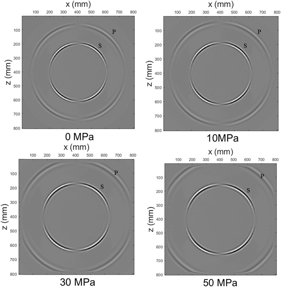
FIGURE 4. Wavefield snapshots of the x-component of the particle velocity at t = 0.12 ms for various hydrostatic stresses.

FIGURE 5

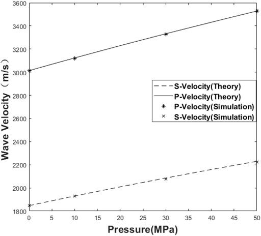
FIGURE 5. Comparison of the theoretical and calculated wave velocities for both the P-wave and S-wave as a function of hydrostatic prestresses (θ₁ = 0°).

FIGURE 6

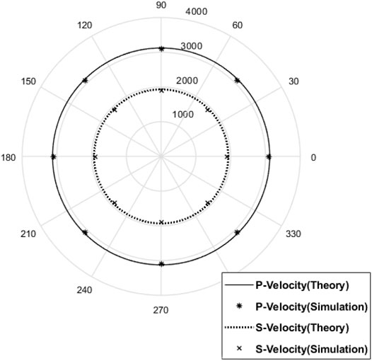
FIGURE 6. Comparison of the theoretical and calculated wave velocities for both the P-wave and S-wave under the same pressure (10 MPa) but with different directions.

Acoustoelastic Simulation Under the Uniaxial Prestress

For this case, the stress field is anisotropic under the uniaxial stress P. The principal strain components can be expressed as

$\{\begin{array}{c}{e}_{11}=\frac{P\left(\lambda +\mu \right)}{\mu \left(3\lambda +2\mu \right)},\\ e_{33}=-\frac{P\lambda }{2\mu \left(3\lambda +2\mu \right)},\\ e_{13}= 0.\end{array}(45)$

The corresponding stiffness matrix becomes,

$\{\begin{array}{c}{A}_{11}=\lambda +2\mu +\left(3\lambda +6\mu +2C+6B+2A\right)e_{11}+\left(2B+2C-\lambda -2\mu \right)e_{33},\\ A_{33}=\lambda +2\mu +\left(2B+2C-\lambda -2\mu \right)e_{11}+\left(6B+2C+2A+3\lambda +6\mu \right)e_{33},\\ A_{55}=\mu +\left(\mu +B+\frac{A}{2}\right)e_{11}+\left(\mu +B+\frac{A}{2}\right)e_{33},\\ A_{13}=\lambda +\left(\lambda +2C+2B\right)e_{11}+\left(2B+2C+\lambda \right)e_{33},\\ A_{51}=0,\\ A_{53}=0,\end{array}(46)$

Figure 7 shows the wavefield snapshots with increasing uniaxial stresses for the x-component of the particle velocity at t = 0.12 ms. With increasing uniaxial stresses, the P-wave and S-wave are gradually coupled together, with the wavefronts of qP-wave and qS-wave becoming more elliptical due to the stress-induced anisotropy of velocities. For p = 10 MPa, the qP-wave becomes elliptical slightly, but the qS-wave is almost a circle. For p = 30 MPa, we see a trigeminal region occurring symmetrically to connect the qS-wave and the qP-wave. The oval aspect ratio of the qP-wave becomes larger, implying an increasing velocity anisotropy on the longitudinal and transverse symmetry axes. For p = 50 MPa, we see more pronounced trigeminal region, approximately rhombic qS-wave, and elliptical qP-wave. Under the anisotropic predeformed condition, the polarization direction changes with the propagation direction, but neither parallel nor perpendicular to the propagation direction. These polarized waves are usually denoted by qP and qS, with their wavefronts deforming along the x-axis as the uniaxial stress increases. The azimuthal anisotropy of qP-wave is more and more obvious than that of the qS-wave, consistent with the mechanical mechanism of uniaxial stress. We calculate the principal strain direction according to Eq. 45 and mark it in the figure. It coincides with the directions of maximum/minimum velocities, which validates our numerical simulations. Thus, the directions of the velocity principal axis can indicate the directions of the principal strain for this case.

FIGURE 7

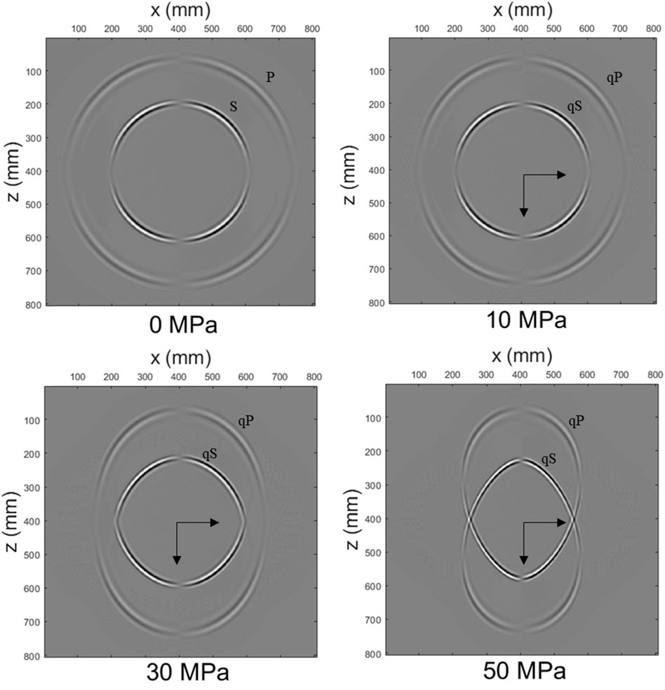
FIGURE 7. Wavefield snapshots of the x-component of the particle velocity at t = 0.12 ms for various uniaxial stresses. The arrow indicates the principal strain direction calculated by Eq. 45.

Acoustoelastic Simulation Under the Shear Prestress

As shown in Figure 8, the shear prestress can be classified into two cases: pure-shear and simple-shear deformations (Means and Williams, 1976). Different pre-deformations correspond to the different geological features. In order to identify these geological features in the seismic wave field, the simulations of pure shear and simple shear wavefield are carried out. For the former (see Figure 8A), the principal strain direction does not rotate with the progression of deformations, which is also called the non-rotational deformation or the coaxial deformation. In this case, the horizontal elongation and vertical contraction of deformations occur simultaneously under the uniaxial loading. The geological tensile and compressive effects produce a pure shear deformation.

FIGURE 8

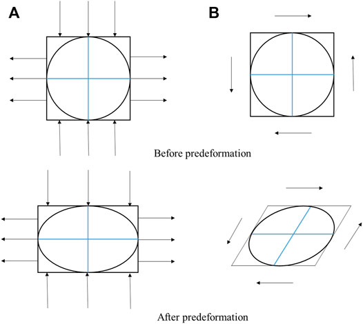
FIGURE 8. Schematic diagram of the deformation progression for pure (A) and simple (B) shear deformations.

The principal strain components for the pure-shear prestress become,

$\{\begin{array}{c}{e}_{11}=-e_{33}=\frac{P}{\lambda +2\mu },\\ e_{13}=0,\end{array}(47)$

yielding the following stiffness matrix,

$\{\begin{array}{c}{A}_{11}=\lambda +2\mu +\left(4\lambda +8\mu +4B-2A\right)e_{11 \mathrm{,}}\\ A_{33}=\lambda +2\mu -\left(4\lambda +8\mu +4B-2A\right)e_{11} ,\\ A_{55}=\mu ,\\ A_{13}=\lambda ,\\ A_{53}=0,\\ A_{51}=0.\end{array}(48)$

Wavefield snapshots are calculated with increasing pure-shear stresses and shown in Figure 9 for the x-component of the particle velocity at t = 0.12 ms. Similar to the case of uniaxial stresses, the circular wavefront at 0 MPa becomes more and more elliptical with increasing pure-shear stresses. The same changes in azimuthal anisotropy and amplitude can be seen as the uniaxial case. Unlike the uniaxial pressure condition, the absolute values of strains along the two axes of a pure-shear stress field are the same, implying that the stress-induced velocity anisotropy is more sensitive under the pure-shear prestress. Therefore, the velocities of qP-wave and qS-wave increase much more in the z-axis direction compared to the uniaxial case, as shown in Figure 7. We also calculate the principal strain direction according to Eq. 47 and mark it in the figure. It coincides with the directions of maximum/minimum velocities. Similarly, the directions of the velocity principal axis indicate the directions of the principal strain.

FIGURE 9

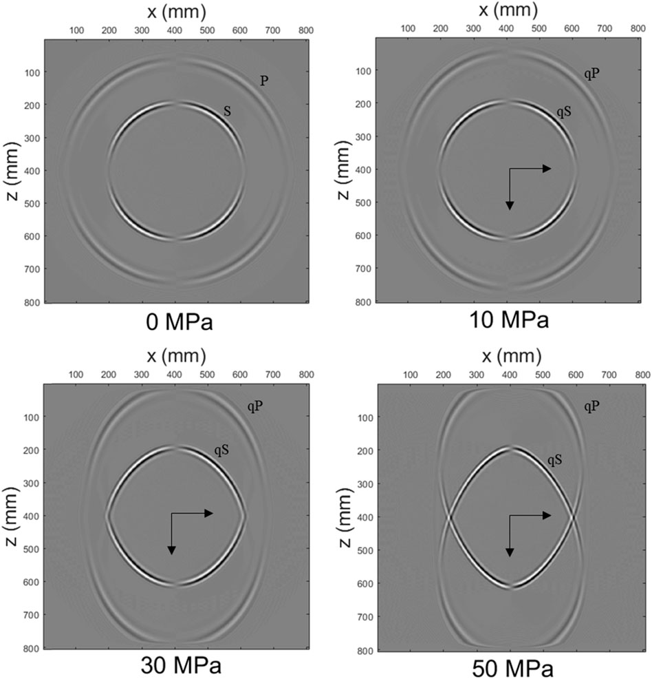
FIGURE 9. Wavefield snapshots of the x-component of the particle velocity at t = 0.12 ms for various pure-shear stresses. The arrow indicates the principal strain direction calculated by Eq. 47.

The deformation under the simple-shear prestress, as shown in Figure 8B, is rotational deformation or non-coaxial deformation. The direction and magnitude of two principal strains vary with increasing shear stresses, except for the strain parallel to the shear plane. Simple shear deformation is caused by shear sliding of a series of parallel sliding layers. For the simple-shear prestress, we have,

$\{\begin{array}{c}{e}_{13}=\frac{P}{\mu },\\ e_{11}=e_{33}=0,\end{array}(49)$

with the stiffness matrix as

$\{\begin{array}{c}{A}_{11}=\lambda +2\mu ,\\ A_{33}=\lambda +2\mu ,\\ A_{55}=\mu ,\\ A_{13}=\lambda ,\\ A_{53}=\left(2\lambda +4\mu +2B-A\right)e_{13},\\ A_{51}=\left(2\lambda +4\mu +2B-A\right)e_{13}.\end{array}(50)$

Wavefield snapshots are calculated with increasing shear stresses and shown in Figure 10 for the x-component of the particle velocity at t = 0.12 ms, respectively. We see that the wavefront characterizes the orientation of stresses. The stress-induced anisotropy becomes stronger with increasing stresses. Unlike the pure-shear stress loading, the axis of symmetry rotates in terms of stress orientations, which is consistent with the characteristics of shear stresses. The wavefronts of qP-wave and qS-wave become more elliptical and rotational with increasing shear stresses.

FIGURE 10

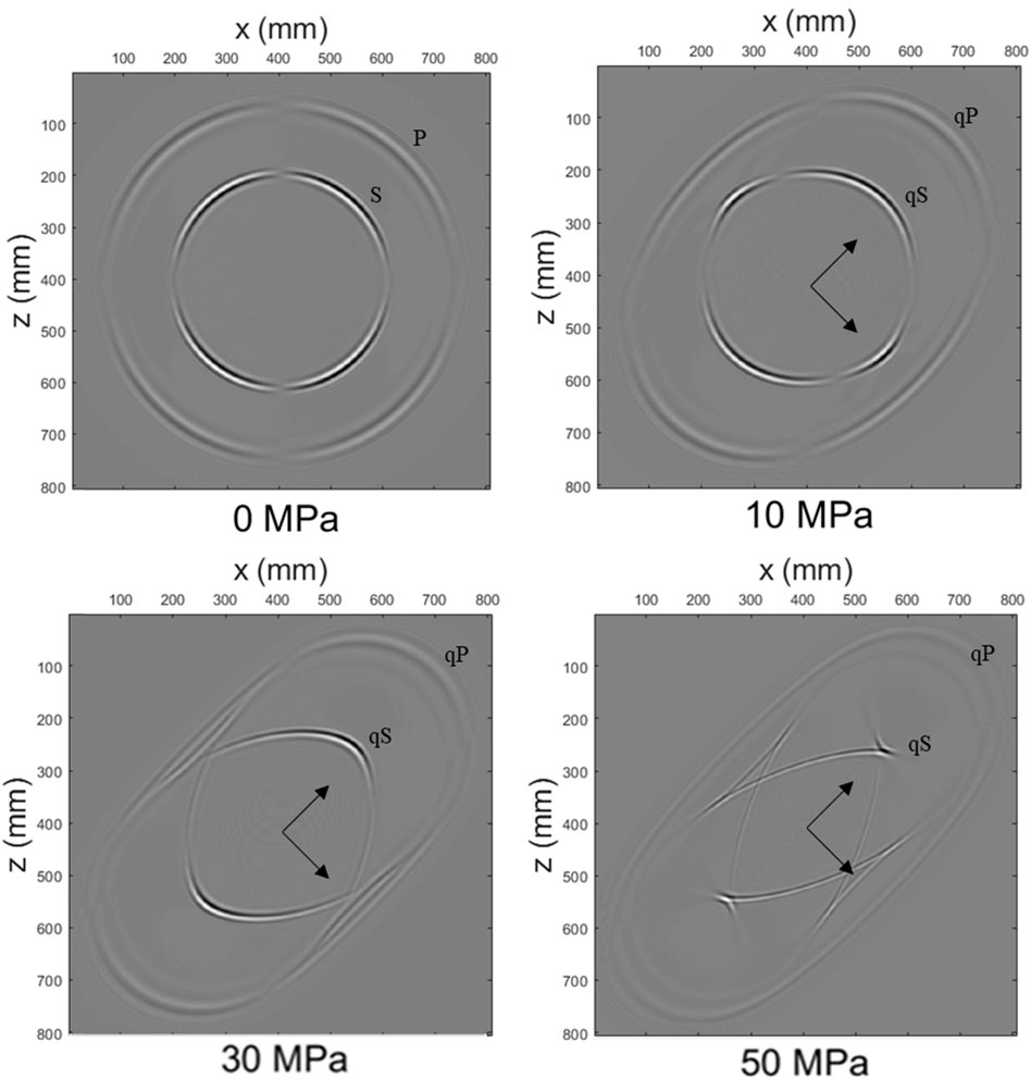
FIGURE 10. Wavefield snapshots of the x-component of the particle velocity at t = 0.12 ms for various simple shear stresses. The arrow indicates the principal strain direction calculated by Eq. 49.

To improve the understanding of the phenomenon observed in Figures 9, 10, we compare the changes in the P-wave velocity with θ₁ under both the pure-shear and simple-shear conditions, as shown in Figure 11. We see that the principal axis in the simple-shear case is shifted by about 45° relative to that in the pure-shear case, which is consistent with the direction by a shift of the principal strain axis. Therefore, the shift of the velocity principal axis direction can be used to judge the geological characteristics of the region.

FIGURE 11

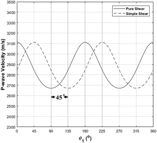
FIGURE 11. Variations of P-wave velocity against θ₁ under the pure-shear (solid line) and simple-shear (dashed line) conditions.

Acoustoelastic Simulation for a Double-Layer Model

The double-layer model, separated by a plane interface, is presented to investigate the reflection/transmission at the interface under the four different cases of loading prestress. The upper medium has the same properties as previous simulations. The lower medium has K = 5.6 GPa, μ = 2.3 GPa (A, B, C) = (-23, -10, -13) GPa, and ρ = 1,200 kg/m³. Consider an interface between two elastic media indicated by the + and - superscripts. The boundary condition at the interface requires the continuity of tractions and displacements. These conditions could be written as

$\{\begin{array}{c}{\tau }_{ij}^{+}{n}_j={\tau }_{ij}^{-}{n}_j,\\ u_i^{+}=u_i^{-},\end{array}(51)$

where $n_i$ represents the unit normal to the interface. Einstein’s summation convention for repeating indices is assumed.

Figure 12 shows the x-component of the particle velocity snapshots at t = 0.08 ms under four different prestress conditions: hydrostatic, uniaxial stress, pure-shear, and simple-shear stresses. The location of the source is marked by a star in Figure 12A. All the wave types of reflection/transmission can be observed from these snapshots which illustrate that the stress-induced velocity anisotropy is strongly related to the orientation of prestresses.

FIGURE 12

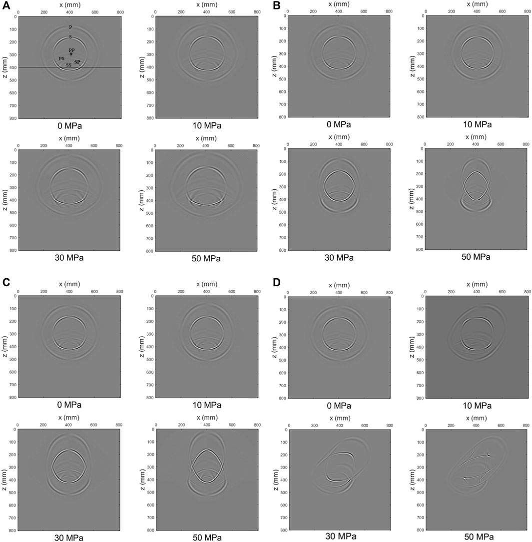
FIGURE 12. Wavefield snapshots of the x-component of velocity at t = 0.08 ms for a double-layer model under various hydrostatic stresses (A), uniaxial stresses (B), pure-shear stresses (C), and simple-shear stresses (D). The location of the source is marked by a star in the figure. The consecutive wavefronts include P-wave (P), S-wave (S), P-wave reflection (PP), S-wave reflection (SS), P-wave converted S-wave (PS), and S-wave converted P-wave (SP) are observed.

Conclusion

Acoustoelastic theory describes wave propagation in prestressed media and relates elastic wave velocities to prestresses, resulting from the third-order elasticity with a cubic term for the strain energy function. We propose an acoustoelastic modeling scheme for elastic wave propagation in prestressed media based on the RSG-FD method with the CPML absorbing boundary. The RSG-FD numerical method is applied to the first-order velocity-stress acoustoelastic equations. We address several aspects in the numerical implementation. Four states of prestress, confining-hydrostatic, uniaxial-stress, pure-shear, and simple-shear patterns, are investigated with different simplified stiffness matrices to model the prestress-induced anisotropy of velocities and its effect on the characteristics of wavefronts. The main conclusions can be summarized as follows.

1) A plane-wave analysis combined with closed-pore jacketed sandstone experiments illustrates the effect of third-order elastic constants on the P- and S-wave velocities under various prestresses. For most consolidated rocks, the third-order elasticity could be enough to describe the nonlinear stress dependence of velocity variations.

2) We partially validate the presented numerical scheme by the plane-wave theoretical solution. Comparisons between theoretical and calculated wave velocities are performed at the same angle but with different prestresses and under the same pressure (10 MPa) but with different directions, respectively.

3) Acoustoelastic simulations demonstrate that the confining prestress leads to the same stress and strain in all the directions, yielding isotropic velocity variations, whereas the uniaxial stress generates an anisotropic stress field, making the P-wave and S-wave be gradually coupled together, with the wavefronts of qP-wave and qS-wave becoming more elliptical due to the stress-induced anisotropy of velocities.

4) The pure-shear prestress with a coaxial deformation (horizontal elongation and vertical contraction) induces obvious elliptical wavefronts because of the stress-induced anisotropy of velocities that, unlike the uniaxial prestress, becomes more sensitive to the z-axis direction along which the velocities of qP-wave and qS-wave increase much more compared with the uniaxial case.

5) Unlike the pure-shear stress loading, the simple-shear prestress with a non-coaxial rotational deformation rotates the axis of symmetry in terms of stress orientations. The direction and magnitude of strains vary with increasing shear stresses, except for the strain parallel to the shear plane. The stress-induced anisotropy of velocities is sensitive to the orientation of stresses. the wavefronts of qP-wave and qS-wave become more elliptical and rotational with increasing shear stresses.

6) Numerical acoustoelastic simulations provide us with the possibility to explore wave propagation in deep high-pressure formations. However, the third-order elastic constants used are limited to isotropic solid media without microstructures. Considering that fractures are sensitive to prestress conditions, we will develop numerical schemes for anisotropic acoustoelastic equations of fractured media in the near future.

Data Availability Statement

The original contributions presented in the study are included in the article/Supplementary Material, further inquiries can be directed to the corresponding author.

Author Contributions

L-YF and HY conceive this research. HY writes the manuscript and prepares the figures. L-YF and B-YF reviews and supervises the manuscript. The coauthors TM are involved in the discussion of the manuscript. All authors finally approve the manuscript and thus agree to be accountable for this work.

Funding

The research was supported by the National Natural Science Foundation of China (Grant Nos. 41,821,002, 41,720,104,006).

Conflict of Interest

The authors declare that the research was conducted in the absence of any commercial or financial relationships that could be construed as a potential conflict of interest.

Publisher’s Note

All claims expressed in this article are solely those of the authors and do not necessarily represent those of their affiliated organizations, or those of the publisher, the editors and the reviewers. Any product that may be evaluated in this article, or claim that may be made by its manufacturer, is not guaranteed or endorsed by the publisher.

References

Alkhimenkov, Y., Räss, L., Khakimova, L., Quintal, B., and Podladchikov, Y. (2021). Resolving Wave Propagation in Anisotropic Poroelastic media Using Graphical Processing Units (GPUs). J. Geophys. Res. Solid Earth e2020JB021175. doi:10.1029/2020jb021175

CrossRef Full Text | Google Scholar

Carcione, J. M. (1999). Staggered Mesh for the Anisotropic and Viscoelastic Wave Equation. Geophysics 64, 1863–1866. doi:10.1190/1.1444692

CrossRef Full Text | Google Scholar

Carcione, J. M. (2007). Wavefields in Real Media: Wave Propagation in Anisotropic, Anelastic, Porous and Electromagnetic Media. 2nd Edn. Elsevier Science.

Google Scholar

Chen, H., Wang, X., and Lin, W. (2006). Parallel Numerical Simulation of the Ultrasonic Waves in a Prestressed Formation. Ultrasonics 44, e1013–e1017. doi:10.1016/j.ultras.2006.05.049

PubMed Abstract | CrossRef Full Text | Google Scholar

Crase, E. (1990). High-order (Space and Time) Finite-Difference Modeling of the Elastic Wave Equation. 60th Annu. Internat. Mtg., Soc. Expl. Geophys., Expanded Abstr. 90, 987

Google Scholar

Fang, X., Fehler, M., Zhu, Z., Chen, T., Brown, S., Cheng, A., et al. (2013). An Approach for Predicting Stress-Induced Anisotropy Around a Borehole. Geophysics 78, D143–D150. doi:10.1190/geo2012-0145.1

CrossRef Full Text | Google Scholar

Gao, K., and Huang, L. (2017). An Improved Rotated Staggered-Grid Finite-Difference Method with Fourth-Order Temporal Accuracy for Elastic-Wave Modeling in Anisotropic media. J. Comput. Phys. 350, 361–386. doi:10.1016/j.jcp.2017.08.053

CrossRef Full Text | Google Scholar

Goldberg, Z. A. (1961). Interaction of Plane Longitudinal and Transverse Elastic Waves. Sov. Phys. Acoust. 63, 306–310.

Google Scholar

Green, R. E. (1973). Ultrasonic Investigation of Mechanical Properties.” in Treatise on Materials Science and Technology, Vol. 3. New York: Academic Press.

Google Scholar

Gregor, D., Moczo, P., Kristek, J., Mesgouez, A., Lefeuve-Mesgouez, G., and Kristekova, M. (2021). Subcell-resolution Finite-Difference Modelling of Seismic Waves in Biot and JKD Poroelastic media. Geophys. J. Int. 224, 760. doi:10.1093/gji/ggaa454

CrossRef Full Text | Google Scholar

Hu, Y., and McMechan, G. (2010). Sensitivity of Three-Component 3D Finitedifference Elastic Seismic Modeling to Inclusion Parameters in HTI and TTI media with High Inclusion Density. Geophysics 75, 48–61. doi:10.1190/1.3358159

CrossRef Full Text | Google Scholar

Huang, X., Burns, D. R., and Toksöz, M. N. (2001). The Effect of Stresses on the Sound Velocity in Rocks: Theory of Acoustoelasticity and Experimental Measurements. Tech. Report. Boston: Earth Resources Laboratory, Massachusetts Institute of Technology.

Google Scholar

Johnson, P. A., and Shankland, T. J. (1989). Nonlinear Generation of Elastic Waves in Granite and sandstone: Continuous Wave and Travel Time Observations. J. Geophys. Res. 94, 17729–17733. doi:10.1029/jb094ib12p17729

CrossRef Full Text | Google Scholar

Komatitsch, D., and Martin, R. (2007). An Unsplit Convolutional Perfectly Matched Layer Improved at Grazing Incidence for the Seismic Wave Equation. Geophysics 72, SM155–SM167. doi:10.1190/1.2757586

CrossRef Full Text | Google Scholar

Li, Y., Liu, H., Wang, Y., Liu, Y., Liu, T., and Luo, Q. (2020). Acoustoelastic Effect Simulation by Time-Space Finite Element Formulation Based on Quadratic Interpolation of the Acceleration. Wave Motion 93, 102465. doi:10.1016/j.wavemoti.2019.102465

CrossRef Full Text | Google Scholar

Lisitsa, V., and Vishnevskiy, D. (2010). Lebedev Scheme for the Numerical Simulation of Wave Propagation in 3D Anisotropic Elasticity‡. Geophys. Prospecting 58, 619–635. doi:10.1111/j.1365-2478.2009.00862.x

CrossRef Full Text | Google Scholar

Liu, Q. H., and Sinha, B. K. (2000). Multipole Acoustic Waveforms in Fluid‐filled Boreholes in Biaxially Stressed Formations: A Finite‐difference Method. Geophysics 65, 190–201. doi:10.1190/1.1444710

CrossRef Full Text | Google Scholar

Lys, E., Romenski, E., Tcheverda, V., Epov, M., and Epov, M. I. (2015). “Finite-difference Simulation of Wave Propagation through Prestressed Elastic media,” in International Conference on Finite Difference Methods (Springer), 282–289. doi:10.1007/978-3-319-20239-6_30

CrossRef Full Text | Google Scholar

Martin, R., and Komatitsch, D. (2009). An Unsplit Convolutional Perfectly Matched Layer Technique Improved at Grazing Incidence for the Viscoelastic Wave Equation. Geophys. J. Int. 179, 333–344. doi:10.1111/j.1365-246x.2009.04278.x

CrossRef Full Text | Google Scholar

Masson, Y. J., Pride, S. R., and Nihei, K. T. (2006). Finite Difference Modeling of Biot's Poroelastic Equations at Seismic Frequencieserence Modeling of Biot’s Poroelastic Equations at Seismic Frequencies. J. Geophys. Res. 111, B10305. doi:10.1029/2006jb004366

CrossRef Full Text | Google Scholar

Mavko, G., Mukerji, T., and Godfrey, N. (1995). Predicting Stress‐induced Velocity Anisotropy in Rocks. Geophysics 60, 1081–1087. doi:10.1190/1.1443836

CrossRef Full Text | Google Scholar

Means, W. D., and Williams, P. F. (1976). An Outline of Structural Geology. John Wiley.

Google Scholar

Meegan, G. D., Johnson, P. A., Guyer, R. A., and McCall, K. R. (1993). Observations of Nonlinear Elastic Wave Behavior in sandstone. The J. Acoust. Soc. America 94, 3387–3391. doi:10.1121/1.407191

CrossRef Full Text | Google Scholar

Moczo, P., Gregor, D., Kristek, J., and de la Puente, J. (2019). A Discrete Representation of Material Heterogeneity for the Finite-Difference Modelling of Seismic Wave Propagation in a Poroelastic Medium. Geophys. J. Int. 216, 1072–1099. doi:10.1093/gji/ggy412

CrossRef Full Text | Google Scholar

Moczo, P., Kristek, J., Vavryčuk, V., Archuleta, R. J., and Halada, L. (2002). 3D Heterogeneous Staggered-Grid Finite-Difference Modeling of Seismic Motion with Volume Harmonic and Arithmetic Averaging of Elastic Moduli and Densities. Bull. Seismological Soc. America 92, 3042–3066. doi:10.1785/0120010167

CrossRef Full Text | Google Scholar

Norris, A. N. (1983). Propagation of Plane Waves in a Pre‐stressed Elastic Medium. J. Acoust. Soc. America 74, 1642–1643. doi:10.1121/1.390131

CrossRef Full Text | Google Scholar

Pao, Y.-H., Sachse, W., and Fukuoka, H. (1984). “Acoustoelasticity and Ultrasonic Measurements of Residual Stresses,”in Physical Acoustics, Principles and Methods. Editors W. P. Mason, and R. N. Thurston (Orlando: Academic Press), 17, 61–143.

Google Scholar

Pao, Y. H., and Gamer, U. (1985). Acoustoelastic Waves in Orthotropic media. J. Acoust. Soc. America 77, 806–812. doi:10.1121/1.392384

CrossRef Full Text | Google Scholar

Pau, A., and Vestroni, F. (2019). The Role of Material and Geometric Nonlinearities in Acoustoelasticity. Wave Motion 86, 79–90. doi:10.1016/j.wavemoti.2018.12.005

CrossRef Full Text | Google Scholar

Pei, Z., Fu, L.-Y., Sun, W., Jiang, T., and Zhou, B. (2012). Anisotropic Finite-Difference Algorithm for Modeling Elastic Wave Propagation in Fractured Coalbeds. Geophysics 77, C13–C26. doi:10.1190/geo2010-0240.1

CrossRef Full Text | Google Scholar

Saenger, E. H., and Bohlen, T. (2004). Finite‐difference Modeling of Viscoelastic and Anisotropic Wave Propagation Using the Rotated Staggered Grid. Geophysics 69, 583–591. doi:10.1190/1.1707078

CrossRef Full Text | Google Scholar

Saenger, E. H., Gold, N., and Shapiro, S. A. (2000). Modeling the Propagation of Elastic Waves Using a Modified Finite-Difference Grid. Wave Motion 31, 77–92. doi:10.1016/s0165-2125(99)00023-2

CrossRef Full Text | Google Scholar

Saenger, E. H., and Shapiro, S. A. (2002). Effective Velocities in Fractured media: a Numerical Study Using the Rotated Staggered Finite-Difference Grid. Geophys. Prospect. 50, 183–194. doi:10.1046/j.1365-2478.2002.00309.x

CrossRef Full Text | Google Scholar

Seron, F. J., Badal, J., and Sabadell, F. J. (1996). A Numerical Laboratory for Simulation and Visualization of Seismic Wavefields1. Geophys. Prospect. 44, 603–642. doi:10.1111/j.1365-2478.1996.tb00168.x

CrossRef Full Text | Google Scholar

Shams, M., Destrade, M., and Ogden, R. W. (2011). Initial Stresses in Elastic Solids: Constitutive Laws and Acoustoelasticity. Wave Motion 48, 552–567. doi:10.1016/j.wavemoti.2011.04.004

CrossRef Full Text | Google Scholar

Sinha, B. K., and Kostek, S. (1996). Stress‐induced Azimuthal Anisotropy in Borehole Flexural Waves. Geophysics 61, 1899–1907. doi:10.1190/1.1444105

CrossRef Full Text | Google Scholar

Thurston, R. N., and Brugger, K. (1964). Third-order Elastic Constants and the Velocity of Small Amplitude Elastic Waves in Homogeneously Stressed media. Phys. Rev. 133, 1604–1610. doi:10.1103/physrev.133.a1604

CrossRef Full Text | Google Scholar

Toupin, R. A., and Bernstein, B. (1961). Sound Waves in Deformed Perfectly Elastic Materials. Acoustoelastic Effect. J. Acoust. Soc. America 33, 216–225. doi:10.1121/1.1908623

CrossRef Full Text | Google Scholar

Virieux, J. (1986). P-SV Wave Propagation in Heterogeneous media: Velocity‐stress Finite‐difference Method. Geophysics 51, 889–901. doi:10.1190/1.1442147

CrossRef Full Text | Google Scholar

Winkler, K. W., and Liu, X. (1996). Measurements of Third‐order Elastic Constants in Rocks. J. Acoust. Soc. America 100, 1392–1398. doi:10.1121/1.415986

CrossRef Full Text | Google Scholar

Yang, Y., Ng, C. T., Mohabuth, M., and Kotousov, A. (2019). Finite Element Prediction of Acoustoelastic Effect Associated with Lamb Wave Propagation in Pre-stressed Plates. Smart Mater. Struct. 28, 095007. doi:10.1088/1361-665x/ab2dd3

CrossRef Full Text | Google Scholar

Zhang, Y., Fu, L.-Y., Zhang, L., Wei, W., and Guan, X. (2014). Finite Difference Modeling of Ultrasonic Propagation (Coda Waves) in Digital Porous Cores with Un-split Convolutional PML and Rotated Staggered Grid. J. Appl. Geophys. 104, 75–89. doi:10.1016/j.jappgeo.2014.02.012

CrossRef Full Text | Google Scholar

Zong, J. (2014). Elastic Properties of Salt: Laboratory Measurements, Well-Log Analysis, and a Seismic Survey over the Hockley Salt Mine, Texas. Master Thesis. Texas: University of Houston.

Google Scholar

CPML Absorbing Boundary

This appendix summarizes the CPML absorption boundary (Komatitsch and Martin, 2007; Martin and Komatitsch, 2009). The conventional PML absorption boundary formulates various memory variables in the FD operator from the Cartesian coordinate to the complex coordinate by introducing a complex factor

$\tilde{x}=x-\frac{i}{\omega }{\int }_0^x{d}_x\left(s\right)ds,(\mathrm{A1})$

where i = $\sqrt{-1}$ and ω is the angular frequency. The damping factor $d_x\left(s\right)=$ 0 inside the computational domain and $d_x\left(s\right)$ > 0 in the PML region. The regular coordinate variable x is replaced by the complex coordinate variable $\tilde{x}$, with the corresponding differential operator as

${\partial }_{\tilde{x}}=\frac{1}{S_x}{\partial }_{x },(\mathrm{A2})$

where

$S_x=\frac{i\omega +d_x}{i\omega }=1+\frac{d_x}{i\omega } .(\mathrm{A3})$

The PML formulation is implemented directly by changing original wave equations written in terms of the variable x into new equations in terms of the variable $\tilde{x}$.

The conventional PML absorption boundary suffers from poor accuracy at grazing incidences. It also requires much memory and computation. The problem is related to the complex coefficient $S_{x }$ in Eq. A3. The CPML approach improves the performance of the PML by introducing two auxiliary variables, ${\alpha }_x$ and ${\chi }_x$. The modified complex coefficient becomes

$S_x={\chi }_x+\frac{d_x}{{\alpha }_x+i\omega } ,(\mathrm{A4})$

where ${\chi }_x\ge 1$ and ${\alpha }_x\ge 0$.

The CPML absorption boundary involves a number of absorption parameters. The maximum damping factor is usually set as

$d_{\text{max}}=-\frac{\left(m+1\right)V_{\text{max}}}{2L}\ln \left(R\right) ,(\mathrm{A5})$

where $V_{\text{max}}$ is the maximum phase velocity in the medium, L is the thickness of the absorption boundary layer, R is the theoretical reflection coefficient, and $m$ is the order of the polynomial (typically 2 or 3). The damping factor can be determined by

$d_x\left(l\right)=d_{\text{max}}{\left(\frac{l}{L}\right)}^m,(\mathrm{A6})$

where $l(0\le l\le L)$ is the distance from the calculated point to the boundary. The other parameters are accordingly set as

${\chi }_x=1+\left({\chi }_{\text{max}}-1\right){\left(\frac{l}{L}\right)}^m,(\mathrm{A7})$

and

${\alpha }_x=\pi \left(1-\frac{l}{L}\right){\alpha }_{\text{max}}(\mathrm{A8})$

The auxiliary variable ${\alpha }_x$ varies linearly between 0 and ${\alpha }_{\text{max}}$ in the absorption region. We usually take ${\alpha }_{\text{max}}=f_{0 }$ with $f_{0 }$ the main frequency of the source. For ${\alpha }_{\text{max}}=0$ and ${\chi }_x=1$, $S_{x }$ is reduced to that of the conventional PML boundary.