Data assimilation, sensitivity analysis and uncertainty quantification in semi-arid terminal catchments subject to long-term rainfall decline

Quantification of long-term hydrologic change in groundwater often requires the comparison of states pre- and post-change. The assessment of these changes in ungauged catchments using numerical models and other quantitative methods is particularly difficult from a conceptual point of view and due to parameter non-uniqueness and associated uncertainty of quantitative frameworks. In these contexts, the use of data assimilation, sensitivity analysis and uncertainty quantification techniques are critical to maximize the use of available data both in terms of conceptualization and quantification. This paper summarizes findings of a study undertaken in the Lake Muir-Unicup Natural Diversity Recovery Catchment (MUNDRC), a small-scale endorheic basin located in southwestern Australia that has been subject to a systematic decline in rainfall rates since 1970s. A combination of data assimilation techniques was applied to conceptual and numerical frameworks in order to understand and quantify impacts of rainfall decline on the catchment using a variety of metrics involving groundwater and lake levels, as well as fluxes between these compartments and mass balance components. Conceptualization was facilitated with the use of a novel data-driven method relating rainfall and groundwater responses running backwards in time, allowing the establishment of the likely baseline conditions prior to rainfall decline, estimation of net recharge rates and providing initial heads for the forward numerical modelling. Numerical model parameter and predictive uncertainties associated with data gaps were then minimized and quantified utilizing an Iterative Ensemble Smoother algorithm, while further refinement of conceptual model was made possible following results from sensitivity analysis, where major parameter controls on groundwater levels and other predictions of interest were quantified. The combination of methods can be considered as a template for other long-term catchment modelling studies that seek to constrain uncertainty in situations with sparse data availability.

1 Introduction

Endorheic basins, also known as terminal catchments of internally drained basins, comprise a variety of geomorphic environments widely distributed across the globe. These environments with often distinct attributes are characterized by the lack of surface and groundwater discharge across their borders and have evaporation as the dominant outflow. Despite many of them being currently under pressure from climate change and anthropogenic activities, these basins are understudied when compared to traditional hillslope catchments. The unique surface and groundwater attributes (De Sousa, 2021) of these environments makes extrapolations and inferences from better studied hillslope catchments difficult. From a quantitative perspective, modelling efforts in these areas are not only difficult given the lack of numerical frameworks designed for surface-groundwater interactions in semi-arid settings (Jolly et al., 2008), but they also suffer from a lack of site-specific monitoring data.

The issue of data sparsity is a common theme in endorheic basins, evidenced by the fact that current literature relies heavily on indirect measurements and remote-sensing data (De Sousa, 2021). Data sparsity hinders the ability to establish a robust conceptualization and incurs large predictive uncertainty which is inherent to surface and groundwater models. The need to maximize the extraction of information from largely incomplete datasets and its use in conceptualization and numerical modelling is critical for the development of quantitative frameworks that are capable of accounting for hydrogeological/hydrological uncertainty and the ability of available data to constrain it.

The use of Data Assimilation (DA), Uncertainty Quantification (UQ) and Sensitivity Analysis (SA) techniques in hydrological modelling is an emerging field with great potential to support decision-making in catchments experiencing hydrological change, but to date many of these techniques have not yet been applied to endorheic basin studies. Challenges remain on how to apply them appropriately in situations where the observation data is less than ideal, such that they can output useful information relevant to inform our conceptualization and strategies for management (Thompson et al., 2015).

Research into DA was initially developed for the purpose of numerical weather prediction, and is often related to Kalman filter contexts, where the states of variables from numerical models are updated incrementally through time as new observation data becomes available. In this paper, we adopt a broader definition of DA, which relates to optimally combine observations with theory (usually as numerical models) to improve model integrity and the accuracy of predictions of interest (Asch et al., 2016). In this regard, DA techniques are used for several purposes, such as history matching and parameter optimization based on observed data, determination of initial conditions for a numerical forecast model, interpolation of sparse observation datasets using the physical knowledge of the system (i.e., numerical models), and reduction of predictive uncertainty of numerical models.

The use of UQ and SA techniques is often interrelated with DA techniques. While UQ tends to focus on quantifying and reducing parameter and predictive uncertainty due to lack of data or model defects, SA looks at the effect that model parameters have on outputs of interest (Pianosi et al., 2016). These techniques have the potential to support many of the questions that arise from investigation efforts in endorheic basins, from conceptualization to quantification, predictive modeling, and adaptive management (Figure 1), which are explored next.

FIGURE 1

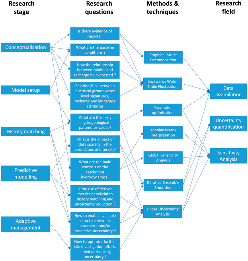
FIGURE 1. Example of DA, UQ and SA techniques, and their potential to support research in endorheic basins.

1.1 Finding evidence of long-term groundwater trends and reconstruction of baseline conditions

The use of signal analysis techniques for processing of time series and extraction of useful information is an import area of signal processing and well-established techniques such as Fourier Transforms and Wavelets have been applied for decades (Maheshwari and Kumar, 2014). Studies focused on groundwater level time series analysis include works by Lafare et al. (2016) and Seeboonruang (2014).

In situations where long-term stressors are intermixed with short-term signals (such as seasonality), time decomposition techniques have the potential to untangle them. The Empirical Model Decomposition method developed by Huang et al. (1998) is a technique for processing of non-linear and non-stationary signals and/or time series, decomposing them into a number of zero-mean signals called Intrinsic Mode Functions (IMF) in an adaptive and fully data-driven way, from the assumption that any signal is composed by different IMF’s and that each IMF represents a characteristic oscillation on a separated time scale. The EMD technique have been used in the hydrology field for identification of trends in lake levels (Wang et al., 2020) and groundwater forecasting (Gong et al., 2018).

Another challenge in the study of endorheic basins under long-term impacts is the establishment of pre-impact baseline conditions. For impact assessment in general, the definition of impacts often involves comparison of current and past hydrologic states. The absence of baseline data in these circumstances makes the definition of these impacts difficult both in terms of conceptualization and quantification. The Backward Water Table Fluctuation (BWTF) developed by De Sousa (2021) is a data-driven hindcasting technique based on rainfall and groundwater level fluctuations, enabling the reconstruction of baseline groundwater levels for periods where no monitoring data was available.

1.2 Data sparsity and uncertainty

Data sparsity in the endorheic basins reduces the reliability of investigation efforts, both in terms of identification of dominant processes (conceptualization) and predictive ability of quantitative frameworks.

More conventional applications of data assimilation involve the use of history-matching techniques to attempt the reduction of parameter uncertainty (and possibly predictive uncertainty). Excellent discussions on history-matching, data assimilation and their value in the reduction of uncertainty are presented by Nicols and Doherty (2020) and Gallagher and Doherty (2020). In these discussions, history matching is defined as the “act of tuning model parameters so that a model can reproduce past system behavior.” Predictive uncertainty in hydrologic models is often expressed from a conceptual point of view using Bayes equation, where imposition of constraints on parameter values is obtained through history-matching. Where approximations of prior distributions are derived from the conceptual understanding and expert-knowledge of a system (also known as soft-data), history-matching against field measurements (hard-data) induce alterations to the prior parameter probability distributions and, consequently, predictive uncertainty. The resulting probability distribution from parameter sets that both conform with expert-knowledge and reproduce historical behavior approximates the posterior probability distribution.

As discussed in Nicols and Doherty (2020), mathematical expressions for posterior parameter and predictive probability distribution cannot be derived, however, they can be defined by sampling them. The PESTPP-IES iterative ensemble smoother (White, 2018) was designed to this end. Based on the algorithm described by Chen and Oliver (2013), PESTPP-IES uses ensemble realizations derived from an approximation of the prior parameter probability distribution and attempt to adjust them by the minimum amount required to match field observations and achieve history-matching as well as reduction in parameter uncertainty.

1.3 Maximizing the use of available data sets with derived metrics

In the “Concept-State-Process-System” (CSPS) framework introduced for the hierarchical assessment of aquatic ecosystem models, Hipsey et al. (2020) divides metrics used for history matching of model states into 3 major groups: 1—Direct comparison, where model results are compared with measured data at specific points in time and space; 2—Derived metrics describing model state, which do not involve a direct assessment of a state variable, but are derived from them (such as head differences, or ratios between variables); and 3—Metrics describing multi-scale variability in model state, used to describe how well the various scales of spatial or temporal variability are described in models.

The use of derived metrics involving groundwater head differences in space and time is not new in hydrogeology studies and is recommended by several authors (Hill and Tiedeman, 2007; Doherty et al., 2010). Nevertheless, studies demonstrating and evaluating the value of derived metrics and how they contribute to reducing uncertainty is not often seen in literature.

1.4 Informing conceptualization and controls on catchment dynamics

Thompson et al. (2015) states that numerical models are important in understanding how complex catchment systems are responding to uncertain changes and while conceptual models usually guide the development of numerical models, iterative cycles between conceptualization and modelling results may be beneficial to refine conceptual understanding.

Saltelli et al. (2004) defines sensitivity analysis as “The study of how uncertainty in the output of a model (numerical or otherwise) can be apportioned to different sources of uncertainty in the model input.” In groundwater modelling practice, the sensitivity analysis is usually performed at the end of the modelling exercise, or as a by-product of parameter optimization methods used for history matching such as PEST (Doherty, 2015) and PESTPP (Welter et al., 2015). However, much can be gained from sensitivity analysis in terms of conceptualization if these techniques are employed in earlier stages of model development. Despite the fact that sensitivity can be anticipated to some extent by experienced modelers, rigorous analysis is useful to corroborate, indicate the need for new conceptualization, or diagnose non-linear behavior of models and/or numerical instabilities.

Algorithms based on the Gauss-Levemberg-Marquadt method such as PEST (Doherty, 2015, 2020), PESTPP (Welter et al., 2015) often require a tangent linear operator, also known as Jacobian matrix. These matrices contain partial derivatives of model outputs in respect to model parameters and are often required for history matching methods, sensitivity, and linear uncertainty analysis. Detailed analysis of these sensitive matrices can provide valuable insights on system functioning and dominant controls on catchment dynamics (as explored in the following sections). However, they are not often “dissected” and interpreted in context of model conceptualization.

While point-source sensitivities obtained from perturbation methods (such as those obtained by PEST and PESTPP) provide valuable insights on system and model behavior, there are situations where more robust sensitivity estimates are required. For these purposes, the use of global sensitivity analysis (GSA) may be useful. GSA methods characterize the effect of model parameter onto model outputs over a wide range of acceptable parameter values, covering larger portions of parameter space as opposed to point-source sensitivity. As a result, the behavior of model outputs that are non-linear and dependent on the combination of many parameters can be unraveled. Several methods for global sensitivity analysis with different degrees of computational effort and output results, as discussed in Saltelli et al. (2004, 2008).

1.5 Optimizing site investigation efforts

In data-scarce areas and resource-constrained investigations, it is important to collect data where it really matters. From a quantitative perspective, that means where and when an observation will promote the maximum reduction of predictive uncertainty. When a Jacobian sensitivity matrix is calculated for a parameter set that reasonably conforms with expert-knowledge and historical system behavior, it can be used for linear uncertainty analysis, also known as first-order second moment (FOSM) analysis. The theory behind linear uncertainty analysis is widely discussed in the literature (Moore and Doherty, 2006; James et al., 2009; Dausman et al., 2010; White et al., 2014) and it has been implemented in a number of model-independent software packages, including PEST, PESTPP and PyEMU (White et al., 2016).

This method provides an approximate mathematical characterization of prior and posterior probability distributions for parameters and predictions of interest (Nicols and Doherty, 2020). Furthermore, it can be used to demonstrate the value of history matching data (existing or not) in the reduction of parameter and predictive uncertainty. This enables the assessment of data worth not only for different data metrics, but also optimizing data acquisition efforts, by pre-empting its ability to constrain parameter and predictive uncertainty.

1.6 Study objectives and structure

The objective of this study is to apply and demonstrate the use of DA, UQ and SA techniques in the context of endorheic basins research, evaluating the ability of these methods to facilitate and enable conceptualization, quantification, and adaptive management measures. These techniques were applied during research undertaken at the Lake Muir-Unicup Natural Diversity Recovery Catchment (MUNDRC), a small scale semi-arid basin located in southwestern Australia, and subject to a systematic decline in rainfall rates over the past 50 years.

The application of the different techniques presented in this paper was not linear, in the sense they were not necessarily applied in the order they are presented. Multiple feedback loops between assessment of model results and conceptualization were undertaken, evolving the understanding of the site and robustness of quantitative assessments to the final form. The last part of this paper integrates the findings of all techniques and how they contributed to the research development.

2 Study site, conceptual and numerical framework

The area of investigation employed in this study is the Lake Muir-Unicup Natural Diversity Recovery Catchment (MUNDRC), located in southwestern Australia and listed under the Ramsar Convention as a Wetland of International Importance. This area consists of a complex system of lakes, swamps and flood plains, encompassing an area of 630 km² and is located 65 km from the coastline (Figure 2).

FIGURE 2

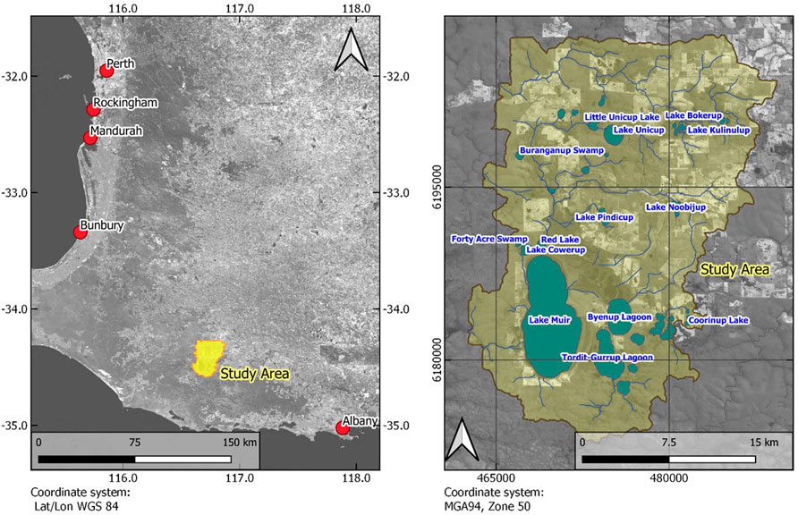
FIGURE 2. Location of study site, Lake Muir and nearby surface water compartments.

The conceptual model for the area, main hydrological drivers and effects from rainfall decline on surface and groundwater compartments are discussed in De Sousa (2021). Four hydrogeological units are associated with unconsolidated sediments and weathered portions of the crystalline basement. The combination of low relief, high specific yield, and flat lake bathymetry results in a relatively stagnant groundwater system with respect to horizontal flows along the lower plains surrounding Lake Muir. The flat topography also results in poor development of surface drainage lines, favoring infiltration processes over runoff, as well as the development of shallow groundwater tables with high correlation to the topography and significant seasonal oscillations.

Lake Muir is positioned in the lowest topographical area of the catchment and constitutes the largest groundwater discharge area, where water is constantly removed from the lake through evaporation. Water exchanges between the lake and adjacent aquifers is dynamic given the highly variable lake-aquifer interface areas resulting from the flat lakebed geometry.

Long-term rainfall records for the catchment show a systematic decrease in rainfall rates, particularly during the wet seasons. Hope and Foster (2005) analyzed winter rainfall rates in Western Australia for the period of 1925–2005 and identified an abrupt change in rainfall rates since 1970s.

Cumulative rainfall reductions for the MUNDRC have been undertaken using Accumulation Monthly Residual Rainfall (Ferdowsian et al., 2001) and are displayed in Figure 3, showing relatively small departures for the period from 1920–1970, with a pronounced negative departure from 1970 to present, showing a total deficit of 5,500 mm over 46 years. This reduction in rainfall results in smaller groundwater recharge and, consequently, reductions in groundwater levels and discharge volumes.

FIGURE 3

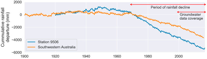
FIGURE 3. Cumulative rainfall departure for Station 9,506 and average southwestern Australia, using rainfall averages for the period of 1900–1970.

2.1 Numerical framework

A numerical framework for quantification of long-term impacts associated with rainfall decline on MUNDRC have been developed and described by De Sousa (2021). Aiming at representing the main hydrologic controls in the area and encapsulating both conceptualization and monitoring data, the framework consisted of a dynamically-coupled lake and groundwater model, accompanied by a rainfall-based groundwater recharge formulation.

The three-dimensional groundwater model was built using the finite element code FEFLOW (Diersch, 2014), coupled with a lake model component developed using FEFLOW’s API. The model was defined based on catchment boundaries and geometry of the main hydrogeological units in the area (Figure 4).

FIGURE 4

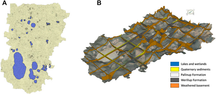
FIGURE 4. Groundwater model mesh and main surface water compartments (A), and fence diagram illustrating the distribution of the main hydrogeological units (B).

The model was initially calibrated against lake and groundwater levels, as well as additional derived metrics discussed later in the section below, using piecewise-constant parameter zones, where hydrogeological parameters of the different aquifers were assumed to be homogeneous over their extent.

This numerical framework was upgraded in this paper by adopting a highly-parameterized approach using pilot points (Doherty et al., 2010). The use of pilot points not only allows for heterogeneity within the aquifers, but also builds the foundation for the DA, UQ and SA workflows presented in this paper. Pilot points were assigned covering the extent of each of the aquifer and recharge zones, using a predominantly regular grid with 1,500 m spacing (Figure 5). Each aquifer pilot point was assigned four parameters and two parameters were assigned for each recharge pilot point. Three additional parameters were also implemented to define initial lake level and multipliers for lake evaporation and rainfall, resulting in 3,295 parameters adjusted during history matching and analyzed in the uncertainty quantification and sensitivity analyses (Table 1). In order to facilitate the discussion, the following convention was used for parameter naming:

FIGURE 5

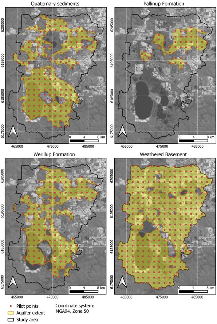
FIGURE 5. Distribution of pilot points for the different hydrogeological units.

TABLE 1

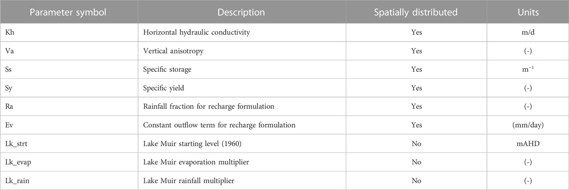
TABLE 1. Parameter type descriptors used in parameter name definition.

Ptype _Pzone _PPID

where Ptype is the type of parameter, Pzone relates to the original parameter zones defined De Sousa (2021) and PPID correspond to the pilot point number for the spatially distributed parameter groups. Parameters related to the lake model have the prefix “Lk_” and descriptor for parameter types and zones are presented in Tables 1, 2, respectively. Corresponding parent groups for each of the parameters are named with Ptype followed by Pzone.

TABLE 2

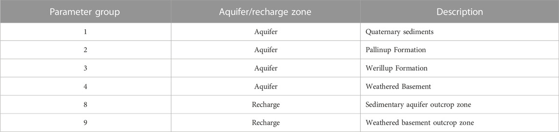
TABLE 2. Parameter group descriptors used in parameter name definitions.

2.2 History matching data, derived metrics, and predictions of interest

The DA, UQ and SA techniques employed in this study were based on historical lake and groundwater levels. These levels have been measured in Lake Muir and groundwater monitoring boreholes drilled as part of hydrogeological investigations by the former Western Australia Department of Land Management (New et al., 2004), and further expanded by former Department of Environment and Conservation (Grelet and Smith, 2009). These groundwater monitoring boreholes have been screened to target the different hydrogeological units in the area and are displayed in Figure 6, along with selected locations from which model results are presented and discussed.

FIGURE 6

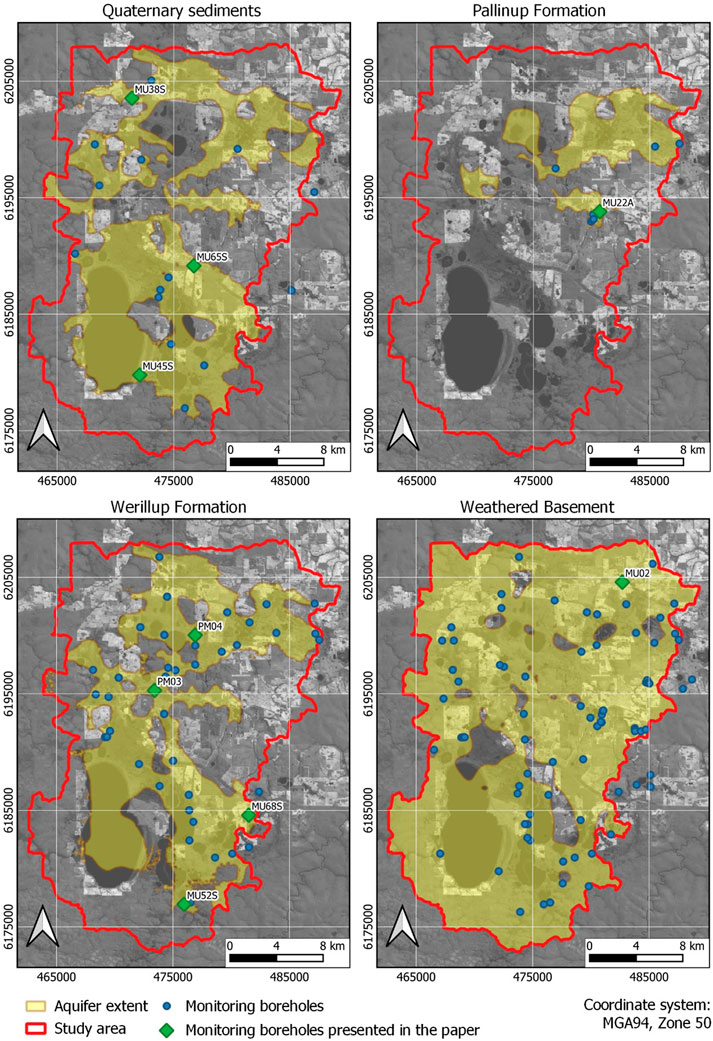
FIGURE 6. Location of groundwater monitoring boreholes screened in the different hydrogeological units.

The majority of the data have been collected on a monthly basis from early 2000s, while historical level measurements on Lake Muir have been conducted since 1980s, mostly during the wet seasons. In the context of impacts related to rainfall decline, the dataset coverage is relatively small, since the decline period started in the early 1970s.

The MUNDRC model used several direct and derived history-matching and predictive metrics, as summarized in Table 3. Direct metrics are defined here as values related to direct model outputs that do not require further post-processing (or in other words, raw output), while derived metrics are based on post-processing of model outputs (such as head-differences). The use of different metrics was three-fold: attempt to improve history matching, reduce parameter and predictive uncertainty, and to understand how they respond to parameter changes and contribute to the reduction of uncertainty.

TABLE 3

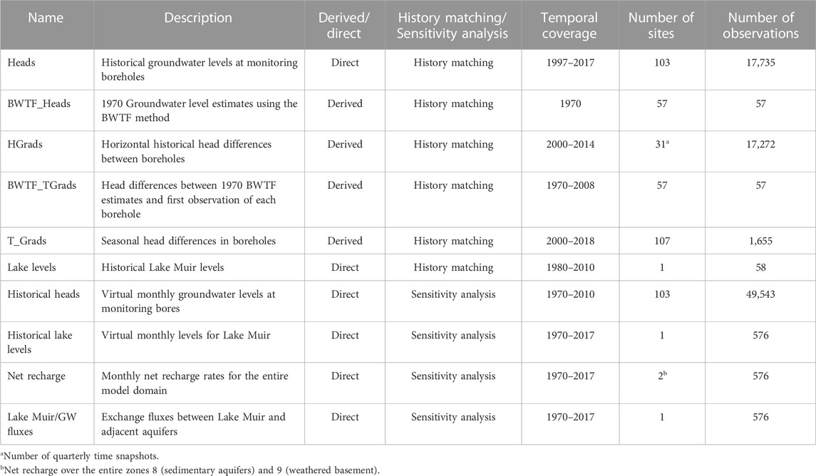
TABLE 3. System observation metrics used in history matching, and predictive metrics used in the UQ and SA workflows.

Horizontal head differences between boreholes were added as observations, based on a Delaunay triangulation generated from the borehole locations. Head differences between borehole pairs defining each of the triangulation edges were use as observations, with quarterly snapshots generated for the period from 2000–2014. Seasonal head differences within each borehole were also included, in an attempt to inform the optimization process of groundwater level differences between wet and dry seasons. Groundwater level estimates for 1970 presented in De Sousa (2021) were included, together with the difference between these levels and the first record of each borehole, in an attempt to inform long-term changes.

In addition, predictive metrics have been added in for the sensitivity analysis workflows in the form of “virtual observations” (i.e., fake observations at prescribed locations in space-time), for sensitivity analysis. Virtual monthly groundwater level observations have been added for all boreholes, covering the period from 1970 to 2010 to observe whether sensitivity to groundwater levels vary over time. Virtual observations for lake levels were also included, in addition to monthly net recharge rates and exchange fluxes between Lake Muir and adjacent aquifers.

3 Data assimilation in conceptualization

3.1 Identifying rainfall decline trends in groundwater monitoring data

Given the strong correlation between rainfall rates and groundwater levels, it was expected that drawdown trends associated to rainfall decline would be strongly present in the historical data, however, the identification of long-term drawdowns in the available monitoring data is very subtle and difficult to undertake. Reasons for that include the relatively short monitoring period (15-year against 40–50 years of rainfall decline) and also that the consistent rainfall decline for such a long period may lead the catchment towards a new equilibrium state, with groundwater levels “adapting” to the lower recharge regime. Lastly, the high seasonality observed in groundwater levels add short-term variations in monitoring records masking subtler long-term drawdown trends.

Here, the EMD method have been applied to the groundwater time series from monitoring boreholes to isolate long-term drawdown terms from seasonal and higher frequency changes in groundwater levels.

Groundwater time series from all monitoring boreholes were processed using the Python implementation of the EMD algorithm developed by Laszuk (2017). The original data and resulting IMF’s for monitoring boreholes MU22A, MU45S and MU65S are presented in Figure 7. The EMD results show long-term decline terms in the last IMF of all three boreholes (IMF_6 for MU22A, IMF_5 for boreholes MU45S and MU65S), while seasonal signals for the three boreholes are clearly identified in IMF’s 3, 1 and 2, respectively.

FIGURE 7

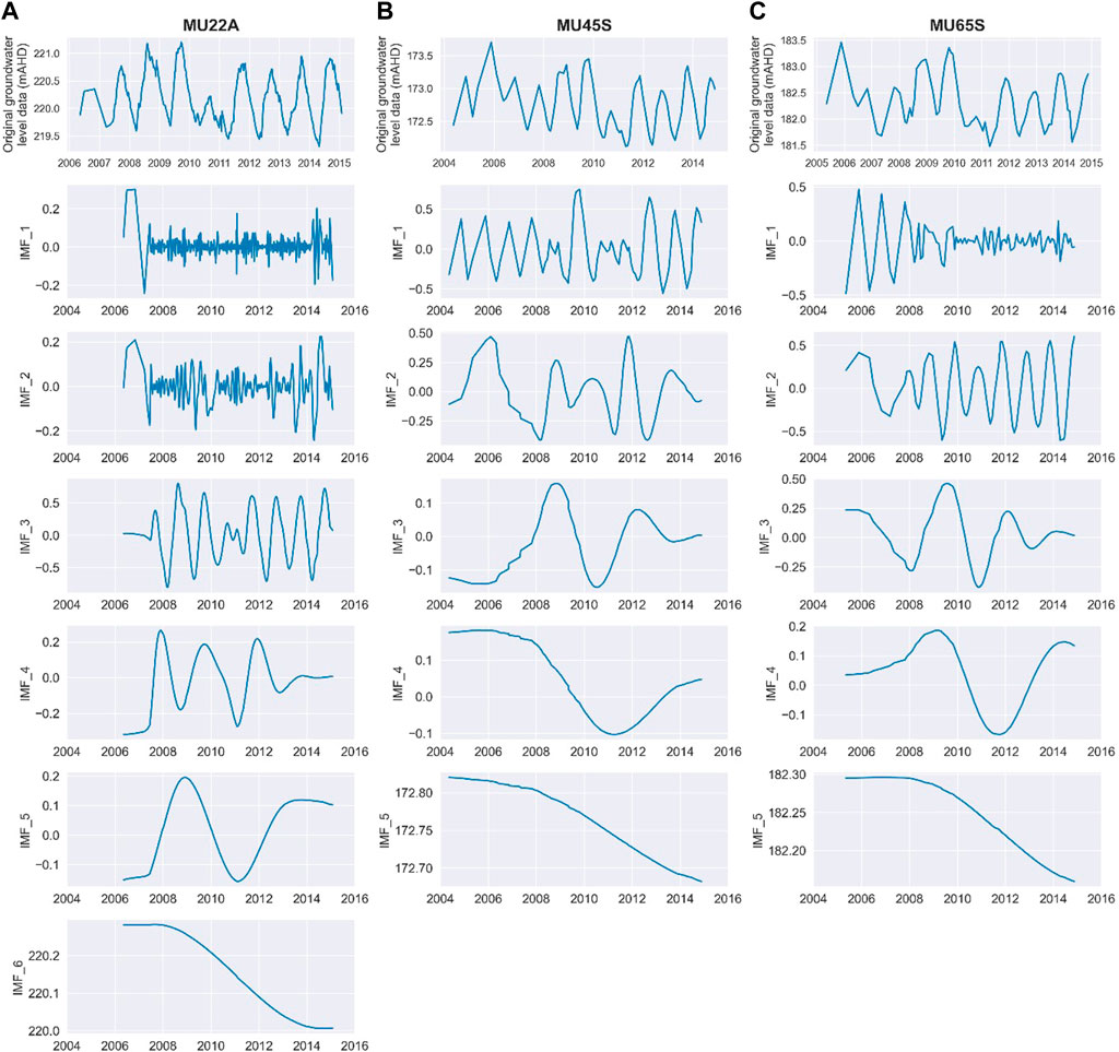
FIGURE 7. Historical groundwater levels and Intrinsic Mode Functions obtained from the EMD analysis for boreholes MU22A (A), MU45S (B) and MU65S (C).

Another important aspect is that the magnitude of the long-term variations found by the EMD are much smaller than seasonal variations in the groundwater levels and higher-frequency IMF’s, demonstrating the ability of the method to identify subtle drawdown patterns in areas under high seasonality effects.

3.2 Establishment of baseline groundwater levels and conceptual drawdown estimates

The assessment of environmental impacts often involves the comparison of current and/or past hydrologic states against states prior to the impact development. The absence of baseline data in these situations makes the assessment of these impacts extremely challenging, both on conceptual and quantitative levels.

In the MUNDRC, while groundwater monitoring data was available for a large number of boreholes spread across the catchment, the majority of groundwater level data was collected from the early 2000s approximately 30 years from the beginning of the rainfall decline. From that perspective, besides subtle drawdown trends observed in the EMD analyses, the premise that rainfall decline promoted groundwater drawdown in the catchment was merely conceptual.

Based on relationships between rainfall and groundwater responses, the Backwards Water Table Fluctuation (BWTF) method was developed. This technique enabled the reconstruction of groundwater levels in the MUNDRC prior to rainfall decline by running the calculations backwards in time and providing reverse hindcasts. Historical groundwater levels were estimated for each borehole in the catchment, utilizing a starting head (equating to the latest observation of each monitoring time series), rainfall fraction applied to rainfall historical time series, specific yield, and a constant outflow term. These parameters were calibrated against available data and ran backwards until 1970, prior to rainfall decline.

The pre-rainfall decline hindcasts obtained from this method provided not only preliminary drawdown estimates across the catchment, but also estimates on net recharge rates. Furthermore, the estimated groundwater levels were incorporated in the forward numerical framework (as discussed in history matching metrics), therefore enabling the history matching to reach for reasonable groundwater levels pre-rainfall decline and provide more robust estimates for groundwater level changes since 1970.

4 Uncertainty quantification and the role of history matching

4.1 Reducing uncertainty

The Iterative Ensemble Smoother implementation in PESTPP-IES have been utilized for history-matching aiming at 1)—reasonably representing historical behavior of the catchment, 2)—reduce parameter uncertainty, 3)—provide an ensemble of conceptually feasible parameter sets that are a reasonable approximation of posterior parameter distributions and 4)—enable the quantification of uncertainty of the different metrics and predictions of interest.

PESTPP-IES was used in conjunction with the numerical model described in the previous section and upgraded here with pilot-point parameterization. An ensemble of 150 realizations was constructed based on conceptual information of the site, which included likely parameter values, upper and lower bounds, and conceptual estimates of spatial correlation. The prior ensemble included a base realization, which served as a parameter means for the remaining realizations. This realization was based on the piecewise-zone calibration presented in De Sousa (2021).

Prior information was applied in the generation of the parameter sets through the definition of parameter means and boundaries as well as their spatial correlations. Upper and lower boundaries for aquifer parameter values were based on lithological descriptions and literature values (Reynolds and Marimuthu, 2007) of each of the aquifers. Parameter bounds for recharge outflow terms were set .7 to 1.2 while values between .5–.9 were assigned to rainfall fraction. The spatial correlation of parameters of the same type and group was defined using covariance matrices based on variograms defined for the area, under the assumption that spatial correlation is lost beyond the distance of 6 km.

Details from the PESTPP-IES settings used in this calibration, including regularization settings and use of localization, are discussed in De Sousa (2021). The results from the history matching showed a reduction in the mean objective function value from 484,555 to 28,936 at the end of iteration 6. The standard deviation of the objective function values also reduces throughout the iterations, from a prior value of 583,308 to 641 at the end of optimization. Furthermore, the total number of runs required for the entire procedure (prior plus 6 iterations) was 1842, which is about half the number of adjustable parameters and demonstrates the efficiency of the algorithm. Despite similar objective functions obtained at the end of the IES optimization, the distribution of parameters from the different ensemble sets can be quite distinct, as illustrated by horizontal conductivity values in layer one displayed in Figure 8. Although the differences between realizations in this figure are not always apparent (since the color-scale span 4 orders of magnitude), the histograms for hydraulic conductivity displayed in Figure 10 show clearly that ranges often span over one order of magnitude.

FIGURE 8

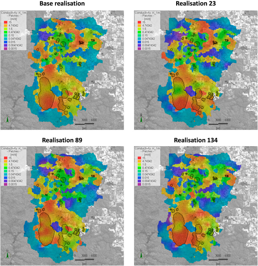
FIGURE 8. Calibrated horizontal conductivity values for layer 1 on selected posterior ensemble realizations.

To illustrate the reduction in uncertainty, simulated hydrographs from the prior and posterior ensemble were plotted against observed data and the results from the piecewise-constant zone calibration presented in De Sousa (2021) for selected monitoring locations and Lake Muir (Figure 9). When compared to the prior ensemble, the posterior realizations not only present a better fit with observed data, but also have a much narrower spread (therefore demonstrating the reduction of parameter uncertainty). In relation to the piecewise-constant calibration, posterior runs also present a significantly better fit, which is expected as the highly-parameterized form allows for heterogeneity within the parameter zones and adjust locally to each monitoring location. Lastly it can be observed that prior realizations are predominantly centered around the hydrographs from the piecewise-constant calibration run, which is expected as the parameters from this run were used as means for the generation of the prior ensemble set.

FIGURE 9

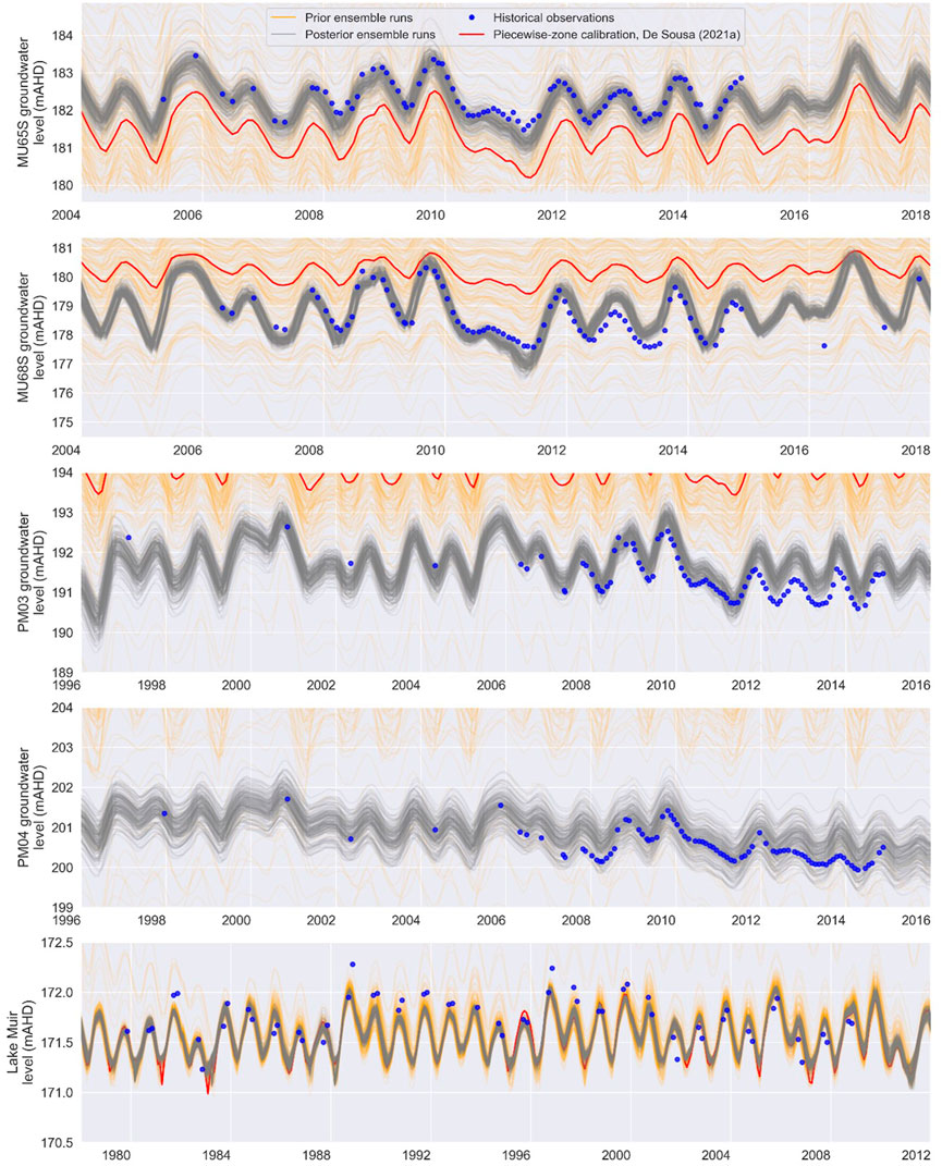
FIGURE 9. Simulated lake and groundwater levels prior and post-calibration at selected locations.

The reduction of uncertainty can also be observed when comparing parameter distributions from prior and posterior ensembles (Figure 10). In this figure, most sensitive parameters to groundwater level observations from selected hydrographs have been selected for plotting of histograms with prior and posterior distributions. It can be observed that there is an overall reduction in the spread of parameter values, and these reductions are particularly pronounced in highly sensitive parameters, such as those related to groundwater recharge. Parameters with low sensitivity such as vertical anisotropy shows little to no reduction in parameter uncertainty.

FIGURE 10

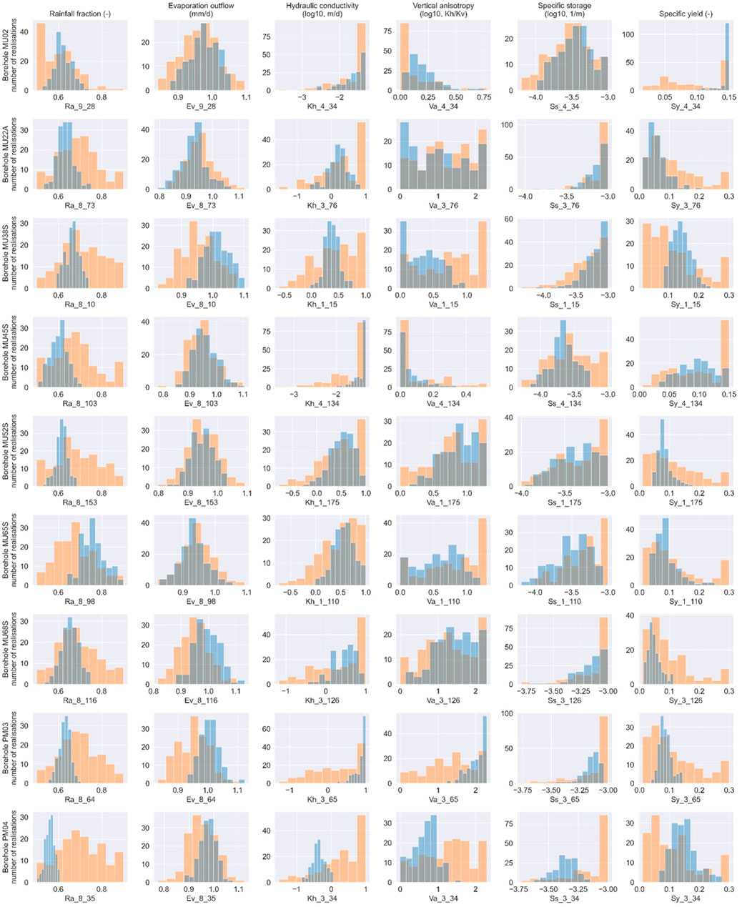
FIGURE 10. Parameter histograms of prior (orange) and posterior (blue) distributions of most sensitive parameters to observations in selected monitoring boreholes.

4.2 Quantification of predictive uncertainty

If the ensemble size utilized by the iterative ensemble smoother is of sufficient size, the execution of model runs using the posterior ensemble sets can be utilized collectively to define posterior probability distributions for predictions of interest.

The results from the posterior ensemble sets obtained using PESTPP-IES were used to assess uncertainty of predicted groundwater levels and other metrics as illustrated in Figures 11 and 12.

FIGURE 11

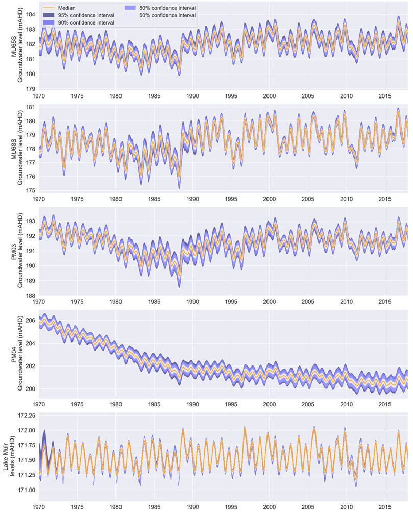
FIGURE 11. Simulated lake and groundwater level ensemble percentiles at selected locations.

FIGURE 12

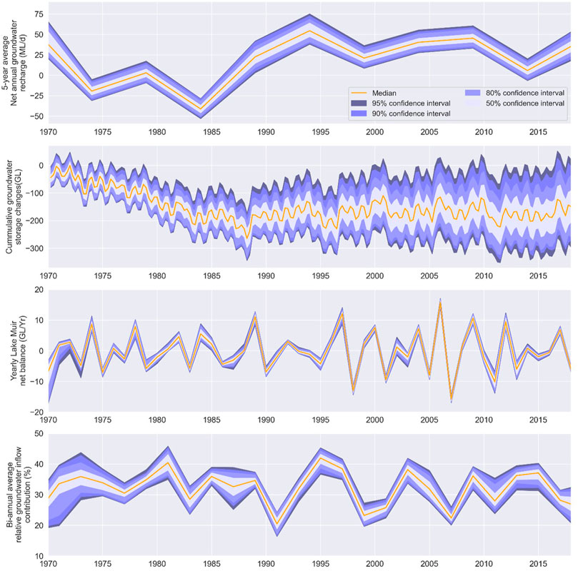
FIGURE 12. Simulated ensemble percentiles for different water balance predictive metrics.

Despite the large number of locations and metrics, some common uncertainty patterns can be observed across different model results. For instance, uncertainty of simulated groundwater levels shows an increase during the period from 1980 to 1988 in many borehole locations such as MU68S and PM03. For these boreholes the maximum simulated drawdown occurs in this period, which suggest the degree of uncertainty is related to the magnitude of stresses being imposed in the catchment. The distribution of mean and standard deviation of simulated groundwater levels corroborates this hypothesis, with areas of larger standard deviation predominantly overlapping areas of larger mean drawdown.

The uncertainty around groundwater levels is relatively small when considering the absolute groundwater levels, with 95% confidence intervals under ±1 m from mean levels for the majority of monitoring boreholes. Nevertheless, when looked in terms of drawdown, these uncertainties can equate to 50%–100% of maximum simulated drawdown in some boreholes (PM-03, MU65S).

Uncertainty around the Lake Muir levels is relatively small, probably due to the fact the dominant fluxes in the lake are controlled by historical rainfall and evaporation time series (prescribed in the model) and only two parameters with corresponding multipliers, as relative contributions from groundwater into the lake inputs only account for approximately 30% (Figure 12).

Uncertainty of mass balance quantities displayed in the same figure provide some important insights. It can be noted that uncertainty over cumulative groundwater storage changes increase progressively through the entire simulated period, where uncertainty around rates such as net recharge and groundwater contributions to lake inflow remain relatively stable. Uncertainties around the period of 1970–1974 are slightly higher for net groundwater recharge, net balance for Lake Muir and relative contributions, as well as lake levels. This is the period where rainfall decline starts and it is possible that the sudden shift in rainfall rates produced larger stresses in the initial years and, consequently larger uncertainty.

5 Sensitivity analysis

We explored different sensitivity analysis techniques and their ability to contribute to the understanding of hydrologic processes occurring in the MUNDRC and terminal catchments in general. Local sensitivity analysis was employed to quantify point-source sensitivities (i.e., at a single location in parameter space) to understand spatial and temporal relationships, and global sensitivity methods were used to provide more robust sensitivity estimates and investigate broader controls on history matching and predictions of interest.

5.1 Improving understanding and conceptualization

A Jacobian matrix for the MUNDRC model has been generated for the parameter set with lowest residuals from the posterior ensemble obtained for the PESTPP-IES history matching work, using PEST-HP. The matrix was constructed considering all parameters (3,295) using a 3-point derivative approximation, in a total of 6,591 model runs. Analyzed inputs included observation and derived metrics used in the history-matching process, as well as virtual observations described in Section 2.2.

The comparison of groundwater level sensitivities to model parameters against the distance between monitoring point and pilot-point location is useful to establish distance-sensitivity relationships and estimate the “radius of influence” of certain parameters. Figure 13 shows plots of absolute sensitivity of groundwater levels in selected monitoring locations, where average sensitivity values for all groundwater levels in each location were calculated for all spatially distributed parameters (i.e., parameters from the pilot points). These plots show that in general, all parameters beyond 2–4 km from observation points show very low to no sensitivity, despite the maximum sensitivity of each parameter group (for example, recharge parameters show very high sensitivity for pilot points within 2–4 km, but the sensitivity is lost in parameters beyond that distance in the same way that storage parameters, which have much lower sensitivities).

FIGURE 13

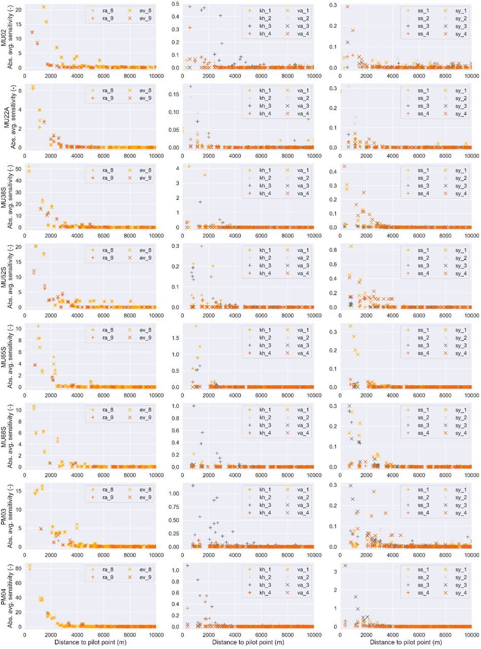
FIGURE 13. Scatter plots of absolute sensitivity values versus distance to pilot point for selected monitoring locations.

The distance-sensitivity plots also unravel relationships between maximum sensitivity on a parameter group basis, and their sensitivity noise, defined here as average groundwater level sensitivities to parameters located beyond the threshold distance. Ratios between maximum sensitivity and sensitivity noise are very high in parameter groups with high maximum sensitivity (such as Ev and Ra), but this ratio tends to degrade for parameter groups with low maximum sensitivity (for example, for groups Ss_3 and Sy_3 in monitoring borehole PM-03).

The use of virtual observations over the entire period between 1970 and 2010 showed that groundwater level sensitivity varies considerably over the simulated period. The assessment of sensitivities over time shows that sensitivity to recharge parameters increase over time (particularly in monitoring bores located away from lakes and other surface water compartments), suggesting that changes in net recharge rates have a cumulative effect on groundwater levels. In monitoring sites near lakes, this cumulative behavior is likely dampened by the model boundary conditions, as groundwater fluxes into these compartments adjust to the different recharge rates.

It can be observed that the sensitivities have a large influence from the rainfall signal, as sensitivity peaks from different parameters and location often align in periods of high or very low rainfall (such as years 2001 and 2006). This also demonstrates that sensitivity is influenced by the magnitude of hydrologic stress throughout the simulated period. Lastly the temporal behavior of storage parameter sensitivities is largely cyclical over the entire simulated period. To investigate whether these oscillations were associated with the seasonality observed in the catchment, groundwater level sensitivities to the parameters were grouped monthly and displayed as box and whiskers plots in Figure 14. These plots show that the groundwater level sensitivity is not only seasonal for storage parameters but, to a lesser degree, all other parameter types. High sensitivity peaks in these plots are normally in April-May, at the end of dry season, and low peaks are observed in September-October, at the end of wet season. This reflects not only the seasonality, but also suggest that the sensitivity is dependent on the hydrological state of the system, with sensitivities varying largely from periods of water surplus (wet season) and water deficit (dry season).

FIGURE 14

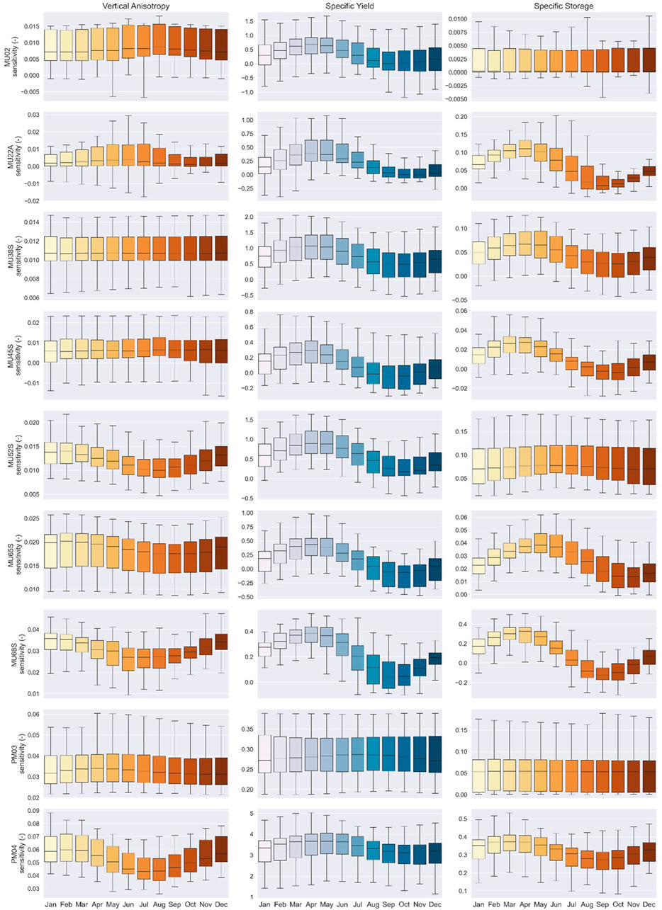
FIGURE 14. Monthly-grouped absolute sensitivity values for vertical anisotropy, specific yield and specific storage at selected locations.

5.2 Assessing the value of history matching metrics and prioritizing site investigation efforts with linear uncertainty methods

Doherty and Hunt (2009) describe two statistics referred to as Identifiability and Relative Parameter Uncertainty Variance Reduction (RUVR). These statistics can be obtained from the Jacobian Matrix of a calibrated parameter set for any adjustable parameter and vary between 0 and 1, where the value of 0 means no reduction of uncertainty has been achieved through the history-matching process and the value of 1 indicates small parameter uncertainty in relation to the prior.

These analyses can be obtained considering history-matching observations that exist or not, and when applying different settings for observations (through weighting) and parameters (by fixing them or not) they can provide useful insights on the value of different observation groups, aggregate value of raw and derived metrics, and also inform site investigation efforts.

The several history-matching groups employed in the calibration of the MUNDRC model allowed a significant reduction in parameter uncertainties and also reasonable replication of past system behavior. However, the contribution of the different metrics to reduction in the uncertainty of different parameter groups was not clear. To investigate that, different linear analysis runs were done considering the entire history-matching data set and different observation groups individually as displayed in Figure 15, where values for identifiability and RUVR were averaged for the different parameter groups.

FIGURE 15

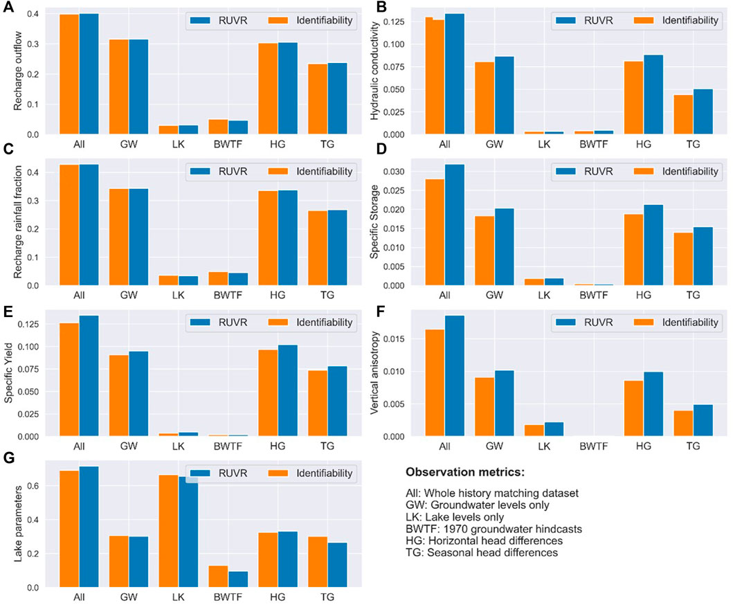
FIGURE 15. Average identifiability and RUVR values considering the entire history matching data set and individual metrics for (A) Recharge outflow term, (B) Horizontal hydraulic conductivity, (C) Recharge rainfall fraction, (D) Specific storage, (E) Specific yield, (F) Vertical anisotropy, and (G) Lake parameters.

These results shows that 1) the sum of the values from individual observation groups is different from the values for the entire dataset, given the fact the these metrics are to some extent correlated in terms of sensitivity, 2) groundwater level observations shown overall the largest identifiability values as an individual group, 3) contributions from the derived metrics of horizontal and seasonal head differences to reduction of parameter uncertainty are most effective in the identification of storage parameters and 4) identifiability and RUVR values for lake values are predominantly controlled by lake observations, with subordinate contributions of groundwater levels. In the case of horizontal head differences, it also shows slightly higher values than the raw groundwater levels, showing that they have the same ability, if not more, of reducing parameter uncertainty.

In order to inform further investigation efforts in the area, additional linear analysis runs were undertaken by fixing the different parameter groups to understand what the reductions in the uncertainty of the remaining parameters would be if the fixed parameters were known. These results show clearly that largest benefits in terms of reducing parameter uncertainty would be from investigating recharge attributes (either infiltration rates, Ra, or evapotranspiration, Ev) as they would result in a minimum of 10% increase in identifiability values (with exception of lake parameters). The determination of unconfined storage (i.e., specific yield) would also be beneficial, as it controls the effective size of groundwater reservoir and the magnitude of head change associated with net recharge.

6 Discussion

6.1 The use of DA, UQ and SA techniques throughout the model development

While the DA, UQ and SA techniques are mostly used as accessories in conventional modelling practice, they have proven pivotal to the development of the numerical model and evolution of conceptual understanding of the MUNDRC. Where in earlier stages of model development the definition of aquifer geometry, boundary conditions and coupling with the lake model were reasonably straightforward, the initial iterations of history matching and conceptualization were hindered by the lack of baseline groundwater level data. At that stage, despite the clear reduction of rainfall volumes, groundwater and lake level declines could not be clearly demonstrated.

The application of EMD on historical groundwater levels provided some evidence of longer-term drawdowns, by removing noise introduced by seasonal and higher-frequency variations, supporting the hypothesis that groundwater levels dropped as result of rainfall decline. While not employed in this study, the EMD’s ability to decompose time series in different frequencies could enable new derived metrics for history matching by comparing simulated and observed IMF’s, similar to the “data transformation methods” described in Bennett et al. (2013) and the “Metrics describing multi-scale variability in model state” from Hipsey et al. (2020). These metrics potentially can contribute to history matching and robustness of models by highlighting aspects of model behavior that are not clear in the original time domain.

The high correlation between seasonality of groundwater levels and rainfall led to attempts of establishing relationships between rainfall rates, net groundwater recharge and groundwater levels. These attempts culminated in the development of the BWTF, which provided coarse estimates on net recharge but, most importantly, provided hindcast estimates of groundwater levels in 1970, prior to rainfall decline. The baseline groundwater level estimates from the BWTF analysis allowed for: 1—Reconstruction of groundwater levels prior to the rainfall decline (from a conceptual perspective), 2—Inclusion of these estimates in the history matching process, 3—Improvement of recharge implementation in the groundwater model by using a similar formulation and 4—Simulation of the whole trajectory from pre-rainfall decline towards present day.

Once the final model form was in place (1960–2018 simulated period with BWTF estimates in history matching, coupled lake model and improved recharge formulation), the history matching techniques assisted in reducing the uncertainty around aquifer parameters, which was particularly important since no aquifer test data was available. The piecewise-zone calibration presented in De Sousa (2021) provided reasonable average values for the entire catchment, and the highly-parameterized form presented in this paper allowed better representation of historical system behavior, representation of heterogeneity within each of the hydrogeological units and implemented the foundation for the UQ workflows.

The IES technique employed in history matching provided a quantitative assessment of parameter and predictive uncertainty constrained solely by conceptual expert-knowledge (i.e., prior) and allowed data assimilation in its more classic form, where prior model uncertainty has been reduced through the assimilation of site observations (i.e., history matching).

This paper has presented the final results of sensitivity analysis; nevertheless, several iterations have been undertaken throughout the development of the model, many of which contributed to the final form of conceptual and numerical model. The investigation of distance-sensitivity relationships provided insights on the area of influence of each parameter and this information can be helpful in the use of localization in iterative ensemble smoothers (Chen and Oliver, 2013). These relationships can also be used to prioritise site investigations, particularly if used in conjunction with linear uncertainty analysis.

Transient and seasonal trends of groundwater level sensitivity identified in the model demonstrate the value of using virtual observations over the entire simulated periods, even when corresponding field measurements are not available. Although these sensitivities cannot be used in the history matching process, they were useful to establish relationships between seasonality, aquifer net balance state (surplus, deficit or neutral) and sensitivity.

6.2 Distinct attributes of terminal catchments unveiled by these techniques

The results from the DA, UQ and SA techniques corroborated several attributes of the MUNDRC that are distinct of low-relief terminal catchments and unveiled new attributes that were expected by early conceptualization.

The sensitivity analysis of the Jacobian matrix showed the dominance of recharge parameters in terms of sensitivity and confirm the high influence of the interplay between rainfall infiltration and evapotranspiration in groundwater levels and catchment dynamics. Regarding groundwater levels, the conceptualization postulated that their response to rainfall events was rapid given the shallow groundwater table depths and relatively high hydraulic conductivity of sedimentary aquifers. The results from the BWTF and FEFLOW models agree with this hypothesis, as a good fit between simulated and groundwater levels was obtained for absolute values and seasonal oscillations without the use of a delay term in the recharge formulations. Furthermore, cluster analysis also demonstrated the relationships between land use and groundwater recharge, as well as its influence in associated groundwater level signatures.

The analysis of model results also led to some insights that were counter-intuitive and in disagreement with our early conceptualization. For instance, groundwater inflows into Lake Muir were expected to be higher during the dry season as the lake levels were at their lowest. Mass balance analysis of FEFLOW showed that while that is true in terms of relative contributions, the highest groundwater discharge rates occur during the wet season, where highest recharge rates replenish the aquifers increasing hydraulic gradients and consequently discharge rates. In another example, it was expected that groundwater discharge would occur predominantly through the base of the lake (assuming density effects on groundwater head distribution were negligible). Mass balance results at the lake nodes suggest that fluxes from lake to the aquifers occur through the base of the lake, groundwater discharge into Lake Muir occurs predominantly along the perimeter of the lake (De Sousa, 2021). Lastly, groundwater levels near surface water compartments are less sensitive to recharge and are to some extent regularized, in the sense that changes in recharge rates and groundwater level are compensated by adjusted flux rates between surface water bodies and adjacent aquifers.

Another new concept unveiled by the SA was the transient sensitivity of groundwater levels with regards to time. While this concept seems straight forward after the analysis of results, the concept of transient sensitivities has not, to the authors’ knowledge, been demonstrated in literature.

The discussion presented in De Sousa (2021) suggests that Lake Muir is more resilient to rainfall decline the originally thought. The UQ works presented in this paper corroborate that and sensitivity analysis hinted at the underlying reasons. It was observed that sensitivity to rainfall multiplier (Lk_rain) was in general higher than sensitivity to the evaporation multiplier (Lk_evap), leading to the conclusion while evaporation rates are directly related to the lake area, rainfall rates are less susceptible to that as rainwater infiltrates the dry portions of the lake and ultimately is discharged there. The direct relation between lake area and evaporation volumes can be translated to lake level and evaporation volumes, therefore decline in lake levels caused by rainfall decline (both as direct rainfall and groundwater discharge) incur reduced evaporation rates, dampening the net lake losses. This is a mechanism that can be extrapolated to all lakes with shallow and flat bathymetry, but less likely to occur in lakes with steeper lake beds, as reductions in lake area (and evaporation) due to decline in lake level will be somewhat smaller.

6.3 Computational costs and limitations of the different techniques

The results presented in the previous sections demonstrate the value of DA, UQ and SA techniques in improving conceptual understanding and facilitating the quantification of impacts and catchment hydrologic processes. On the other hand, computation costs of each of these techniques may lead to a prioritization of efforts and cost/benefit assessment in a resource-constrained study. Furthermore, the use of these techniques needs to be undertaken cognizant of their limitations and computational costs, some of which are discussed here.

The use of the EMD method is computationally inexpensive and can be used in a batch fashion to process time series from multiple observation time series simultaneously, but the interpretation of the Intrinsic Mode Functions obtained from the EMD must be conducted with caution as they can be highly sensitive to the time series sampling frequency and are potentially problematic when time series have irregular observation intervals. This can be noticed on the analysis for borehole MU22A (Figure 7) which has a higher monitoring frequency and display an additional high frequency IMF when compared to the time series from boreholes MU45S and MU65S. It is possible that this issue could be minimized by resampling at regular intervals using interpolation methods and, despite not being tested, the application of EMD on the regular time series generated by the BWTF method may prove to be a better option than the raw monitoring data.

The IES method is an extremely powerful approach that allows history matching of highly-parameterized models with a very small number of runs, compared to number of parameters, enabling DA and UQ of large models that would previously be too expensive in terms of computational effort. While the IES method has shown good history matching results with small ensemble sizes (in particularly if localization is employed), questions remains whether these ensembles are sufficiently large to characterize the uncertainty, particularly in terms of probability distributions. A possible solution for that could potentially be to increase the ensemble size with parameter sets derived from the sampling of a posterior covariance matrix created based on the original ensemble parameter values. This procedure would continue to require a small number of runs for the history matching process and provide a larger ensemble size for UQ. Furthermore, the application of ensemble methods in groundwater modelling is relatively new and more testing and use of this tool is required for definition of optimized settings such as ensemble size, localization matrices and so forth.

The DA and UQ applied in the MUNDRC model resulted in simulated groundwater and lake levels with relatively small uncertainty. It is important to emphasize, however, that the rainfall time series for the simulated period were actual values from historical records and “hard-wired” in the model lake and recharge components. Given that there is a strong relationship between groundwater level, sensitivity, and rainfall rates/events (as seen in the transient sensitivity plots), groundwater predictions in the future should account for uncertainty of rainfall time series inputs, and these can potentially promote larger predictive uncertainty.

7 Conclusion

The research presented in this paper illustrates the use of DA, UQ and SA in the study of terminal catchments, their value in the identification of particularities of hydrologic behavior in these settings and provide a blueprint for assessment of impacts associated to long-term rainfall decline in terminal catchments. On a conceptual level, main drivers of the groundwater and surface-groundwater interactions have been identified and corroborated by sensitivity analysis results. In terms of quantification and prediction, the developed numerical model coupling approaches and data assimilation tools used in the study provide a framework to estimate environmental impacts considering inherent hydrogeological and hydrological uncertainty, as well as the ability of monitoring data to constrain it. From a broader perspective, practicalities and lessons learned from the application of these techniques are lacking in literature, which is predominantly focused on theory and development of new techniques, and the paper also contributes to that regard.

Although several techniques have been explored in this study, it by no means exhaust the number of techniques available in the literature. Notable examples include the time-series analysis using transfer function noise modelling (Collenteur et al., 2019), evolutionary algorithms (Maier et al., 2014), time series clustering methods (Aghabozorgi et al., 2015) and ensemble machine learning techniques (Zounermat-Kermani et al., 2021).

This study has also shown that much can be gained through feedback loops between the application of these techniques (in particular SA) and conceptualization, as opposed to conventional use of UQ and SA at the end of model development. The conceptual model of MUNDRC have evolved substantially from its early inception through the multiple sensitivity analysis rounds until the final conceptual and numerical model form was achieved. Counter-intuitive findings from this process such as higher groundwater inflows to Lake Muir during the wet season, dominance of vertical dynamics of recharge and evapotranspiration over horizontal flows and potential surface runoff flows into the lake challenged the assumptions from initial conceptualization and resulted in a more robust final model form which conforms to expert-knowledge and was able to replicate historical system behavior.

The DA, UQ and SA techniques applied in the MUNDRC were undertaken with open-source software freely available on web which facilitated the model development significantly. Nevertheless, the implementation these techniques still remains an onerous task, particularly with regards to post-processing workflows. The adoption of these techniques in the broader modelling community will depend much on the development of tools to streamline these workflows and availability of educational resources, and initiatives such as the Groundwater Modelling Decision Support Initiative (GMDSI, https://gmdsi.org) are making a big impact in that direction.

Data availability statement

The original contributions presented in the study are included in the article/supplementary materials, further inquiries can be directed to the corresponding author.

Author contributions

The numerical framework and application of the different DA, UQ, and SA techniques to the models, as well as findings from the interpretation of model results and writing of the manuscript have been developed by ED, under supervision of the co-authors, who also provided feedback during the uncertainty and sensitivity analyses, contributed to the final format of the paper, editing and review of the manuscript, and also checked the scientific integrity of the research.

Funding

This research was supported by an Australian Government Research Training Program (RTP) Scholarship.

Acknowledgments

The authors would like to acknowledge Jasmine Rutherford, Roger Hearn, and Margaret Smith (former Western Australia Department of Environment and Conservation) for providing the geology and groundwater monitoring data, as well as technical support and discussions about the MUNDRC hydrogeology.

Conflict of interest

Author ED was employed by the company INTERA Inc. Author RV was employed by the company Hydrogeoenviro Pty Ltd.

The remaining author declares that the research was conducted in the absence of any commercial or financial relationships that could be construed as a potential conflict of interest.

Publisher’s note

All claims expressed in this article are solely those of the authors and do not necessarily represent those of their affiliated organizations, or those of the publisher, the editors and the reviewers. Any product that may be evaluated in this article, or claim that may be made by its manufacturer, is not guaranteed or endorsed by the publisher.

References

Aghabozorgi, S., Shirkhorshidi, A. S., and Wah, T. Y. (2015). Time-series clustering – a decade review. Inf. Syst. 25, 16–38. doi:10.1016/j.is.2015.04.007

CrossRef Full Text | Google Scholar

Asch, M., Bocquet, M., and Nodet, M. (2016). Data assimilation: Methods, algorithms and applications. Philadelphia, Pensylvania: Society for Industrial and Applied Mathematics, 311.

Google Scholar

Bennett, N. D., Croke, B. F. W., Guariso, G., Guillaume, J. H. A., Hamilton, S. H., Jakeman, A. J., et al. (2013). Characterising performance of environmental models. Environ. Model. Softw. 40, 1–20. doi:10.1016/j.envsoft.2012.09.011

CrossRef Full Text | Google Scholar

Chen, Y., and Oliver, D. S. (2013). Levenberg–Marquardt forms of the iterative ensemble smoother for efficient history matching and uncertainty quantification. Comput. Geosci. 17 (4), 689–703. doi:10.1007/s10596-013-9351-5

CrossRef Full Text | Google Scholar

Collenteur, R. A., Bakker, M., Calje, R., Klop, S. A., and Schaars, F. (2019). Pastas: Open-Source software for the analysis of groundwater time series. Groundwater 57 (6), 877–885. doi:10.1111/gwat.12925

PubMed Abstract | CrossRef Full Text | Google Scholar

Dausman, A. M., Doherty, J., Langevin, C. D., and Sukop, M. C. (2010). Quantifying data worth toward reducing predictive uncertainty. Ground Water 48 (5), 729–740. doi:10.1111/j.1745-6584.2010.00679.x

PubMed Abstract | CrossRef Full Text | Google Scholar

De Sousa, E. R. (2021). Evaluation of long-term rainfall decline impacts on small-scale semi-arid endorheic basins and application to Lake Muir-Unicup Natural Diversity Recovery Catchment. PhD Thesis. Perth, Australia: School of Agriculture and Environment, University of Western Australia.

Google Scholar

Diersch, H.-J. G. (2014). FEFLOW finite element modeling of flow, mass and heat transport in porous and fractured media. Berlin, Germany: Springer-Verlag, 996.

Google Scholar

Doherty, J. (2015). Calibration and Uncertainty Analysis for complex environmental models. Brisbane: Watermark Numerical Computing, 236.

Google Scholar

Doherty, J., Fienen, M., and Hunt, R. (2010). Approaches to highly parameterized inversion: Pilot point theory, guidelines, and research directions. Reston, Virginia: USGS Scientific Investigations. Technical report: Report 2010-5168.

Google Scholar

Doherty, J., and Hunt, R. J. (2009). Two statistics for evaluating parameter identifiability and error reduction. J. Hydrology 366, 119–127. doi:10.1016/j.jhydrol.2008.12.018

CrossRef Full Text | Google Scholar

Doherty, J. (2020). PEST_HP - PEST for highly parallelized computing environments. Brisbane, Australia: Watermark Numerical Computing.

Google Scholar

Ferdowsian, R., Pannel, D. J., McCarron, C., Ryder, A., and Crossing, L. (2001). Explaining groundwater hydrographs: Separating atypical rainfall events from time trends. Aust. J. Soil Res. 39, 861. doi:10.1071/sr00037

CrossRef Full Text | Google Scholar

Gallagher, M., and Doherty, J. (2020). Water supply security for the township of biggenden: A GMDSI worked example report. South Australia: National Centre for Groundwater Research and Training, Flinders University.

Google Scholar

Gong, Y., Wang, Z., Xu, G., and Zhang, Z. (2018). A comparative study of groundwater level forecasting using data-driven models based on ensemble empirical mode decomposition. Water 10, 730. doi:10.3390/w10060730

CrossRef Full Text | Google Scholar

Grelet, G., and Smith, M. G. (2009). The Lake muir–unicup natural diversity Recovery catchment drilling Program: Completion report 2003–2006. Perth, Western Australia: Department of Environment and Conservation, Bore Completion Report. (unpublished).

Google Scholar

Hill, M. C., and Tiedeman, C. R. (2007). Effective groundwater model calibration. Hoboken NJ: Wiley.

Google Scholar

Hipsey, M. R., Gal, G., Arhonditsis, G. B., Carey, C. C., Elliot, J. A., Frassl, M. A., et al. (2020). A system of metrics for the assessment and improvement of aquatic ecosystem models. Environ. Model. Softw. 128, 104697. doi:10.1016/j.envsoft.2020.104697

CrossRef Full Text | Google Scholar

Hope, P., and Foster, I. (2005). How our rainfall has changed – the south-west. Climate Note 5/05. Perth, Western Australia: Indian Ocean Climate Initiative.

Google Scholar

Huang, N. E., Shen, Z., Long, S. R., Wu, M. C., Shih, H. H., Zheng, Q., et al. (1998). The empirical mode decomposition and the Hilbert spectrum for nonlinear and non-stationary time series analysis. Proc. R.Soc. Lnd. 454, 903–995. doi:10.1098/rspa.1998.0193

CrossRef Full Text | Google Scholar

James, S. C., Doherty, J. E., and Eddebbarh, A. (2009). Practical post-calibration uncertainty analysis: Yucca Mountain, Nevada. Ground Water 47 (6), 851–869. doi:10.1111/j.1745-6584.2009.00626.x

PubMed Abstract | CrossRef Full Text | Google Scholar

Jolly, I. D., McEwan, K. L., and Holland, K. L. (2008). A review of groundwater-surface water interactions in arid/semi-arid wetlands and the consequences of salinity for wetland ecology. Ecohydrology 1, 43–58. doi:10.1002/eco.6

CrossRef Full Text | Google Scholar

Lafare, A. E. A., Peach, D. W., and Hughes, A. G. (2016). Use of seasonal trend decomposition to understand groundwater behaviour in the Permo-Triassic Sandstone aquifer, Eden Valley, UK. Hydrogeology J. 24, 141–158. doi:10.1007/s10040-015-1309-3

CrossRef Full Text | Google Scholar

Laszuk, D. (2017). Python implementation of empirical Mode decomposition algorithm. GitHub repository. Available at: https://github.com/laszukdawid/PyEMD. doi:10.5281/zenodo.5459184

CrossRef Full Text | Google Scholar

Maheshwari, S., and Kumar, A. (2014). Empirical mode decomposition: Theory and applications. Int. J. Electron. Electr. Eng. 7 (8), 873–878.

Google Scholar

Maier, H. R., Kapelan, Z., Kasprzyk, J., Kollat, J., Matott, L. S., Cunha, M. C., et al. (2014). Evolutionary algorithms and other metaheuristics in water resources: Current status, research challenges and future directions. Environ. Model. Softw. 62, 271–299. doi:10.1016/j.envsoft.2014.09.013

CrossRef Full Text | Google Scholar

Moore, C., and Doherty, J. (2006). The cost of uniqueness in groundwater model calibration. Adv. Water Resour. 29, 605–623. doi:10.1016/j.advwatres.2005.07.003

CrossRef Full Text | Google Scholar

New, C. E. S., Smith, R. A., Hearn, R. W., and Wheeler, I. B. (2004). “Groundwater-lake interactions in the Lake muir-unicup Recovery catchment [online],” in Engineering Salinity Solutions: 1st National Salinity Engineering Conference 2004. Editors S. Dogramaci, and A. Waterhouse (Barton, A.C.T: Engineers Australia), 460–465.

Google Scholar

Nicols, C., and Doherty, J. (2020). Exploring model defects using linear analysis: A GMDSI worked example report. South Australia: National Centre for Groundwater Research and Training, Flinders University.

Google Scholar

Pianosi, F., Beven, K., Freer, J., Hall, J. W., Rougier, J., Stephenson, D. B., et al. (2016). Sensitivity analysis of environmental models: A systematic review with practical workflow. Environ. Model. Softw. 79, 214–232. doi:10.1016/j.envsoft.2016.02.008

CrossRef Full Text | Google Scholar

Reynolds, D. A., and Marimuthu, S. (2007). Deuterium composition and flow path analysis as additional calibration targets to calibrate groundwater flow simulation in a coastal wetlands system. Hydrogeology J. 15, 515–535. doi:10.1007/s10040-006-0113-5

CrossRef Full Text | Google Scholar

Saltelli, A., Ratto, M., Andres, T., Campolongo, F., Cariboni, J., GatelliSaisana, D. M., et al. (2008). Global sensitivity analysis—the primer. Chichester, West Sussex: John Wiley & Sons, 292.

Google Scholar

Saltelli, A., Tarantola, S., Campolongo, F., and Ratto, M. (2004). Sensitivity analysis in practice—a guide to assessing scientific models. Chichester, West Sussex: John Wiley & Sons, 219.

Google Scholar

Seeboonruang, U. (2014). An empirical decomposition of deep groundwater time series and possible link to climate variability. Glob. NEST J. 16 (1), 87–103.

Google Scholar

Thompson, S. E., Sivapalan, M., Harman, C. J., Srinivasan, V., Hipsey, M. R., Reed, P., et al. (2015). Developing predictive insight into changing water systems: Use-inspired hydrologic science for the anthropocene. Hydrology Earth Syst. Sci. 17 (12), 5013–5039. doi:10.5194/hess-17-5013-2013

CrossRef Full Text | Google Scholar

Wang, Z., Zhao, H., Sheng, Y., Geng, J., Wang, K., and Yang, H. (2020). Groundwater net discharge rates estimated from lake level change in Badain Jaran Desert, Northwest China. Sci. China, Earth Sci. 63 (5), 713–725. doi:10.1007/s11430-019-9533-8

CrossRef Full Text | Google Scholar

Welter, D. E., White, J. T., Hunt, R. J., and Doherty, J. E. (2015). Approaches in highly parameterized inversion— PEST++ Version 3, a Parameter ESTimation and uncertainty analysis software suite optimized for large environmental models. Reston, Virginia: U.S. Geological Surbey, 54. U.S. Geological Survey Techniques and Methods, book 7, chap. C12.

Google Scholar

White, J. T. (2018). A model-independent iterative ensemble smoother for efficient history-matching and uncertainty quantification in very high dimensions. Environ. Model. Softw. 109, 191–201. doi:10.1016/j.envsoft.2018.06.009

CrossRef Full Text | Google Scholar

White, J. T., Doherty, J. E., and Hughes, J. D. (2014). Quantifying the predictive consequences of model error with linear subspace analysis. Water Resour. Res. 50 (2), 1152–1173. doi:10.1002/2013WR014767

CrossRef Full Text | Google Scholar

White, J. T., Fienen, M. N., and Doherty, J. E. (2016). pyEMU: a python framework for environmental model uncertainty analysis, version .01. U.S. Geological Survey software release. doi:10.5066/F75D8Q01

CrossRef Full Text | Google Scholar

Zounermat-Kermani, M., Batelaan, O., Fadaee, M., and Hinkelmann, R. (2021). Ensemble machine learning paradigms in hydrology: A review. J. Hydrology 598, 126266. doi:10.1016/j.jhydrol.2021.126266

CrossRef Full Text | Google Scholar