
95% of researchers rate our articles as excellent or good
Learn more about the work of our research integrity team to safeguard the quality of each article we publish.
Find out more
TECHNOLOGY AND CODE article
Front. Earth Sci. , 30 September 2022
Sec. Hydrosphere
Volume 10 - 2022 | https://doi.org/10.3389/feart.2022.884766
This article is part of the Research Topic Rapid, Reproducible, and Robust Environmental Modeling for Decision Support: Worked Examples and Open-Source Software Tools View all 19 articles
 Edom Moges1*
 Benjamin L. Ruddell2
 Liang Zhang1
 Jessica M. Driscoll3
 Parker Norton3
 Fernando Perez1
 Laurel G. Larsen1
Evaluating whether hydrological models are right for the right reasons demands reproducible model benchmarking and diagnostics that evaluate not just statistical predictive model performance but also internal processes. Such model benchmarking and diagnostic efforts will benefit from standardized methods and ready-to-use toolkits. Using the Jupyter platform, this work presents HydroBench, a model-agnostic benchmarking tool consisting of three sets of metrics: 1) common statistical predictive measures, 2) hydrological signature-based process metrics, including a new time-linked flow duration curve and 3) information-theoretic diagnostics that measure the flow of information among model variables. As a test case, HydroBench was applied to compare two model products (calibrated and uncalibrated) of the National Hydrologic Model - Precipitation Runoff Modeling System (NHM-PRMS) at the Cedar River watershed, WA, United States. Although the uncalibrated model has the highest predictive performance, particularly for high flows, the signature-based diagnostics showed that the model overestimates low flows and poorly represents the recession processes. Elucidating why low flows may have been overestimated, the information-theoretic diagnostics indicated a higher flow of information from precipitation to snowmelt to streamflow in the uncalibrated model compared to the calibrated model, where information flowed more directly from precipitation to streamflow. This test case demonstrated the capability of HydroBench in process diagnostics and model predictive and functional performance evaluations, along with their tradeoffs. Having such a model benchmarking tool not only provides modelers with a comprehensive model evaluation system but also provides an open-source tool that can further be developed by the hydrological community.
Supported by advances in computational capacity, there is a proliferation of hydrological models ranging from simple black box data-driven models to complex integrated models. Similarly, the application of these models ranges from local to regional and continental-domain hydrological decision support tools. In this regard, the U.S. Geological Survey’s National Hydrologic Model-Precipitation Runoff Modeling System (NHM-PRMS) (Regan et al., 2018, 2019) and National Oceanic and Atmospheric Administration’s National Water Model (Cohen et al., 2018) are examples of continental-domain models that strive to address national-scale water balance, water supply, and flood risk analyses. Although model adoption can be more of a function of legacy than adequacy, models’ reliability rests on performance evaluation (Adorr and Melsen, 2019). Performance evaluation, which includes model benchmarking and diagnostic efforts, benefits from standardized methods and ready-to-use toolkits that implement those methods (Kollet et al., 2017; Nearing et al., 2018; Lane et al., 2019; Saxe et al., 2021; Tijerina et al., 2021). Standardized methods and toolkits also help modeling communities and model users build trust in a model’s operational reliability. As such, having a ready-to-use, organized, and comprehensive model-agnostic (i.e., model-independent) benchmarking tool is critical for advancing modeling communities and modeling practice.
Hydrologic model performance evaluations often rely on statistical metrics such as Nash-Sutcliffe efficiency and correlation coefficient. However, as these metrics are indicative of focused aspects of model performance, there is a call of comprehensive model evaluation that includes process-based model diagnostics (Gupta et al., 2008; McMillan, 2020, 2021) and functional model evaluations (Weijs et al., 2010; Ruddell et al., 2019). Process-based model diagnostics evaluate the hydrological consistency of the model with observations (e.g., through examination of hydrological signatures that capture dominant processes), while the functional model performance evaluation focuses on the interactions or information flows among internal flux and state variables (e.g., uncertainty reduction of streamflow by precipitation data). Thus, a comprehensive model benchmarking tool may need to include at least three types of metrics that 1) quantify model predictive performances by comparing observations and their corresponding model outputs, 2) reveal hydrological process consistency and 3) assess the functional performance of the model. As a whole, such a benchmarking practice helps evaluate not only predictive performance but also reveals whether the models are right for the right reasons (Kirchner, 2006).
Hydrologic model consistency, which refers to the representation of dominant processes by the model, can be evaluated by using hydrological process signatures. This benchmarking strategy reveals a model’s ability to reproduce observed process-informative signatures such as flow duration curve, runoff coefficient, and recession curves. For instance, Yilmaz et al. (2008) used flow duration curves to diagnose model performance in capturing the different segments of a hydrograph, while De Boer-Euser et al. (2017) showed the use of flow duration curves in diagnosing model inadequacy. Similarly, recession curves are employed to evaluate and derive models that characterize subsurface processes (Clark et al., 2009; Kirchner, 2009). Meanwhile, numerous studies used a mixture of different signature measures (e.g., McMillan et al., 2011; Tian et al., 2012; Moges et al., 2016). These studies have shown that hydrological signatures can highlight how well the model is capturing the causal processes rather than being a mere predictive tool that may suffer in out-of-sample tests.
Model functional performances can be evaluated using information-theoretic metrics that quantify information flows between flux and state variables. These metrics are used as 1) a better measure of dependence between simulations and observations than linear metrics such as the Pearson correlation coefficient and similar L-norm based metrics (Pechlivanidis et al., 2010, 2014; Weijs et al., 2010), 2) tools that reveal model internal interactions among all variables (termed “process networks”) (Ruddell and Kumar, 2009; Bennett et al., 2019; Moges et al., 2022), and 3) quantitative measures of the synergies or tradeoffs between predictive and functional performance in a model. L-norm based metrics quantify the actual differences between observed and simulated values as opposed to information flow metrics that quantify differences in probabilistic distributions. Here, synergies refer to simultaneous improvements in both predictive and functional performance, while tradeoffs refer to gains in either functional or predictive performance leading to a loss in the other (i.e, between “right answers” versus “right reasons”) (Kirchner, 2006; Ruddell et al., 2019). The use of functional model performance metrics, particularly a model’s process network, helps to evaluate the validity of the model’s constitutive functional hypotheses in light of both expert judgment and model intercomparisons. However, as some of these tools were developed only recently, there is a lack of widespread application and ready-to-use interfaces accessible to the wider community.
Reproducibility is central to science and one of the key features of the geosciences paper of the future (Gil et al., 2016). It involves the full documentation, description, and sharing of research data, software, and workflows that underpin published results. However, multiple disciplines including hydrology have indicated that there is a reproducibility crisis (Stagge et al., 2019). Thus, similar to the call for model diagnostics and benchmarking, there is a drive towards hydrological research reproducibility. Hutton et al. (2016) indicated that the lack of common standards that facilitate code readability and reuse, well-documenting workflows, open availability of codes with metadata, and citation of codes are key challenges in hydrological computational reproducibility. As a potential solution, recent tools in computer science are enabling ease of documenting, collaborating, self-descriptiveness, and sharing of codes and workflows. These tools can likewise be used to support reproducibility in computational hydrology. Furthermore, as these tools are user-friendly and interactive, they can be used to support not only modelers but also decision-makers who are not as equally code-adept and trained as modelers.
One way to meet the call for an organized (less fragmented) system of comprehensive model evaluation and reproducibility is to have a readily available tool. For instance, the Toolbox for Streamflow Signatures in Hydrology (TOSSH) was recently developed as a Matlab ® toolbox that provides a variety of hydrological process signatures (Gnann et al., 2021). Similarly, Hydroeval focuses on statistical predictor metrics (Hallouin, 2021). Although these tools are available, they are limited in their focus to one set of diagnostics and lack interactivity. For instance, Hydroeval is focused on multiple predictive performance measures such as the Nash-Sutcliffe coefficient while TOSSH provides an extended list of hydrological signature measures to evaluate process consistency. Furthermore, they do not incorporate the recent information-theoretic toolsets that quantify model functional performances. On the other hand, although various Jupyter based tools that support reproducibility are being developed in hydrology (for example, Peñuela et al. (2021) on reservoir management), they cannot typically produce benchmarking and diagnostic metrics.
Building on the existing model benchmarking and diagnostic tools, HydroBench (https://emscience.github.io/HydroBenchJBook/HydroBenchIntroduction.html) serves as an open-source, model agnostic hydrological diagnostics platform that emphasizes reproducibility. As a comprehensive model performance evaluation tool, HydroBench consists of three sets of metrics that include 1) predictive performance metrics, 2) hydrological signatures, and 3) functional performance metrics that use information-theoretic concepts. The tool can be used to help modelers diagnose potential issues with their models, users to reproduce model performance evaluations, decision-makers to quickly evaluate and understand model performances interactively, and educators to teach hydrological science students about both model diagnostics and reproducibility. In order to demonstrate its usefulness and application, HydroBench is applied to the NHM-PRMS product at the watershed scale near Cedar River, WA.
HydroBench helps answer the following model performance evaluation questions in a reproducible manner:
1) How good a predictor is the model with respect to statistical predictive performance measures?
2) How consistent is the model with a suite of observed hydrological behaviors (i.e., signatures)?
3) How well do the model’s internal dynamics replicate interactions among observed system variables?
These three questions are addressed within HydroBench through three types of hydrological benchmarking metrics that aid in model performance diagnostics. In this section, we first highlight the software ecosystem that underlies HydroBench and supports reproducible research and then discuss the three sets of benchmarking metrics.
Model diagnosis and benchmarking require evaluation strategies that are applicable to any watershed or model (i.e., “model-agnostic”). Standardizing model benchmarking and diagnostics in a reproducible and collaborative manner will allow modelers to better focus their time on research development, rather than on reinventing the model evaluation wheel. In this regard, the Jupyter ecosystem (https://jupyter.org/) provides foundational tools that are intended to facilitate reproducibility and collaboration.
In HydroBench, we followed a three-pillar scheme to support hydrological model benchmarking and diagnostics: 1) reproducibility, 2) collaboration and 3) interactive computation (Figure 1). To support reproducibility, we used Jupyter Notebook, Binder and JupyterBook (Project Jupyter 2022 | https://jupyter.org/). Jupyter Notebooks are open-source documents that merge code, results, texts and interactive widgets to narrate a computational story (Pérez and Granger, 2007). By narrating a computational story rather than presenting mere codes or results, notebooks make computational workflows self-descriptive. Furthermore, as notebooks can be viewed and shared easily, they also facilitate collaboration and reproducibility. For a detailed description of Jupyter Notebooks, the ten best practices of using Jupyter Notebooks are outlined in Rule et al. (2019) while ten best practices of reproducible research are outlined by Sandve et al. (2013).
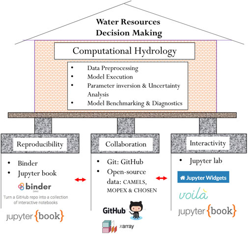
FIGURE 1. HydroBench supports computational hydrology and water resources decision making by facilitating reproducibility, collaboration, and computational interactivity. Voila is a widget rendering tool that enables interactive computation (https://github.com/voila-dashboards/voila), while Xarray is a standardized data format that eases working on multidimensional datasets (https://docs.xarray.dev/en/stable/).
Hydrological computations may require the use of more than one Jupyter Notebook or a very long single notebook. Having long or multiple notebooks leads to story fragmentation. To avoid this fragmentation, a Jupyter Book can be used to bind together multiple notebooks (Community, 2020 - https://jupyterbook.org/intro.html). A Jupyter Book is a compilation of notebooks and markdown (text) readme-files. This compilation can then be published as a traditional book narrating the computational story from its multiple components.
One way to facilitate scientific reproducibility is by openly sharing a complete, re-runnable workflow over the cloud. Binder is a web-based cloud platform that enables sharing and executing codes by recreating the computational environment without installing packages locally (Jupyter et al., 2018). Since the computational environment is recreated on the cloud, Binder makes reproducing codes and their results a single-click task. Thus, Binder not only provides a reproducible environment but also simplifies the user experience.
Collaboration is key in both model development and diagnostics. Git is a version control state-of-the art tool for code development and collaboration, while GitHub and other similar platforms are online repositories that enable sharing and collaboration on codes. Through its version-control features, Git enables a reproducible workflow among groups of collaborators on a project. In addition to collaboration on code developments, open-source hydrological data are also critical for community-wide model benchmarking, as they enable modelers to test their hypotheses beyond local watersheds and over a broad range of time against consistent information. Examples of large-sample open-source data in hydrology include the MOPEX, CAMELS, EMDNA, and CHOSEN datasets (Duan et al., 2006; Addor et al., 2017; Tang et al., 2021; Zhang et al., 2021).
The third pillar of HydroBench is interactive computation. Although sharing codes, executables and data is critical in reproducibility, codes are not always user-friendly, as their use is impossible without baseline expertise. In contrast, widgets are user-friendly tools that can be intuitively executed with clicks and slider bars. As a result, they can support most users and stakeholders across the spectrum of computing skills. In addition, widgets clear up code blocks and can facilitate interpretation through informative visualizations.
Numerous model predictive performance metrics are used in hydrological model evaluation to compare hydrological responses such as observed and modeled streamflow (and/or water table, or evapotranspiration) data. Each metric has a different skill in its evaluation. For instance, the Pearson correlation coefficient is effective in revealing the linear relationship between observed and modeled output, while the log-transformed Nash-Sutcliffe coefficient is more sensitive to low flow regimes than high flows. A detailed skills description of these metrics can be found in Krause et al. (2005), Gupta et al. (2009), and Moriasi et al. (2015). Due to their variation in skill, it is recommended to evaluate models using multiple metrics (Bennett et al., 2013). As a result, HydroBench includes multiple statistical metrics as indicators of models’ predictive performances. Table 1 provides the list of HydroBench’s model predictive performance metrics and their corresponding skills. These metrics are selected according to their skill, widespread use in hydrology, complementarity, and avoidance of redundancy. In terms of skill, they cover high and low flows, volume, and overall hydrograph characteristics (Table 1 and Figure 2).
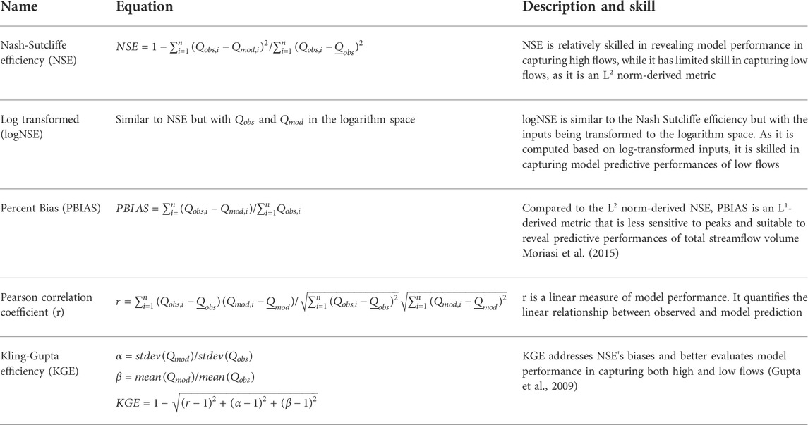
TABLE 1. List and description of predictive performance evaluation metrics in HydroBench. Here, Q represents streamflow, an example of the dependent variable, P represents precipitation, as an example of an input flux variable, mod = model, and obs = observed.
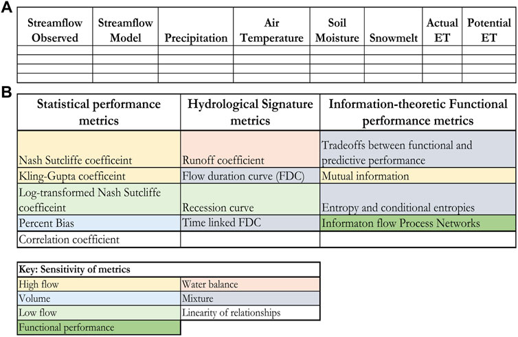
FIGURE 2. (A) Example of a standard input table to HydroBench. The empty cells refer to user provided input data, and (B) Summary of the output metrics of HydroBench and their sensitivities (color-coded). Color codes, described in the lower table (“Key: sensitivity of metrics”) indicate the hydrological feature to which the metric is most sensitive.
Statistical predictive performance metrics lack hydrological rigor and are not sufficient in diagnosing model performances (Gupta et al., 2008; McMillan, 2021). In contrast, the use of hydrological signature metrics can help diagnose model performances by indicating the model’s ability to reproduce specific hydrological processes such as high/low flows or subsurface flows. Multiple process-based signature metrics are implemented in HydroBench (Table 2). Table 2 provides a description and relative skills of the signature metrics, which are complementary to each other in characterizing subsurface flow, different segments of a hydrograph and water balance. In addition, we have also created an interface between TOSSH and HydroBench to support the full access of the TOSSH hydrological signature metrics to HydroBench users. A detailed guide of the interface is provided in the example notebook included in HydroBench. For an extended list, skill, and computation of hydrological signatures, we refer users to the TOSSH toolbox and the references therein (Gnann et al., 2021).
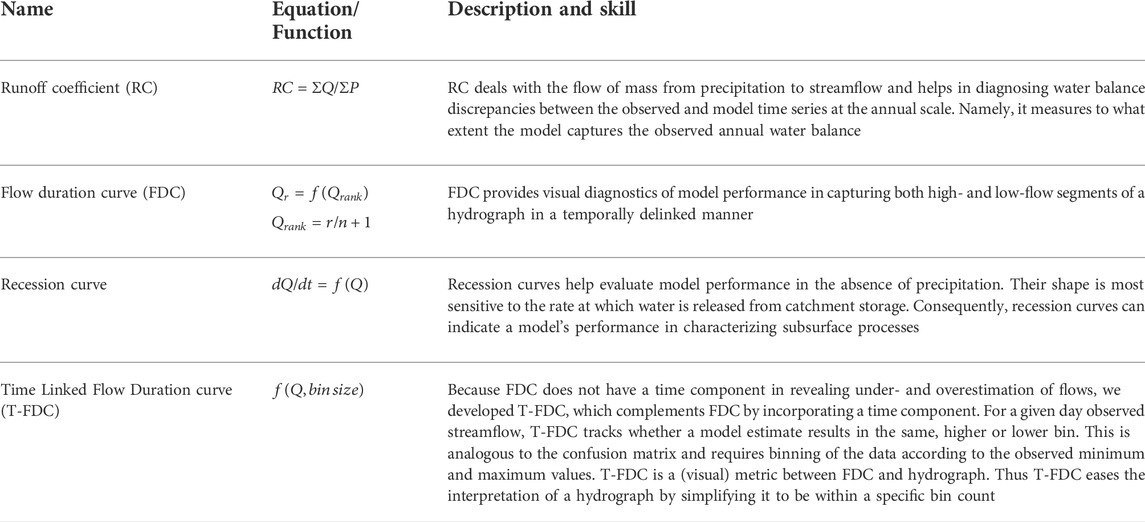
TABLE 2. List and description of hydrological signature-based model diagnostic metrics in HydroBench. Here, Q denotes streamflow, an example of the dependent variable, P denotes precipitation, an example of an input flux variable, and r denotes rank based on a decreasing sorting of a time series.
HydroBench includes Hydrograph and Flow Duration Curve (FDC) as part of the signature metrics. However, a hydrograph becomes cumbersome and difficult to interpret when the time-series being evaluated is long (i.e., multiple years of fine resolution data). Similarly, as FDC is purely probabilistic, it delinks the temporal dimension of the streamflow magnitude. That is, as long as the model preserves the exceedance probability of the observed data, FDC suggests high model performance, regardless of the time coincidence of the model simulation. Complementing the hydrograph and FDC, we developed a signature metric that is probabilistic like FDC but also preserves the time correspondence of the simulation like a hydrograph. The metric is called Time linked Flow Duration Curve (T-FDC), and it inherits the characteristics of both FDC and a hydrograph.
T-FDC is a heatmap-based model performance evaluation hydrological signature metric. In constructing the heatmap, T-FDC first lets users define a bin size for segmenting streamflow. Second, it bins the observed streamflow to the predefined bin size and sets it as the y-axis. Then, for its x-axis, T-FDC tracks whether the time corresponding model-simulated streamflow is binned in the same bin class as the observed streamflow or other bin classes. Finally, it generates a heatmap based on the time-tracked counts of the simulated streamflow in each bin class. A perfect model with a high number of data counts in the same bin as the observed values will only populate the main diagonal of the heatmap. In contrast, a high number of data counts below the diagonal indicate an underestimating model, while an overestimating model will have a high number of counts above the diagonal. This makes T-FDC's visual interpretation intuitive. In addition to the visual interpretation, we have included a numerical quantification of model performance based on T-FDC using the percentage of data counts in the diagonal. Higher percentages indicate higher performance and vice versa.
Beyond the predictive metrics and signature measures, recent developments in hydrological model diagnostics involve the use of information-theoretic metrics (Nearing et al., 2018, 2020). Compared to the predictive and hydrological signature metrics, the information-theoretic metrics require longer hydrological records. However, the diagnostic information they provide about why a model may be exhibiting poor performance, or whether it exhibits good performance for the right reasons, can be more powerful. Specifically, HydroBench provides a suite of information theoretic-based metrics (Table 3) that reveal 1) functional model performance, 2) predictive model performance and 3) the tradeoff between functional and predictive performances. Functional performance can be quantified by comparing observed transfer entropy (TE) with modeled TE and visualized using information flow process network (PN) illustrating functional relationships within the model (Ruddell et al., 2019). TE is a measure of time-lagged information flow from a “source” to a “sink” variable that accounts for autocorrelation in the “sink” time series. Unlike the runoff coefficient, which quantifies the flow of mass from precipitation (P) to streamflow (Q), PNs quantify information flow (i.e., uncertainty reduction of Q by P) between these and other variables. On the other hand, the predictive performance of a model can be quantified as the mutual information (MI) between the observed and modeled time series, which functions similarly to a correlation coefficient but is robust to nonlinearity (Ruddell et al., 2019). By providing visualizations of these metrics and how they vary across alternative models, HydroBench helps reveal the tradeoffs between predictive and functional performances.
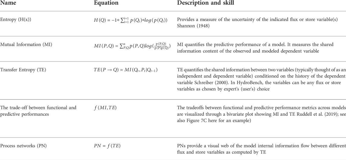
TABLE 3. List and description of information-theoretic model diagnostic metrics. Here, Q denotes streamflow, an example of the dependent variable of interest, and P denotes precipitation, an example of an input flux variable.
In HydroBench, predictive performance is quantified based on the similarity between the observed and predicted streamflow time series, computed through their mutual (i.e., shared) information (1-MI). Functional performance is evaluated as a comparison of information flows from a forcing variable (e.g., temperature, precipitation) to a sink variable (e.g., streamflow) in the model versus observations (
HydroBench additionally provides one, two and three-dimensional entropy measures for the given random variables X, Y, and Z as H(X), H(X, Y) and H(X, Y, Z), that quantify the information content of a single variable or its simultaneous interactions with multiple other variables. However, higher-dimensional quantities require longer data record lengths than the metrics discussed above. Along with their data length requirements, information theoretic metrics have a few shortcomings or caveats in comparison to the other metrics. As information theoretic metrics are dependent on probability distributions rather than on actual variable values, it is important to use them along with hydrological signatures and statistical performance measures that are a function of the actual values of the variables. Moreover, the computation of these information-theoretic metrics involves subjective parameters such as the number of bins and the statistical significance threshold. The Jupyter notebook accompanying HydroBench describes these parameters and their computation, including the number of bins and statistical significance.
HydroBench is a model-agnostic platform that requires basic Python programming skills. It can be downloaded/cloned from the following GitHub link https://github.com/EMscience/HydroBench with multiple application test cases and a particular focus on the Cedar River, WA. HydroBench accepts model and observed data in a predefined structure. The input structure is a table of data that consists of at least two data columns (e.g., observed streamflow, and model streamflow), along with their start and end dates (Figure 2). The model that generated the data can be lumped or distributed, as HydroBench requires inputs of time series variables. With these inputs, basic benchmarking results can be obtained. The basic results are the predictive performance metrics, plus FDC and T-FDC diagnostics. With an extended input table that contains one or more additional columns of independent variables (e.g., precipitation), HydroBench can provide all three types of metrics - predictive, hydrological signature, and functional (Figure 2). Since HydroBench has a modular design, it can easily be called into any notebooks that host model results and generate a table of inputs (e.g., Figure 2A). Additionally, any single metric can be employed depending on users’ preferences.
HydroBench was applied to a 103.5-km2, relatively low-gradient watershed near Cedar River, WA (Figure 3), which was extracted from the NHM infrastructure (Regan et al., 2018) for this case study. The Cedar River watershed was selected for the case study because it is considered undisturbed according to the GAGES II classification (Falcone et al., 2010) and because NHM-PRMS predictions of its streamflow strongly contrast between the calibrated and uncalibrated version of the model (Section 3). The catchment’s land cover is dominated by a coniferous forest (Falcone et al., 2010). Comparing the long-term (1980–2016) average monthly precipitation and catchment area-normalized streamflow volume, streamflow is higher than precipitation from April to July, indicating that most of the streamflow is a function of storage during these months, while the remaining months are dominated by precipitation, meaning that water enters storage. The catchment resides in a humid climate, where 53% of precipitation falls as snow (Figure 3 and Falcone et al., 2010).
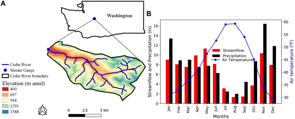
FIGURE 3. Case study watershed near Cedar River, WA: (A) location and elevation, and (B) annual hydrometeorological characteristics. The WA basemap source data is from https://geo.wa.gov/.
The model under consideration is NHM-PRMS. NHM-PRMS provides two hydrological model products based on two model parameter sets: a nationally calibrated set and the uncalibrated set (Driscoll et al., 2018; Hay, 2019). In the NHM-PRMS uncalibrated model (Driscoll et al., 2018), parameters are estimated from both catchment and climatic characteristics (Markstrom et al., 2015; Regan et al., 2018; Regan et al., 2018). In cases where estimation is impossible, the uncalibrated product is based on model default parameter values from Markstrom et al. (2015). This approach has its advantages and limitations. Primarily, it is fast compared to automatic calibration schemes and can be used to initialize the PRMS model for a further automatic calibration. Additionally, the approach might also be beneficial for parameter estimation in ungauged watersheds and nonstationary systems, as it does not rely on historical climatic/meteorological data. However, the approach becomes poor in cases where local data is sparse and in regions where the model is not tested before, as the default values may not be relevant. An extended description of the uncalibrated NHM-PRMS model parameter estimation and its product can be found at Regan et al. (2018) and Driscoll et al. (2018).
The calibrated version of NHM-PRMS employed a multivariable stepwise parameter estimation using the Shuffle Complex Evolution algorithm (Hay and Umemoto, 2007; Hay et al., 2006 & 2019). In starting the calibration, the parameters were initialized at their uncalibrated NHM-PRMS value. The calibration uses multiple variables, including daily streamflow from 1980 to 2010 and for the same period, monthly snow cover area (SCA, from SNODAS; National Operational Hydrologic Remote Sensing Center, 2004), potential evapotranspiration and solar radiation (PET and SR, from Farnsworth and Thompson, 1982, the DAYMET climate data and Regan et al., 2018), actual evapotranspiration (AET, from Cao et al., 2006; Rietjes et al., 2013) and soil moisture estimates (SM, from Campo et al., 2006; Thorstensen et al., 2016). These data are derived from national scale remotely sensed datasets and other model products. The sensitivity of the different model parameters to these variables is assessed, and parameters are then sequentially calibrated with an objective function defined as the normalized root mean square error between the observed and simulated values of the output variables in decreasing order of sensitivity (Markstrom et al., 2016). That is, in calibrating PRMS to these variables, sensitivity analysis guides the identification of which parameters are calibrated by which variable in a stepwise manner. Stepwise calibration starts with 1) PET and SR, followed by 2) SM and AET, and finally, 3) streamflow. For a detailed description of the model calibration and the optimization employed, please refer to Hay et al. (2006), Hay and Umemoto (2007) and LaFontaine et al. (2019).
In demonstrating the application of HydroBench at the Cedar River, we evaluated model performance with respect to the input, state, and output variables of the calibrated and uncalibrated NHM-PRMS model. Namely, as NHM-PRMS computes hydrologic fluxes using inputs of daily precipitation and maximum and minimum air temperature, these variables were included in our analysis. Similarly, we extracted the predicted variables of streamflow, snowmelt, basin soil moisture, and actual evapotranspiration from 1980 to 2016 at a daily time step for our model benchmarking and diagnostics at the Cedar River, WA.
Facilitating reproducibility, all inputs and the results presented in this section are available on GitHub (https://github.com/EMscience/HydroBench). As a Binder link is also included, the analysis can be fully reproduced, and the different widgets can also be used for further interactive computation on the cloud. Thus, users of HydroBench can emulate and adapt the workflow easily.
At the Cedar River watershed, the uncalibrated model shows better statistical predictive performance than the calibrated model, according to the HydroBench-provided statistics, except for the KGE metric under the log-transformed flow condition (Table 4 and Figure 4). Regardless of the skills of the metrics in representing the different hydrograph segments (low or high flows), most of the predictive performance metrics suggest that the uncalibrated model is a preferred choice (Tables 1–3). However, the predictive performance metrics do not explain why and how the uncalibrated model exhibits better predictive performance than the calibrated model. In addition, it is important to note that the calibration of NHM-PRMS does not only focus on the prediction of streamflow but also on capturing remotely sensed ET and other variables with a stepwise calibration method.

TABLE 4. Summary of statistical predictive performance metrics for the uncalibrated and calibrated NHM-PRMS model of a watershed near Cedar River, WA, based on daily streamflow, 1980–2016.
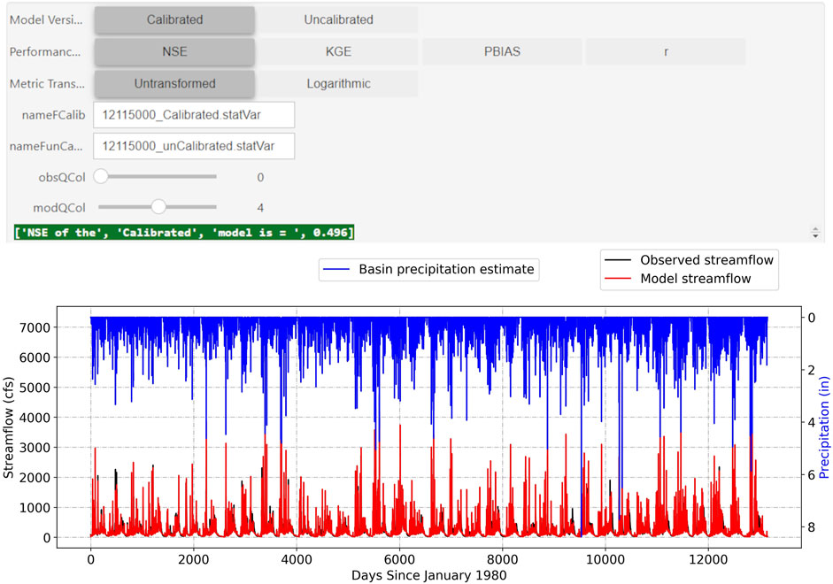
FIGURE 4. Screenshot of HydroBench interactive window showing predictive performance metrics and the corresponding hydrograph for NHM-PRMS simulations of the Cedar River watershed daily streamflow, 1980–2016, compared to observations (USGS stream gage, 12115000).
Both the FDC and T-FDC indicate that high flows are better represented by the uncalibrated model (Figures 5A, 6; Table 5). In contrast, the recession curves indicate that the subsurface release of water from storage over extended periods is better represented by the calibrated model (Figures 5C,D; Table 5), as it has a scatter (slope and intercept) more similar to the observations than does the partly near-linear (in a semi-log space) uncalibrated model. Figure 6 along with Table 5 shows that the calibrated model is closely related to the observed data (35% than 33%). On the other hand, the runoff coefficient (RC) comparison between both model versions indicates strong similarity between the models, with an RC model to RC observed ratio of 0.969 for the calibrated and 1.003 for the uncalibrated model (Figure 5B). The similarity in RC may suggest that the annual mass flow (precipitation to streamflow) of the two models is similar, with slightly more precipitation converted into streamflow in the uncalibrated model.

TABLE 5. Numerical scores of hydrological signature metrics. For this test case, we chose the mid slope of the FDC (25–45% exceedance probability). Similarly, we chose the main diagonal in T-FDC as a strict measure and ‘Dry’ months (April—September) for recession score as a representative of subsurface flow dominant season. HydroBench allows users to choose the exceedance probabilities, the number of diagonals in T-FDC and seasons for recession curve scores.
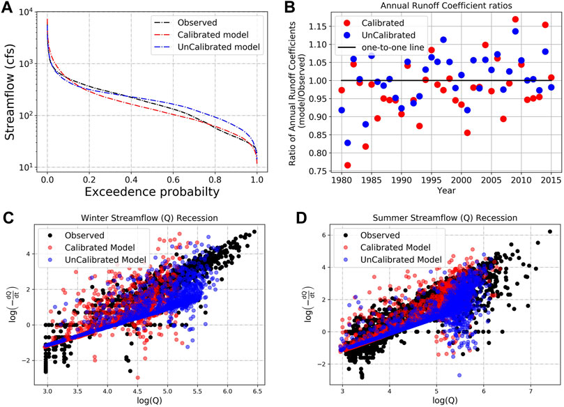
FIGURE 5. Hydrological signature-based evaluation of NHM-PRMS predictions of daily streamflow at Cedar River, WA over 1980–2016: (A) flow duration curve, (B) annual (i.e., October to September water year) runoff coefficient, (C) winter/cold season (months October to March) recession curves and, (D) summer/warm season (months April to September) recession curves. The seasons and the corresponding months can be adaptively defined in HydroBench.
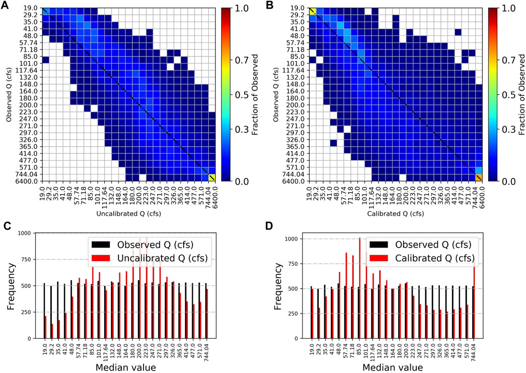
FIGURE 6. Time-linked flow duration curve for (A) the uncalibrated model and (B) the calibrated model (C) the sum of the number of simulated flows in the same flow range bin as the observed for the uncalibrated model and (D) the same as C but for the calibrated model. Figures (A,B) show how the observed flows in each bin are distributed across the bins of the model estimated flows. The number of bins, a user-defined value, is 25 here. Ideally, hot colors would populate the diagonal, implying minimum over/underestimations.
Despite the high statistical predictive performance reports of the uncalibrated model (Table 4), the hydrological signature metrics revealed that the calibrated model better represents the low-flow segments of the Cedar River hydrograph. This comparison of predictive and hydrological signature metrics underscores the need for both types of performance evaluations. Although hydrological process signature metrics illuminate the failure or success of each model in representing different processes, neither they nor the statistical predictive metrics can reveal what type of model input and output interactions lead to the model results, underscoring the need for functional performance evaluations.
The calibrated and uncalibrated models have a similar pattern of information flows, depicted in their process networks (PN), with a few exceptions (Figures 7A,B; Table 6). For example, the PNs depict high transfer entropy (TE) from precipitation to snowmelt in the uncalibrated model. In contrast, the calibrated model has high TE from precipitation directly to streamflow. Although observations of daily snowmelt are not available for this watershed for comparison to an observed PN, the PN difference noted by the models suggests that snowmelt contributions in the uncalibrated model could be the cause of low flow overestimation in the FDC. Following these insights from the PN plots, we explored the day of the year (DoY) averages, minimums and maximums of snowmelt, actual evapotranspiration and soil moisture of the two models (Figure 8). The figure showed that the uncalibrated model leads to snowmelt processes even in the late summer months, which is not likely.
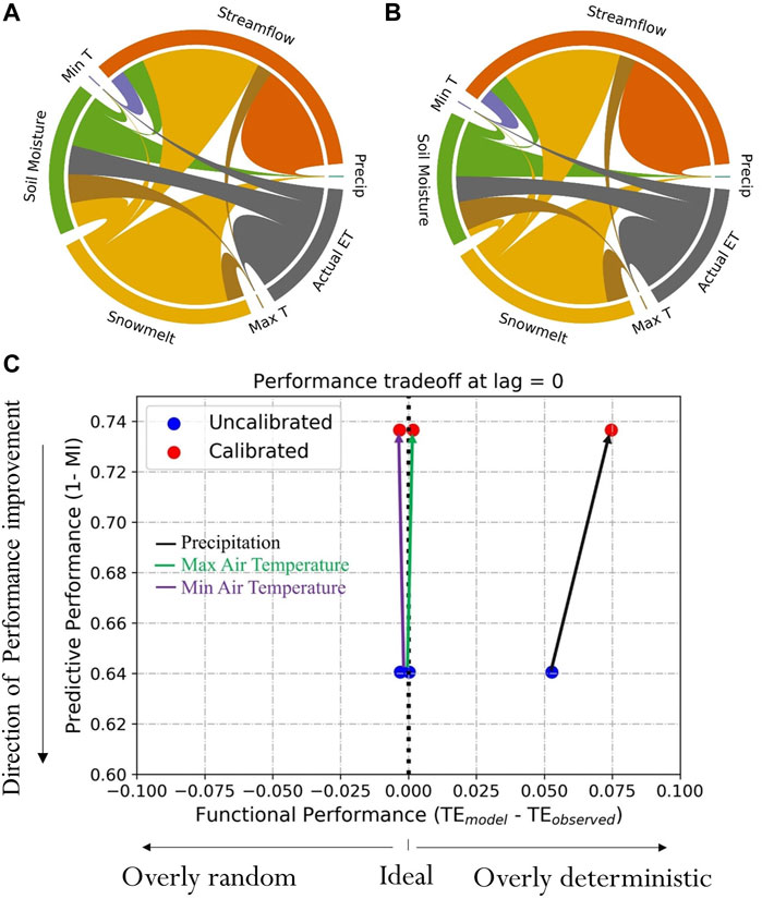
FIGURE 7. Functional performance metrics based on evaluation of NHM-PRMS at the Cedar River watershed. (A) uncalibrated model and (B) calibrated model, and (C) tradeoff between functional and predictive performance metrics. In interpreting PN plots, the outer colored circle indicates the interacting variables. The width of the chords linking the interacting variables corresponds to the TE magnitudes. In (C), the change in predictive performance and functional performance from the uncalibrated model (origin of the arrow, blue) to the calibrated model (point of the arrow, red) is plotted. Thus, the arrows show the effect of calibration. The difference between the two figures is presented in Table 6.
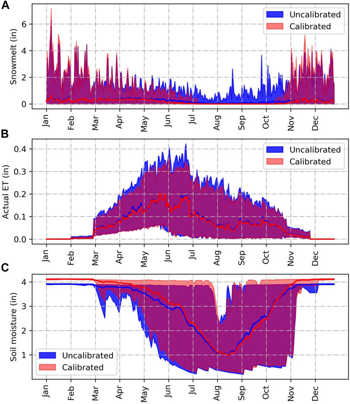
FIGURE 8. Day of the year averages of (A) snowmelt, (B) actual evapotranspiration and (C) soil moisture for both the calibrated and uncalibrated model.
The visualization of tradeoffs between predictive and functional performance metrics (Figure 7C) shows that calibration decreased the predictive performance of the model, primarily by over-extracting information from precipitation to inform streamflow (as seen in the higher transfer entropy from precipitation to model streamflow, i.e.,
Overall, HydroBench showed that the calibrated and uncalibrated NHM-PRMS model products at the Cedar River watershed have different skills. Although long-term snow and moisture observational data were not available to support the diagnosis of performance discrepancies, HydroBench produced a set of insights into the mechanisms underlying performance differences. In summary, the uncalibrated model exhibited better statistical predictive performance than the calibrated model, particularly during high flows. However, the uncalibrated model was less skilled at capturing low flows and streamflow recession processes, based on the hydrological signature metrics. Functional metrics suggested that routing of precipitation through snow storage and melt differs between the two models, with the calibrated model abstracting too much information directly from precipitation. Thus, it is likely that the uncalibrated model does a better job of capturing peak flows than the calibrated model because it better represents the initial release of water from the snowpack. However, the tradeoff is that the release of water from storage from the uncalibrated simulation is too high during baseflow-dominated periods, in comparison to the calibrated model.
In general, information about whether the relationship between variables is overly random or overly deterministic, as in the Cedar River, can provide useful insight into the next steps. In an overly-random system, although the process information is contained in the observations, it is under-utilized, meaning the model might not have extracted it effectively. Structural changes to the model to represent hydrologic processes more realistically, a better calibration strategy, and/or better objective function may help extract the process information contained in the observations. In contrast, in an overly-deterministic system where there is ‘over extraction’, it might be better to reduce the dependency of the model on the observed input data. The reduction in dependency might be achieved through diversifying the input data by, for example, incorporating new data (e.g., adding snow and soil moisture data into a model that was forced by precipitation and temperature inputs). Additionally, the user may consider changing the model optimization strategy. Alternative strategies may include calibrating and validating the model in contrasting seasons and hydrograph regimes, using transformed data, and/or changing calibration and validation objective functions in a way that penalizes models in which training data have substantially higher performance than test data. These approaches may lead to less reliance of the model on specific variables or aspects of a variable that have resulted in the overly-deterministic fit.
For the Cedar River case study, the insight provided by HydroBench suggests that further calibration would be a logical next step. Though the calibrated model exhibited poorer predictive performance, its improved ability to capture low flow dynamics may indicate that performance gains can be obtained without changing the model structure. The parameters of focus may be those relevant to snow and soil storage, and the objective function of the calibration may need to be adjusted further to upweight peak flows. Alternatively, the tradeoff in better low-flow performance at the expense of high-flow performance seen in the calibrated model may suggest that rather than an ‘absolute best model’ parameter set, there exists a Pareto front (i.e., an unavoidable tradeoff). However, this possibility would need to be tested using a multi-objective optimization scheme for calibration that provides the Pareto front. Finally, if further parameter calibration attempts failed to improve the predictive performance of the model while maintaining acceptable functional performance, the modeler may wish to revisit the fundamental structure (i.e., equations) of the model. In this case, the representation of snow storage and melt processes in PRMS might need to be revised to better reflect the Cedar River catchment response.
Alternatively, given the two tested models, a user may decide to opt for the uncalibrated model if most interested in outcomes related to high flows, or the calibrated model if most interested in low flows. Additionally, users or developers may decide to adopt model averaging techniques such as Bayesian Model Averaging -or Hierarchical Mixture of Experts to derive a consensus prediction (Marshall et al., 2006; Duan et al., 2007; Moges et al., 2016). Importantly, the application of HydroBench to the test case proves that relying only on high performance statistical predictive measures can be misleading as shown by the high predictive performance but the poor functional performance of the uncalibrated model. Thus, a holistic performance evaluation is critical.
Model benchmarking and diagnostics are not only at the core of model trust and reliability but also serve as guides for future model development and improvements. HydroBench was designed as a model diagnostic and benchmarking tool in a practice of open, reproducible science. The tool relies on the Jupyter ecosystem for reproducible, collaborative, and interactive computation. HydroBench enables model performance evaluation and diagnosis of performance discrepancies by providing three sets of complementary metrics, including statistical performance metrics, process-based hydrological signatures, and information theoretic-based tools. As demonstrated in the test case, this tool produces insight into many different aspects of a model’s performance and helps diagnose performance shortfalls.
The metrics in HydroBench support the different aspects of model evaluation outlined in Gleeson et al. (2021), including a comparison of model results against 1) observations, 2) other models, and/or 3) expert-based expectations. All of the metric categories in HydroBench (predictive, process diagnostics, and functional performances) facilitate comparison against observations in watersheds that have observed data. The information theoretic-based model functional performance metric using PN supports model comparisons even in the absence of observed data, though availability of observed data strengthens such comparisons (e.g., Figures 7A,B). Similarly, PNs and the hydrological signatures can facilitate expert-based model evaluation as they highlight the key hydrological processes and model hypotheses. The graphical representation of a PN can be interpreted as an imprint of the models’ process conceptualization. HydroBench can be used to formalize and standardize the ad-hoc expert-based model evaluation approaches commonly applied by the hydrologic science community.
Although all the three categories of metrics in HydroBench are designed to be used in concert, HydroBench is modular and supports the use of any of the metrics individually. For instance, in watersheds with abundant data, all capabilities of HydroBench can be utilized. However, in cases of limited record length or data diversity, a user may decline to use information-theoretic metrics because they are not reliable in limited record lengths.
Choice of calibration objective functions dictates model performance and sensitivity analysis results (Diskin and Simon, 1977; Jie et al., 2016; Markstrom et al., 2016; Garcia et al., 2017). For instance, a model calibrated using root mean square error may not result in better performance in logNSE. Thus, in using HydroBench, we suggest a careful choice of performance metrics that reflect the modeling objective. For instance, for pure predictive purposes, such as short term flow forecasts, relying on predictive performance metrics is beneficial. On the other hand, water balance projections and quantifications can better be served by signature based diagnostics and functional performance evaluation metrics as they seek to get the right answer for the right reasons. Furthermore, in modeling works that start with a sensitivity analysis, the sensitivity analysis result can also be used to align sensitive parameters, modeling objectives and evaluation metrics. That is, evaluating models based on a metric that reflects the objective function set for the sensitivity analysis. Although this approach is consistent with the user’s modeling objective, the approach is susceptible to getting the right answer for the wrong reasons. For instance, in a non-stationary system, an insensitive parameter or process can be activated and the prediction and evaluations can be misplaced. In this regard, multi-objective calibration and comprehensive model evaluation across the three categories of HydroBench can be beneficial in diagnosing whether the model is right for the right reasons.
In addition to its utility in hydrologic research and applications, HydroBench can be used to support hydrological teaching that focuses on modeling and model evaluations (Wagener and Mcintyre, 2007; Wagener et al., 2012). Last, HydroBench is an open source project and can be extended by the community and also integrated with other benchmarking tools, as TOSSH is interfaced with HydroBench.
The datasets presented in this study can be found in online repositories. The names of the repository/repositories and accession number(s) can be found below: https://github.com/EMscience/HydroBench, and https://zenodo.org/badge/latestdoi/375593287.
EM, BR, FP, JD, and LL: motivation and framing of the work. EM: first draft manuscript development and writing. BR: MatLab code for the Information theory metrics which was translated to Python by EM. PN and JD: dataset for NHM-PRMS. All authors: discussions, manuscript editing and improvements.
This work is partially supported by the U.S. Geological Survey Powell Center for Analysis and Synthesis, a Gordon and Betty Moore Foundation Data-Driven Discovery Investigator grant to LL, and the Jupyter Meets the Earth project, funded by NSF grant numbers 1928406 and 1928374 to LL and FP.
Any use of trade, firm, or product names is for descriptive purposes only and does not imply endorsement by the U.S. Government.
The authors declare that the research was conducted in the absence of any commercial or financial relationships that could be construed as a potential conflict of interest.
All claims expressed in this article are solely those of the authors and do not necessarily represent those of their affiliated organizations, or those of the publisher, the editors and the reviewers. Any product that may be evaluated in this article, or claim that may be made by its manufacturer, is not guaranteed or endorsed by the publisher.
Addor, N., and Melsen, L. A. (2019). Legacy, rather than adequacy, drives the selection of hydrological models. Water Resour. Res. 55, 378–390. doi:10.1029/2018WR022958
Addor, N., Newman, A. J., Mizukami, N., and Clark, M. P. (2017). The CAMELS data set: Catchment attributes and meteorology for large-sample studies. Hydrol. Earth Syst. Sci. 21, 5293–5313. doi:10.5194/hess-21-5293-2017
Bennett, A., Nijssen, B., Ou, G., Clark, M., and Nearing, G. (2019). Quantifying process connectivity with transfer entropy in hydrologic models. Water Resour. Res. 55, 4613–4629. doi:10.1029/2018WR024555
Bennett, N. D., Croke, B. F. W., Guariso, G., Guillaume, J. H. A., Hamilton, S. H., Jakeman, A. J., et al. (2013). Characterising performance of environmental models. Environ. Model. Softw. 40, 1–20. doi:10.1016/J.ENVSOFT.2012.09.011
Campo, L., Caparrini, F., and Castelli, F. (2006). Use of multi-platform, multi-temporal remote-sensing data for calibration of a distributed hydrological model: An application in the arno basin, Italy. Hydrol. Process. 20, 2693–2712. doi:10.1002/HYP.6061
Caol, W., Sun, G., Chen, J., Noormets, A., and Skaggs, R. W. (2006). Evapotranspiration of a Mid-Rotation Loblolly Pine Plantation and a Recently Harvested Stands on the Coastal Plain of North Carolina, U.S.A. Williams, Thomas, eds. Hydrol. Manag. For. Wetl. Proc. Int. Conf. St. Joseph, MI Am. Soc. Agric. Biol. Eng. 27-33.
Clark, M. P., Rupp, D. E., Woods, R. A., Tromp-van Meerveld, H. J., Peters, N. E., and Freer, J. E. (2009). Consistency between hydrological models and field observations: Linking processes at the hillslope scale to hydrological responses at the watershed scale. Hydrol. Process. 23, 311–319. doi:10.1002/hyp.7154
Cohen, S., Praskievicz, S., and Maidment, D. R. (2018). Featured collection introduction: National water model. J. Am. Water Resour. Assoc. 54, 767–769. doi:10.1111/1752-1688.12664
De Boer-Euser, T., Bouaziz, L., De Niel, J., Brauer, C., Dewals, B., Drogue, G., et al. (2017). Looking beyond general metrics for model comparison – lessons from an international model intercomparison study. Hydrol. Earth Syst. Sci. 21, 423–440. doi:10.5194/hess-21-423-2017
Diskin, M. H., and Simon, E. (1977). A procedure for the selection of objective functions for hydrologic simulation models. J. Hydrol. X. J34, 129–149. doi:10.1016/0022-1694(77)90066-X
Driscoll, J. M., Regan, R. S., Markstrom, S. L., and Hay, L. E. (2018). Application of the national hydrologic model infrastructure with the precipitation-runoff modeling system (NHM-PRMS), uncalibrated version. U.S. Geol. Surv. doi:10.5066/P9USHPMJ
Duan, Q., Ajami, N. K., Gao, X., and Sorooshian, S. (2007). Multi-model ensemble hydrologic prediction using Bayesian model averaging. Adv. Water Resour. 30, 1371–1386. doi:10.1016/j.advwatres.2006.11.014
Duan, Q., Schaake, J., Andréassian, V., Franks, S., Goteti, G., Gupta, H. V., et al. (2006). Model Parameter Estimation Experiment (MOPEX): An overview of science strategy and major results from the second and third workshops. J. Hydrol. X. 320, 3–17. doi:10.1016/j.jhydrol.2005.07.031
Falcone, J. A., Carlisle, D. M., Wolock, D. M., and Meador, M. R. (2010). Gages: A stream gage database for evaluating natural and altered flow conditions in the conterminous United States. Ecology 91, 621. doi:10.1890/09-0889.1
Farnsworth, R. K., and Thompson, E. S. (1982). Mean monthly, seasonal, and annual pan evaporation for the United States: Washington, D.C., National Oceanic and Atmospheric Administration Technical Report NWS 34, 82 p
Garcia, F., Folton, N., and Oudin, L. (2017). Which objective function to calibrate rainfall–runoff models for low-flow index simulations? Hydrological Sci. J. 62 (7), 1149–1166. doi:10.1080/02626667.2017.1308511
Gil, Y., David, C. H., Demir, I., Essawy, B. T., Fulweiler, R. W., Goodall, J. L., et al. (2016). Toward the Geoscience Paper of the Future: Best practices for documenting and sharing research from data to software to provenance. Earth Space Sci. 3, 388–415. doi:10.1002/2015EA000136
Gleeson, T., Wagener, T., Döll, P., Zipper, S. C., West, C., Wada, Y., et al. (2021). GMD perspective: The quest to improve the evaluation of groundwater representation in continental-to global-scale models. Geosci. Model Dev. 14, 7545–7571. doi:10.5194/GMD-14-7545-2021
Gnann, S. J., Coxon, G., Woods, R. A., Howden, N. J. K., and McMillan, H. K. (2021). Tossh: A toolbox for streamflow signatures in hydrology. Environ. Model. Softw. 138, 104983. doi:10.1016/J.ENVSOFT.2021.104983
Gupta, H. V., Kling, H., Yilmaz, K. K., and Martinez, G. F. (2009). Decomposition of the mean squared error and NSE performance criteria: Implications for improving hydrological modelling. J. Hydrol. X. 377, 80–91. doi:10.1016/j.jhydrol.2009.08.003
Gupta, H. V., Wagener, T., and Liu, Y. (2008). Reconciling theory with observations: Elements of a diagnostic approach to model evaluation. Hydrol. Process. 22, 3802–3813. doi:10.1002/hyp.6989
Hallouin, T. (2021). hydroeval: an evaluator for streamflow time series in Python. Zenodo. doi:10.5281/ZENODO.4709652
Hay, L. (2019). Application of the national hydrologic model infrastructure with the precipitation-runoff modeling system (NHM-PRMS), by HRU calibrated version - ScienceBase-catalog. U.S. Geol. Surv. Available at: doi:10.5066/P9NM8K8WAccessed February 23, 2022)
Hay, L. E., Leavesley, G. H., Clark, M. P., Markstrom, S. L., Viger, R. J., and Umemoto, M. (2006). Step wise, multiple objective calibration of a hydrologic model for a snowmelt dominated basin. J. Am. Water Resour. Assoc. 42, 877–890. doi:10.1111/J.1752-1688.2006.TB04501.X
Hay, L. E., and Umemoto, M. (2007). Multiple-objective stepwise calibration using luca. Available at: http://www.usgs.gov/pubprod [Accessed June 7, 2022].
Hutton, C., Wagener, T., Freer, J., Han, D., Duffy, C., and Arheimer, B. (2016). Most computational hydrology is not reproducible, so is it really science? Water Resour. Res. 52, 7548–7555. doi:10.1002/2016WR019285
Jie, M. X., Chen, H., Xu, C. Y., Zeng, Q., and Tao, X. E. (2016). A comparative study of different objective functions to improve the flood forecasting accuracy. Hydrology Res. 47, 718–735. doi:10.2166/NH.2015.078
Jupyter, P., Bussonnier, M., Forde, J., Freeman, J., Granger, B., Head, T., et al. (2018). Binder 2.0 - reproducible, interactive, sharable environments for science at scale. Proceedings of the 17th Python in Science Conference, July 9-15, 2018 Austin, Texas, 113–120. doi:10.25080/MAJORA-4AF1F417-011
Kirchner, J. W. (2009). Catchments as simple dynamical systems: Catchment characterization, rainfall-runoff modeling, and doing hydrology backward. Water Resour. Res. 45, n/a. doi:10.1029/2008WR006912
Kirchner, J. W. (2006). Getting the right answers for the right reasons: Linking measurements, analyses, and models to advance the science of hydrology. Water Resour. Res. 42, n/a. doi:10.1029/2005WR004362
Kollet, S., Sulis, M., Maxwell, R. M., Paniconi, C., Putti, M., Bertoldi, G., et al. (2017). The integrated hydrologic model intercomparison project, IH-MIP2: A second set of benchmark results to diagnose integrated hydrology and feedbacks. Water Resour. Res. 53, 867–890. doi:10.1002/2016WR019191
Krause, P., Boyle, D. P., and Bäse, F. (2005). Comparison of different efficiency criteria for hydrological model assessment. Adv. Geosci. 5, 89–97. Available at: doi:10.5194/adgeo-5-89-2005https://hal.archives-ouvertes.fr/hal-00296842/(Accessed February 27, 2015)
LaFontaine, J. H., Hart, R. M., Hay, L. E., Farmer, W. H., Bock, A. R., Viger, R. J., et al. (2019). Simulation of water availability in the Southeastern United States for historical and potential future climate and land-cover conditions. Sci. Investig. Rep. 2019–5039, 83 doi:10.3133/SIR20195039
Lane, R., Coxon, G., E Freer, J., Wagener, T., J Johnes, P., P Bloomfield, J., et al. (2019). Benchmarking the predictive capability of hydrological models for river flow and flood peak predictions across over 1000 catchments in Great Britain. Hydrol. Earth Syst. Sci. 23, 4011–4032. doi:10.5194/HESS-23-4011-2019
Markstrom, S. L., Hay, L. E., and Clark, M. P. (2016). Towards simplification of hydrologic modeling: Identification of dominant processes. Hydrol. Earth Syst. Sci. Discuss., 20–4655-4671. doi:10.5194/hess-2015-508
Markstrom, S. L., Regan, R. S., Hay, L. E., Viger, R. J., Webb, R. M. T., Payn, R. A., et al. (2015). PRMS-IV, the precipitation-runoff modeling system, version 4. Available at: https://pubs.usgs.gov/tm/6b7/[Accessed September 5, 2017].
Marshall, L., Sharma, A., and Nott, D. (2006). Modeling the catchment via mixtures: Issues of model specification and validation. Water Resour. Res. 42, 11409. doi:10.1029/2005WR004613
McMillan, H. K. (2021). A review of hydrologic signatures and their applications. WIREs Water 8, e1499. doi:10.1002/WAT2.1499
McMillan, H. K., Clark, M. P., Bowden, W. B., Duncan, M., and Woods, R. A. (2011). Hydrological field data from a modeller’s perspective: Part 1. Diagnostic tests for model structure. Hydrol. Process. 25, 511–522. doi:10.1002/hyp.7841
McMillan, H. (2020). Linking hydrologic signatures to hydrologic processes: A review. Hydrol. Process. 34, 1393–1409. doi:10.1002/HYP.13632
Moges, E., Demissie, Y., and Li, H.-Y. (2016). Hierarchical mixture of experts and diagnostic modeling approach to reduce hydrologic model structural uncertainty. Water Resour. Res. 52, 2551–2570. doi:10.1002/2015WR018266
Moges, E., Ruddell, B. L., Zhang, L., Driscoll, J. M., and Larsen, L. G. (2022). Strength and memory of precipitation’s control over streamflow across the conterminous United States. Water Resour. Res. 58, e2021WR030186. doi:10.1029/2021WR030186
Moriasi, D. N., Gitau, M. W., Pai, N., Daggupati, P., Gitau, M. W., Member, A., et al. (2015). Hydrologic and water quality models: Performance measures and evaluation criteria. Trans. ASABE 58, 1763–1785. doi:10.13031/TRANS.58.10715
National Operational Hydrologic Remote Sensing Center (2004). Snow Data Assimilation System (SNODAS) Data Products at NSIDC, Version 1. Boulder, Colorado USA: NSIDC: National Snow and Ice Data Center. doi:10.7265/N5TB14TC
Nearing, G. S., Ruddell, B. L., Bennett, A. R., Prieto, C., and Gupta, H. V. (2020). Does information theory provide a new paradigm for Earth science? Hypothesis testing. Water Resour. Res. 56, e2019WR024918. doi:10.1029/2019WR024918
Nearing, G. S., Ruddell, B. L., Clark, M. P., Nijssen, B., and Peters-Lidard, C. (2018). Benchmarking and process diagnostics of land models. J. Hydrometeorol. 19, 1835–1852. doi:10.1175/JHM-D-17-0209.1
Pechlivanidis, I. G., Jackson, B., McMillan, H., and Gupta, H. (2014). Use of an entropy-based metric in multiobjective calibration to improve model performance. Water Resour. Res. 50, 8066–8083. doi:10.1002/2013WR014537
Pechlivanidis, I. G., Jackson, B., and Mcmillan, H. (2010). “The use of entropy as a model diagnostic in rainfall-runoff modelling,” in International Congress on Environmental Modelling and Software, July 5-8, 2010, Ottawa, Canada. Available at: http://www.iemss.org/iemss2010/index.php?n=Main.Proceedings (Accessed February 23, 2022).
Peñuela, A., Hutton, C., and Pianosi, F. (2021). An open-source package with interactive Jupyter Notebooks to enhance the accessibility of reservoir operations simulation and optimisation. Environ. Model. Softw. 145, 105188. doi:10.1016/J.ENVSOFT.2021.105188
Pérez, F., and Granger, B. E. (2007). IPython: A system for interactive scientific computing. Comput. Sci. Eng. 9, 21–29. doi:10.1109/MCSE.2007.53
Project Jupyter 2022 | Home Available at: https://jupyter.org/[Accessed February 24, 2022].
Regan, R. S., Juracek, K. E., Hay, L. E., Markstrom, S. L., Viger, R. J., Driscoll, J. M., et al. (2019). The U. S. Geological Survey National Hydrologic Model infrastructure: Rationale, description, and application of a watershed-scale model for the conterminous United States. Environ. Model. Softw. 111, 192–203. doi:10.1016/j.envsoft.2018.09.023
Regan, R. S., Markstrom, S. L., Hay, L. E., Viger, R. J., Norton, P. A., Driscoll, J. M., et al. (2018). Description of the national hydrologic model for use with the precipitation-runoff modeling system (PRMS). Tech. Methods 6, 38. doi:10.3133/tm6B9
Rientjes, T. H. M., Muthuwatta, L. P., Bos, M. G., Booij, M. J., and Bhatti, H. A. (2013). Multi-variable calibration of a semi-distributed hydrological model using streamflow data and satellite-based evapotranspiration. J. Hydrol. X. 505, 276–290. doi:10.1016/J.JHYDROL.2013.10.006
Ruddell, B. L., Drewry, D. T., and Nearing, G. S. (2019). Information theory for model diagnostics: Structural error is indicated by trade-off between functional and predictive performance. Water Resour. Res. 55, 6534–6554. doi:10.1029/2018WR023692
Ruddell, B. L., and Kumar, P. (2009). Ecohydrologic process networks: 1. Identification. Water Resour. Res. 45. doi:10.1029/2008WR007279
Rule, A., Birmingham, A., Zuniga, C., Altintas, I., Huang, S. C., Knight, R., et al. (2019). Ten simple rules for writing and sharing computational analyses in Jupyter Notebooks. PLOS Comput. Biol. 15, e1007007. doi:10.1371/JOURNAL.PCBI.1007007
Sandve, G. K., Nekrutenko, A., Taylor, J., and Hovig, E. (2013). Ten simple rules for reproducible computational research. PLOS Comput. Biol. 9, e1003285. doi:10.1371/JOURNAL.PCBI.1003285
Saxe, S., Farmer, W., Driscoll, J., and Hogue, T. S. (2021). Implications of model selection: A comparison of publicly available, conterminous US-extent hydrologic component estimates. Hydrol. Earth Syst. Sci. 25, 1529–1568. doi:10.5194/HESS-25-1529-2021
Schreiber, T. (2000). Measuring information transfer. Phys. Rev. Lett. 85, 461–464. doi:10.1103/PhysRevLett.85.461
Shannon, C. E. (1948). A mathematical theory of communication. Bell Syst. Tech. J. 27, 379–423. doi:10.1002/j.1538-7305.1948.tb01338.x
Stagge, J. H., Rosenberg, D. E., Abdallah, A. M., Akbar, H., Attallah, N. A., and James, R. (2019). Assessing data availability and research reproducibility in hydrology and water resources. Sci. Data 61 (6), 190030–190112. doi:10.1038/sdata.2019.30
Tang, G., Clark, M. P., Papalexiou, S. M., Newman, A. J., Wood, A. W., Brunet, D., et al. (2021). Emdna: An ensemble meteorological dataset for North America. Earth Syst. Sci. Data 13, 3337–3362. doi:10.5194/ESSD-13-3337-2021
Thorstensen, A., Nguyen, P., Hsu, K., and Sorooshian, S. (2016). Using densely distributed soil moisture observations for calibration of a hydrologic model. J. Hydrometeorol. 17, 571–590. doi:10.1175/JHM-D-15-0071.1
Tian, F., Li, H., and Sivapalan, M. (2012). Model diagnostic analysis of seasonal switching of runoff generation mechanisms in the Blue River basin, Oklahoma. J. Hydrol. X. 418–419, 136–149. doi:10.1016/j.jhydrol.2010.03.011
Tijerina, D., Condon, L., FitzGerald, K., Dugger, A., O’Neill, M. M., Sampson, K., et al. (2021). Continental hydrologic intercomparison project, phase 1: A large-scale hydrologic model comparison over the continental United States. Water Resour. Res. 57, e2020WR028931. doi:10.1029/2020WR028931
Wagener, T., Kelleher, C., Weiler, M., McGlynn, B., Gooseff, M., Marshall, L., et al. (2012). It takes a community to raise a hydrologist: The Modular Curriculum for Hydrologic Advancement (MOCHA). Hydrol. Earth Syst. Sci. 16, 3405–3418. doi:10.5194/HESS-16-3405-2012
Wagener, T., and Mcintyre, N. (2007). Tools for teaching hydrological and environmental modeling. Comput. Educ. J. 17 (3).
Weijs, S. V., Schoups, G., and van de Giesen, N. (2010). Why hydrological predictions should be evaluated using information theory. Hydrol. Earth Syst. Sci. 14, 2545–2558. doi:10.5194/hess-14-2545-2010
Yilmaz, K. K., Gupta, H. V., and Wagener, T. (2008). A process-based diagnostic approach to model evaluation: Application to the NWS distributed hydrologic model. Water Resour. Res. 44, n/a. doi:10.1029/2007WR006716
Keywords: Hydrological Modeling, Model Evaluation, Model Benchmarking, Model Diagnostics, Uncertainty Analysis, Nash Sutcliffe, Kling-Gupta, Reproducibility
Citation: Moges E, Ruddell BL, Zhang L, Driscoll JM, Norton P, Perez F and Larsen LG (2022) HydroBench: Jupyter supported reproducible hydrological model benchmarking and diagnostic tool. Front. Earth Sci. 10:884766. doi: 10.3389/feart.2022.884766
Received: 27 February 2022; Accepted: 26 July 2022;
Published: 30 September 2022.
Edited by:
Anneli Guthke, University of Stuttgart, GermanyReviewed by:
Laurene Bouaziz, Deltares, NetherlandsCopyright © 2022 Moges, Ruddell, Zhang, Driscoll, Norton, Perez and Larsen. This is an open-access article distributed under the terms of the Creative Commons Attribution License (CC BY). The use, distribution or reproduction in other forums is permitted, provided the original author(s) and the copyright owner(s) are credited and that the original publication in this journal is cited, in accordance with accepted academic practice. No use, distribution or reproduction is permitted which does not comply with these terms.
*Correspondence: Edom Moges, ZWRvbS5tb2dlc0BiZXJrZWxleS5lZHU=
Disclaimer: All claims expressed in this article are solely those of the authors and do not necessarily represent those of their affiliated organizations, or those of the publisher, the editors and the reviewers. Any product that may be evaluated in this article or claim that may be made by its manufacturer is not guaranteed or endorsed by the publisher.
Research integrity at Frontiers

Learn more about the work of our research integrity team to safeguard the quality of each article we publish.