Automated Hierarchical 3D Modeling of Quaternary Aquifers: The ArchPy Approach

When modeling groundwater systems in Quaternary formations, one of the first steps is to construct a geological and petrophysical model. This is often cumbersome because it requires multiple manual steps which include geophysical interpretation, construction of a structural model, and identification of geostatistical model parameters, facies, and property simulations. Those steps are often carried out using different software, which makes the automation intractable or very difficult. A non-automated approach is time-consuming and makes the model updating difficult when new data are available or when some geological interpretations are modified. Furthermore, conducting a cross-validation procedure to assess the overall quality of the models and quantifying the joint structural and parametric uncertainty are tedious. To address these issues, we propose a new approach and a Python module, ArchPy, to automatically generate realistic geological and parameter models. One of its main features is that the modeling operates in a hierarchical manner. The input data consist of a set of borehole data and a stratigraphic pile. The stratigraphic pile describes how the model should be constructed formally and in a compact manner. It contains the list of the different stratigraphic units and their order in the pile, their conformability (eroded or onlap), the surface interpolation method (e.g., kriging, sequential Gaussian simulation (SGS), and multiple-point statistics (MPS)), the filling method for the lithologies (e.g., MPS and sequential indicator simulation (SIS)), and the petrophysical properties (e.g., MPS and SGS). Then, the procedure is automatic. In a first step, the stratigraphic unit boundaries are simulated. Second, they are filled with lithologies, and finally, the petrophysical properties are simulated inside the lithologies. All these steps are straightforward and automated once the stratigraphic pile and its related parameters have been defined. Hence, this approach is extremely flexible. The automation provides a framework to generate end-to-end stochastic models and then the proposed method allows for uncertainty quantification at any level and may be used for full inversion. In this work, ArchPy is illustrated using data from an alpine Quaternary aquifer in the upper Aare plain (southeast of Bern, Switzerland).

1 Introduction

When constructing a 3D groundwater flow model, one of the first steps is to build a geological model. This includes defining the geometry of the stratigraphic units, filling them with a spatial distribution of lithofacies, and finally filling the lithofacies with petrophysical parameter values. The construction of these models is often complex and involves multiple assumptions and computing tools (Pyrcz and Deutsch, 2014; Ringrose and Bentley, 2016; Wellmann and Caumon, 2018). It is necessary to evaluate the uncertainties related to the parameter values, and indeed, geological structures of the aquifer or inversion using hydrogeological or geophysical data are also important sources of uncertainty. It is therefore extremely important to be able to construct all the components of these geological models in a manner that is fully automated, well documented, and repeatable. In this study, our aim is to introduce a new tool that can be used for this purpose for Quaternary aquifers.

The history of geological modeling techniques is rich and diverse (Matheron, 1963; Mallet, 1989; Koltermann and Gorelick, 1996; Ringrose and Bentley, 2016). However, some geological features such as the Quaternary formations are still difficult to model. These sediments were deposited during various sedimentological events, acting at different scales, both temporally and spatially, leading to complex relations and hierarchical structures. Larger and bigger units are the results of the aggregation of subunits of smaller hierarchical order that can themselves be the results of the aggregation of sub-subunits of even smaller hierarchical order, and so on (Miall et al., 1991; Heinz and Aigner, 2003; Bridge, 2009). The definition of this stratigraphic hierarchy is very important when analyzing field data (Aigner et al., 1996; Ford and Pyles, 2014) but also to develop stochastic modeling techniques.

However, one difficulty is that the concept of hierarchy is used differently depending on the modeling techniques, and the hierarchical modeling does not necessarily match exactly what is meant by stratigraphic hierarchy. For example, Neuman (1990) approached the question of the hierarchy by showing that it is likely that the hydraulic conductivity of hierarchical sedimentary deposits should have a truncated-power law variogram, while Ritzi et al. (2004) used the same type of tools but derived different types of variograms. In these approaches the sedimentological heterogeneity is not represented explicitly but represented by multi-Gaussian fields having specific correlation structures. On the other hand, Scheibe and Freyberg (1995) and Ramanathan et al. (2010) constructed highly detailed simulations of fluvial deposits using the concept of hierarchical deposits to investigate the effective properties of these types of sediment.

When modeling aquifers, the word hierarchy is often used with a slightly different meaning. It generally means that the modeling of the hydraulic conductivity field includes several steps such as the modeling of stratigraphic units using a given technique, followed by the modeling of the lithofacies within the stratigraphic units, and, finally, followed by the modeling of the hydraulic conductivities within the facies. This hierarchical modeling approach may include only two or all of these steps. It was used in many case studies (Weissmann and Fogg, 1999; Feyen and Caers, 2006; Comunian et al., 2011; Bennett et al., 2019). We note that this approach can be refined by using categorical geostatistical modeling methods to define stratigraphic units in which subunits can be modeled again using categorical simulations tools and so on to obtain multiple levels of hierarchy (Zappa et al., 2006; Comunian et al., 2016). But this last method does not account for the fact that sedimentary units are usually deposited as subhorizontal layers and that, in general, their geometry is controlled by a set of stratigraphic rules. Other methods account for that information, such as the implicit interpolation method implemented in Geomodeller 3D or in Gempy software (Calcagno et al., 2008; de la Varga et al., 2019). In this approach, the user defines the order of the stratigraphic units and the relations between them, allowing us to automatically model the volumes. This is convenient for building complex models in an efficient manner, but Zuffetti et al. (2020) showed that these tools cannot properly handle the concept of subunits within a stratigraphic unit. These authors therefore propose to formalize the stratigraphic hierarchy and define rules allowing us to automatically construct 3D models based on that concept, and they show promising results.

All these observations show that there is still a need for a tool that would facilitate stochastic 3D geological modeling. The tool must allow the user to conduct a complete and proper uncertainty quantification including uncertainty at the level of the unit geometry as well as their lithologies and properties. The tool must allow for carrying out cross-validation efficiently, meaning that it must be possible to remove any type of data and reconstruct an ensemble of models automatically. The model must also be easy to update when new data are acquired or if the geological interpretation is modified.

The aim of this study is to present the ArchPy approach. The method includes the two types of hierarchy discussed earlier. ArchPy defines the stratigraphic units from borehole data while accounting for as many hierarchical levels as needed from a stratigraphic point of view. But the method is also hierarchic in the sense that the same method will include the modeling of the stratigraphic units and then the modeling of the lithofacies within the units and, finally, the modeling of the properties within the lithofacies. ArchPy is a methodology but it is also a Python module allowing the automatic generation of stochastic, reproducible, and hierarchical models from borehole data and a geological concept.

To minimize the user interventions during the simulations, we rely on a formal description of the geological concept that ArchPy uses to construct the hierarchical model. This type of formal description is not new; it was described, for example, by Renard and Courrioux (1994) for fracture networks, and is at the core of Geomodeller 3D or Gempy in which a geological pile is defined to express the relations between the geological events and must be given explicitly (Calcagno et al., 2008). However, as revealed by Zuffetti et al. (2020), the manner in which the pile is defined and used in these codes does not allow us to describe the stratigraphic hierarchy. It is therefore necessary to find more general ways to describe the pile. One approach, using a tree, was proposed in the study by Zuffetti et al. (2020). Here, we adjust this initial data structure, and we extend it to include additional information allowing us to encapsulate all the knowledge required to automatically build the 3D model. We call this formal description the stratigraphic pile (SP). The SP contains the description of the interpolation methods for all surfaces bounding the stratigraphic units, as well as the description of the simulation methods and parameters for filling the different units with lithofacies and properties.

It is important to note that the geological data in boreholes or outcrops are not always representing the actual position of the boundary between two units; instead, they indicate that this boundary should be lower or above these data. Such situations arise in the presence of erosion or hiatus in the deposition sequence or because a borehole is too shallow and does not reach the base of a given unit. These data are frequent and can be treated as inequalities (Dubrule and Kostov, 1986; Mallet, 1989; Freulon and de Fouquet, 1993; Straubhaar and Renard, 2021). The use of such data can significantly increase the quality of the simulations as shown, for example, by Freulon and de Fouquet (1993). In the ArchPy methodology, we include not only the possibility of interpolating the boundaries between stratigraphic units using such inequalities but we also propose a method to automatically identify the inequalities in the borehole data to facilitate the automatic updating of models with large borehole data sets.

ArchPy is also an object-oriented Python package allowing us to illustrate the applicability and the benefits of the proposed approach. While describing the methodology, we will also discuss the key objects that are used to implement the concepts underlying the approach. Its Python interface and open-source nature facilitate its use for a large number of users.

The main novelty of the proposed approach and this software is to allow fast and reproducible simulations of Quaternary aquifers as well as their related uncertainties to any desired hierarchical level (unit, subunits, facies, and properties).

This article first describes the different components of the ArchPy approach and then illustrates its main features using a synthetic and a real case example.

2 Archpy Approach

In this section, we first present a brief overview of the main components of the proposed methodology. We then describe in detail the concept of stratigraphic pile (SP) and the way we deal with the stratigraphic rules (erosion and hiatus). All the simulation steps and modeling guidelines are explained using a synthetic case. In the following sections, for the sake of brevity, the word unit will refer to the stratigraphic unit as defined in the SP and lithology or facies will refer to the different lithofacies that can be found inside these units.

2.1 General Overview

The final aim of ArchPy is to generate an ensemble of petrophysical models (or property models) that describe the spatial distribution of specified properties consistent with the location of the units and facies. To achieve these results, ArchPy proceeds in several steps (Figure 1). The input data are a stratigraphic pile (SP) and a set of hard data (HD). The HD can be either borehole data or punctual information (e.g., from outcrops). First, the HD are processed to extract the contact points (equalities and inequalities). Then, a whole simulation takes place hierarchically in three main steps:

1) simulate the surfaces delimiting the unit boundaries and thus allowing the definition of the stratigraphic unit domain;

2) simulate the facies to fill each unit using various geostatistical methods according to prior geological knowledge; and

3) simulate the properties inside each facies independently.

FIGURE 1

FIGURE 1. Overview of the ArchPy approach.

All these steps are done conditionally to the HD. In the end, the final models are validated by the user. If they are not satisfying (based on expert knowledge or on some criterion), the SP can be modified (e.g., on the simulation methods), and previous steps are re-executed, depending on the modified parameters.

ArchPy can be used in several manners. It can be used to generate one or an ensemble of models to quantify uncertainty. It can be used to facilitate the update of geological models when new data are collected in the field. It can also be coupled with an inversion technique to express the prior distribution of the geological and petrophysical parameter values.

It is important to note that each step depends on the results of the previous ones. For example, after a first complete simulation, if the only parameters changed are those of the filling step, it will only be required to simulate the facies in the units and, subsequently, the properties inside them. Similarly, if only one surface has been recomputed and the others have been kept, the only unit domains that will need to be re-simulated (as well as their filling) will be those impacted by a modification of this surface. This flexibility is important for dealing with large inverse problems as the number of unknown parameters can make the problem tedious and difficult (Biegler et al., 2011). It allows us to focus on particular units of interest and only simulate parts of the domain at any desired level, without being forced to simulate the whole system each time a modification is decided.

2.2 Stratigraphic Pile

The concept of stratigraphic pile (SP) is the backbone of the ArchPy methodology. Indeed, it contains almost all the information needed for the simulations, including the stratigraphic relations between units and the description of the simulation methods of the surfaces, the filling, and the properties as well as the parameters controlling them (Figure 2). The SP is made of different components (coded as Python objects): units, surfaces, facies, properties, and possible other piles. Following an object-oriented programming logic, all these objects have different attributes (name, color, interpolation method, etc.) that define and differentiate them. These object attributes can also be composed of other different objects. A practical example is the unit object which has a list_lithofacies attribute, containing the lithofacies objects that populate this unit.

1) Surfaces. They delimit the top of the units and are defined using an interpolation (or simulation) method and by a contact type to indicate if the surface is conformable (onlap) or erosional (erode). The difference is that an erode surface erodes older units where it is simulated below their top surface while an onlap surface is simply ignored in such locations, meaning there is no deposition (see Section 2.3).

2) Units. They correspond to stratigraphic units that can be observed in HD or on outcrops. Each unit belongs to an SP, and has a specific order index to determine its position in the pile. A unit also needs a surface object to determine its upper boundary, and its lower boundary is defined by the surface at the top of the underlying unit. Finally, the unit contains a description of the filling method and a list of facies objects to simulate inside the unit domain.

3) Facies. The facies describe the hydro- or lithofacies that are contained inside the units. They can be very different depending on the modeling purposes and data available (e.g., stratigraphic facies, lithologies, or USCS codes). A list of facies is given for each unit to indicate which ones to simulate during the facies simulation. Furthermore, each facies can be composed by one or more properties that are simulated inside the facies domain (where a specific facies is present).

4) Properties. They are independent ArchPy objects that composed the different facies. For each property inside a facies, some parameters can be set, such as the mean value of the property (inside a specific facies), the covariance model, and the method of simulation.

5) Stratigraphic Pile. An SP is the combination of all the objects described before that synthesize the geological concept. Note that an SP can be inserted as a filling method within a unit. This allows us to construct a stratigraphic hierarchy. For example, in Figure 2, the sub-pile PB is used as input for filling unit B.

FIGURE 2

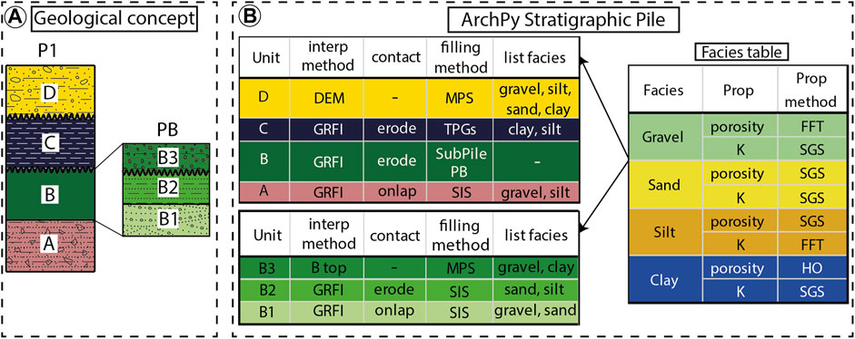
FIGURE 2. Schematic representation of an ArchPy stratigraphic pile (B) given a geological concept (A); interp. method, interpolation method; GRF, Gaussian random functions; DEM, digital elevation model; Prop method, property simulation method; MPS, multiple-points statistics; SIS, sequential indicator simulation; TPG, truncated pluri-Gaussians; HO, homogeneous; K, hydraulic conductivity; FFT, fast Fourier transform; SGS, sequential Gaussian simulation.

Thus, the stratigraphic pile is an object that can easily be manipulated and modified. Using such an approach, the user can focus more on the conceptual aspects of the modeling (unit relations, erosional events, spatial distribution of the lithologies or facies, etc.). In clear terms, the whole modeling process can be easily reproduced because all the steps are documented in the SP.

2.3 Erosion Rules

Erosion (stratigraphic) rules (ERs) describe how the surfaces influence each other after having been simulated. They are similar to those denominated “geological rules” by Calcagno et al. (2008). Figure 3 shows a simple example of the difference between onlap and erode behaviors. Here, two surfaces are simulated: S1 (old) and S2 (young), while the gray surface is simply set to the topography or the digital elevation model (DEM). S1 is defined onlap and S2 has both behaviors. If S2 is specified onlap, unit 2 (young, in black in the figure) is not deposited where S2 is below S1, whereas if S2 is specified erode, the effective top of unit 1 (young, in yellow in the figure) is set to S2. This approach allows incorporating geological time directly by choosing the appropriate truncation operation to remain consistent with the sedimentological history (Wellmann and Caumon, 2018). Another rule is that a surface cannot be above (or below) the DEM (resp. bottom of the domain); if this case arises, the surface will be automatically set to the DEM (resp. bottom). These ER are applied each time a new surface is simulated during the surface simulation.

FIGURE 3

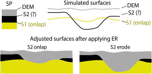
FIGURE 3. Schematic example of the erosion rules (ER) used in ArchPy. The surfaces are first simulated from oldest to youngest and then adjusted following the ER.

2.4 Synthetic Example

To illustrate the ArchPy capabilities, Figure 4 shows one stochastic realization of hydraulic conductivity and porosity based on the SP of Figure 2. The domain dimensions (x, y, z) are 3 × 1 × 0.2 km³ with a spatial resolution of 15 × 15 × 4 m³. The model is purely synthetic, but it mimics a valley filled by a series of sedimentary episodes. For this example, we assume that unit A is a moraine deposit only filled with gravel and silt. The B formation is deposited during three sub-steps (sub-pile PB, Figure 2). It represents a fluvio-glacial environment including three stages (B1, B2, and B3). On top of that, unit C is an important glacio-lacustrine phase where only fine particles are deposited (clay and silt). Unit D ends the process by setting up a fluvial environment that was more active in the southern part of the area (toward the -y main axis). The different steps to obtain this result will be explained in detail in the following sections.

FIGURE 4

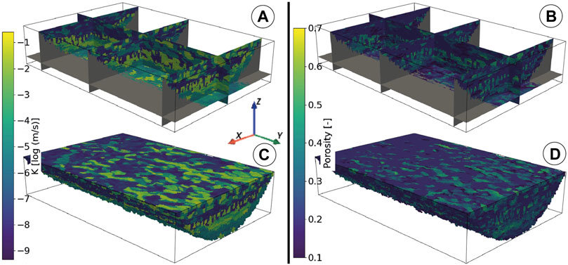
FIGURE 4. Realizations of two different properties ((A) hydraulic conductivity and (B) porosity) for the synthetic case. (C) and (D) are 3D blocs of the (A) and (B) realizations, respectively. The simulations used respective corresponding facies realizations of Figure 7 as simulation domains. Vertical exaggeration = 3x.

2.5 Data Pre-Processing

The main hard data to describe the geology in a Quaternary environment are the borehole information. For each borehole, ArchPy requires the following: a borehole ID, the depth, and location (x, y, and z) of the borehole as well as a stratigraphic unit log and/or a lithology log. Both logs contain the elevation of the top of the interpreted units and lithologies in the simulation grid reference system. These locations will be used as the conditioning point for simulations. An important thing to note is that the logs of borehole objects in the ArchPy interface only need top elevation for each unit/lithology encountered. To facilitate the geostatistical simulation of the properties, we consider only regular Cartesian grids for the moment in ArchPy (to avoid support effects). The extension and parameters of the grid are provided by the user. The SP and eventual sub-piles are also given as input. We then pre-process the borehole data (HD) to check that they are consistent with the SP and to extract the contact points between the units. The difficulty here (which is not intuitive) is that a contact between two units in a borehole does not necessarily correspond to the top of the unit located below this contact because of possible erosion or sedimentation hiatus. It is therefore necessary to analyze the borehole logs to identify the information that the contacts bring about the possible positions of the surfaces. To code this information, we will define contact points where the position of the surface is perfectly defined (equality contact point) and those which provide only indirect information (inequality contact point). Formally, an inequality contact point consists of a lower or upper bound for the actual surface.

Figure 5 shows how HD are interpreted automatically in the ArchPy pre-processing step given four different examples. We do not fully detail each example for brevity, but the main points are covered.

FIGURE 5

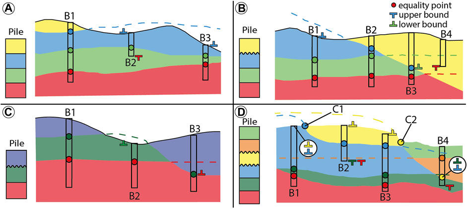
FIGURE 5. Four examples (A–D) of how inequalities and equalities are extracted from boreholes and field data. (B) indicates borehole information and (C) a unit contact (e.g., observed on the field). For each example, a stratigraphic pile is defined to indicate the relationships between the units and the nature of the surface contact (straight line is onlap and corrugated is erode). Dashed lines represent simulated surfaces before applying erosion rules (see Section 2.3).

Considering the example showed in Figure 5A, three surfaces need to be simulated: blue, green, and red tops (the yellow top is defined by the DEM). Equality points can be safely attributed in B1 between all contacts as there are no hiatus and no erosion layer in the Pile. However, in B2 and B3 boreholes, as the blue outcrops directly, its top must go above the surface, assuming erosion at the surface. This means that the tops of the borehole B2 and B3 are then lower bounds for the top of the blue unit. Also, the red unit is not encountered by B2 which indicates that it must go below the bottom of the borehole which is an upper bound for the top of the red unit. The Figure 5B example adds an erosional event (the blue top) that cross-cuts the green and red top layers. This implies that we must add an inequality contact point (lower bound) in B3 for the green top and equality contacts along the erosion surface (B2 and B3) for the blue top because of the ER. Indeed, the green top in B3 cannot be considered as the actual green top since the green unit has been eroded. The same event occurs in Figure 5C in B3 where the red unit has been eroded by an erosional event (the green top).

The more complex example (Figure 5D) shows that the number of extracted data can become important, especially when the number of layers increases. Here, additional outcrop information has been added with unit contacts (C1 and C2) that inform about a transition between two units. Yellow goes above as it is the unit reaching the topography. The contact between yellow and blue is an equality for blue (the only erode layer above blue is yellow, but it has been deposited and thus cannot have eroded blue). The bottom of B2 ends in the blue unit which indicates that all layers below it (dark green and red) must go below the bottom of the borehole. When two units in a borehole are separated by two (or more) erosion surfaces, ArchPy assumes that the contact belongs to the younger erosion surface. This is shown in Figure 5D at B4 between the orange and dark green units. In the pile, these two units are separated by two other units (blue and yellow) characterized by their erosional top. As yellow is younger than blue, the equality point is attributed to yellow.

All boreholes are then processed this way, and HD are extracted and assigned to respective surfaces. It is relevant to note that this step is completely automated in ArchPy and the only required inputs are the SP, the boreholes, and the simulation grid.

2.6 Simulation of the Surfaces and Units

Using the HD and the information provided by the SP, ArchPy performs a 2D simulation (interpolation) for each surface of the SP over the complete domain. Simulations are generally performed conditionally on HD, but unconditional simulations are also possible by defining a mean altitude.

The surfaces are simulated successively from the oldest to the most recent (for a hierarchic level). After having simulated a surface, we apply the ER (see Section 2.3). The surfaces are also simulated hierarchically, which implies that surfaces of higher order (main units) are simulated before those of lower order (subunits). For example, in the case of the pile in Figure 2, ArchPy first computes the surfaces of the top of A, B, and C, and only after, the surfaces of the top of B1 and B2 are computed inside the unit B. It means that no surface of the top of these subunits can go above or below the limits of B unit, even if it is an erode surface. The other lower hierarchical units (if present) are simulated following the same strategy. The top unit surface is not simulated since it must be equal to the digital elevation model (DEM) for consistency; it is then simply set as equal to the DEM. Equivalently, as lower limits of all units are defined by the top of the underlying unit, the bottom last unit must be defined. In ArchPy, this is done by setting it to the bottom of the simulation domain.

In the SP, the user must indicate an interpolation method for each layer among the following choices: simple and ordinary kriging (SK and OK, resp., Chilès and Delfiner, 2009), multi-Gaussian random functions with or without inequalities (GRF, Chilès and Delfiner, 2009), basic 2D interpolation methods (linear, nearest neighbors, and cubic) using SciPy (Virtanen et al., 2020), and, finally, direct sampling multiple-points statistics algorithm with or without inequalities (MPS, Mariethoz et al., 2010; Straubhaar and Renard, 2021). For the multi-Gaussian simulation methods, a normal-score transform can be applied automatically to the HD if they do not follow a Gaussian distribution. Most of the methods are taken from the Python module Geone that provides a set of geostatistical and MPS modeling tools. For each method, the user has to provide the set of required parameters. For example, for the kriging or multi-Gaussian simulations, a variogram model must be provided. The inference of the parameters can be done manually or automatically if sufficient data are available using the Geone toolbox. For the MPS approach, a training image and the relevant parameters also need to be provided. Anisotropy can be easily modeled by choosing appropriate variogram or MPS parameters.

Once all the surfaces of the SP are defined, it is straightforward to define the volumes representing the units (unit domains), knowing the top and bottom surfaces for each unit according to the ER. These volumes are discretized by defining which cells are intersected by the surfaces for each (x, y) location. All the cells lying vertically between these 2 cells are assigned to the unit domain. Concerning the intersected cells, they belong to the unit domain only if they go above (or below) the middle of the cell for the top surface (or bot resp.).

Figure 6 shows two realizations of the unit domains. The realizations are conditioned to the borehole data and the stratigraphic pile. The effect of using subunits is clearly visible: the B2 (middle green) top surface (which is set as erode) does not cross-cut unit A (as expected) in the front cross-section of both realizations. This approach allows for representing the uncertainty of the position and extension of the units. By running a large number of realizations, the uncertainty can be quantified: for example, probability maps can be produced for each unit by post-processing those results.

FIGURE 6

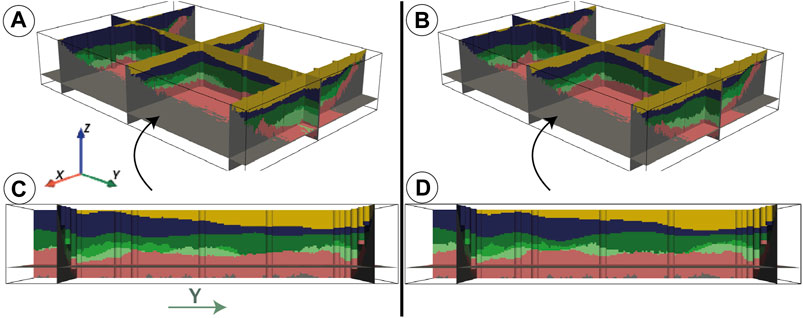
FIGURE 6. Two realizations (A,B) of the units (1st step of the ArchPy simulations) for the synthetic case. (C) and (D) are lateral view of the realizations (A) and (B), respectively. The colors of the units are those defined in the stratigraphic pile of Figure 2. They are presented with cross-sections for visualization purposes. Vertical exaggeration = 3x.

2.7 Simulation of the Facies

Once the stratigraphic unit volumes are defined, it is possible to fill these volumes with different facies or lithologies using different geostatistical methods. The simulation takes place in each unit independently, even if the same facies is present in different units, as in the example in Figure 2 where the sand appears in B and D units. This means that only the sand HD located inside the unit D will be taken into account when simulating the facies (sand) inside unit D. If a certain facies HD, which does not belong to a specific unit, is present inside its domain (e.g., a sand HD in unit C, Figure 2), these HD will be ignored. In such cases, warnings are issued by the software. This situation leads to inconsistencies with facies HD that principally reflect a probable mismatch in the HD (false geological interpretation) or in the geological concept.

As facies (resp. property) simulations are dependent on unit (resp. facies) simulation results, at least one facies (resp. property) simulation must be done for each unit (resp. facies) realization. It means that if the modeler chooses 100 unit realizations and 100 facies simulations, a total of 100 × 100 simulations will be generated. The same logic applies for the property simulations.

In the SP, the user must define one simulation method for each unit. The choices available in the current version of the code are as follows: homogeneous (one unique facies for the whole unit), sequential indicator simulations (SIS, Journel, 1983; Journel and Isaaks, 1984), Truncated pluri-Gaussians (TPG, Loc’h et al., 1994; Mariethoz et al., 2009; Armstrong et al., 2011), multiple-points statistics (MPS, Mariethoz et al., 2010; Straubhaar and Renard, 2021), and sub-pile which indicates that the unit will be populated by another pile containing subunits (e.g., PB in Figure 2).

Thus, multiple facies simulation techniques can be used to assess the uncertainty. Note that it is rather straightforward to switch from one method to another. This capability allows us to cover a broad uncertainty space by providing the user with different simulation methods within the same framework. Hence, if little geological knowledge is available for the spatial distribution of the facies within a unit, SIS can be used since little user inputs are required, while if there is more detailed geological knowledge available, other methods can be used, such as TPG or MPS, if an analog geological concept can be defined (e.g., training image). All the geostatistical methods used for this step are included inside Geone except for the TPG that are directly included inside ArchPy with various tools to define the truncated flag or estimate the variogram parameters of the underlying multi-Gaussian random fields.

Figure 7 shows two realizations of lithologies according to the unit realizations (Figure 6). The spatial variability of the lithologies is significant despite the fact that only four lithologies have been defined. This is mainly due to the combination of structural heterogeneity coming from the stratigraphic units and the lithology distribution within these units. This allows the exploration of many different plausible realities that are consistent with the HD and the concept. We can also observe the non-stationarity in unit D where the channels are sparser in the back than in the front (along the y axis). Indeed, it is important to mention that most of the facies simulation methods available in ArchPy can be non-stationary, allowing a much better representation of geological trends and exploration of the uncertainty.

FIGURE 7

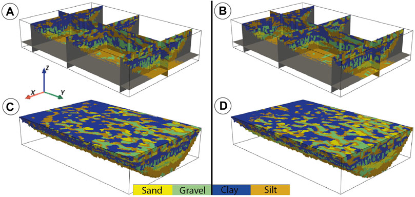
FIGURE 7. Two realizations (A,B) of the lithofacies (2nd step of the ArchPy simulations) for the synthetic case. (C,D) are 3D bloc realizations of (A) and (B), respectively. The simulations used the respective corresponding units of Figure 6 as simulation domains. Vertical exaggeration = 3x.

2.8 Simulation of the Properties

Once the facies are simulated, the simulation of the properties is straightforward and requires little input. Indeed, there are only two requirements: define the properties that must be simulated and define how to simulate them (method and parameters). The available methods for the moment are multi-Gaussian Random Fields (GRF) or homogeneous. If a GRF is used, two methods can be used to generate them: fast Fourier transform moving average (FFT, Ravalec et al., 2000) and sequential Gaussian simulation (SGS, Deutsch and Journel 1992). As the FFT method needs to perform the simulations on an entire grid, it can be less effective than SGS, especially if there are many lithologies and units. It is important to note that properties are simulated for a given lithofacies, independently and sequentially for each unit. For example, if we have a facies which is present in multiple units (consider the sand in Figure 2), the properties will be simulated first in the sand occurrences of the top unit and sequentially in the other occurrences in underlying units. This allows us to avoid spurious correlations that can arise if we consider the whole sand domains at once. Indeed, if sands of different units are in contact, they should not be considered as part of the same entity and thus should not be simulated together.

Conditional simulations are available with punctual data (x, y, z and property value). As some methods require at most one HD per cell, values that lie in the same cell are averaged if necessary.

2.9 Implementation of ArchPy

The ArchPy methodology is coded in an open-source Python code¹. The code is designed using an object-oriented approach. All the concepts described earlier are implemented using classes of objects designed to match the concepts and to facilitate their use. Most of the data imports and exports are based on simple text files. The geostatistical kernel of ArchPy is based on the Geone² Python library. For the visualization, ArchPy integrates some functionalities to produce various figures (e.g., stratigraphic units at a specific hierarchical level, only specified units, and cross-sections). These plots are generated mainly using PyVista³. If needed, data can also be exported in a vtk format for further use. Post-processing tools are also provided, to estimate, for example, the probability of encountering a specific unit (facies) or estimate the excepted value of a property over a part of the simulation domain. The structure and the principles underlying the ArchPy code are designed to allow the user to script the construction of the geological model in a very flexible manner. This also facilitates the coupling of ArchPy with any forward or inverse simulator. Some example Python notebooks are given on the online repository of the code.

3 A First Field Application

3.1 The Upper Aare Valley

The upper Aare Valley (Figure 8B) is a Quaternary alpine valley located between the cities of Thun and Bern in Switzerland with a complex and rich geological history due to its proximity to the Alps (Kellerhals et al., 1981; Haeuselmann et al., 2007). Previous studies on Quaternary deposits, on this particular site (Schlüchter, 1989; Preusser and Schlüchter, 2004) or at a regional scale (Preusser et al., 2011; Graf and Burkhalter, 2016), have shown the complex relations occurring between multiple depositional and erosional processes (mainly glacial, glacio-fluvial, and glacio-lacustrine). This led to the valley being incised and filled with a wide variety of sediments and facies (tills/moraines, fluvial gravels, glacio-lacustrine deposits, lake deposits, alluvial cones, etc.) explaining the great heterogeneity of this type of deposit. Two main aquifers have been identified in the valley: a superficial one which is actively used for drinking water supply, shallow geothermal energy, and some local industries and a deep one that is poorly known due to its higher depth (only few boreholes have reached it). Figure 8B shows that the superficial aquifer is mainly composed of the Aare gravels, the Late Glacial alluvial deposits, alluvial cones, and the Münsingen gravels.

FIGURE 8

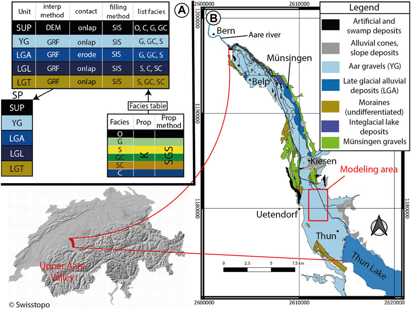
FIGURE 8. (A) Schematic stratigraphic pile used for the ArchPy simulations of the local geological models in the upper Aare Valley. It shows the different units that have been taken into account, their stratigraphic relations (which is above/below (i.e., younger/older)), the nature of its contact (erode or onlap), the interpolation methods used or the lithofacies (see Table 2), and the property to simulate (hydraulic conductivity (K) using sequential Gaussian simulations (SGS)). See Section 2.2 for more details. (B) Situation and simplified geological map of the upper Aare Valley. Only unconsolidated deposits that are near the aquifer are shown. The moraines are represented undifferentiated. The coordinates are presented in CH 1903+ - LV95 (epsg: 2056). All the data used come from the Swiss Geological Survey (Swisstopo).

A major hydrogeological synthesis of the valley was undertaken at the end of the 1970s and at the beginning of the 1980s (Kellerhals et al., 1981). Since then, additional data have been collected (Schlüchter (1989); Preusser and Schlüchter (2004)) for various projects in different parts of the valley, but no new hydrogeological synthesis has been assembled and published. Among the new data, the Swiss Geological Survey has systematically gathered the borehole data for Quaternary sediments in several pilot sites and homogenized the data and terminology (Volken et al., 2016). This data set includes around 800 digitized boreholes in the upper Aare Valley. A geological model of the valley filling has also been produced by the Swiss Geological Survey to illustrate how those data can be used. In addition, a valley scale towed Transient Electromagnetic Survey has been acquired and published in 2021 (Neven et al., 2021) by the University of Neuchâtel to better constrain and characterize the aquifer dimensions and its internal heterogeneity.

3.2 Modeling Area and Borehole Dataset

To illustrate the ArchPy approach, we chose an area with a high density of boreholes located in the south of the Valley (Figure 8B). The extent of this area is given by its coordinates in the CH 1903+ - LV95 system: lower left corner, 2′611′000 m/1′178′000 m, and upper-right corner, 2′613′000 m/1′182′000 m.

The depth of the boreholes rarely exceeds 50 m; they do not reach the deepest aquifer and stay in the shallow one that is 50–60 m thick in this part of the valley (Kellerhals et al., 1981). The data set contains a large part of the boreholes that have been drilled over decades in the area (Volken et al., 2016). Each borehole is described in terms of intervals with information about the granulometry (lithofacies), the units encountered, the quality of the interpretations, etc. However, unit data can be missing, contrary to granulometry data, meaning that for many boreholes, only lithofacies data are available. Granulometry information is described with one, two, or up to three different grain sizes, each defined with a USCS classification code (Casagrande, 1948). No hydraulic conductivity data have been taken into account.

The boreholes (133 in total) intercept a total of four major stratigraphic units: Aare young gravel (YG, Holocene), Late Glacial alluvial deposits (LGA, Holocene), late glacio-lacustrine deposits (LGL, Holocene), and Late Glacial Till (LGT, late Pleistocene). The LGT appears only on two boreholes on the southern part of this section of the aquifer and will therefore be difficult to model. YG and LGA are the most present units and constitute the largest part of the shallow aquifer in this area while LGL and LGT are more scattered and can be seen as its bottom.

Note that this stratigraphic pile is simplified given that 23 major stratigraphic units can be distinguished on the entire valley (Volken et al., 2016). However, most of these units are absent in the modeled area.

3.3 Modeling Settings

The extension of the simulation domain is 2 km in the W-E direction and 3.3 km in the N-S direction. The elevation ranges from 520 to 570 m a.s.l and the resolution is 15 × 15 × 1 m, which implies a number of cells of 134 × 220 × 60 (nx × ny × nz). The top of the domain is defined according to the DEM of Switzerland with a resolution of 25 × 25 m (DHM25, Swisstopo) and the bottom is defined by a raster map of the bedrock elevation (TopFels25, Swisstopo), also with a resolution of 25 × 25 m, both freely distributed by the Swiss Federal Office of Topography.

The units were defined mainly on the basis of the HD and the geological knowledge of this area (Kellerhals et al., 1981). Five units were recognized (Figure 8A). A superior unit (SUP) was added which includes superficial (soil and peat) and artificial (anthropogenic) deposits. No subunit has been defined as such data are not available in this actual dataset. The top surfaces of the units have been modeled with GRF to take the effect of inequalities into account, except for the SUP top surface which was set to the DEM as it is the most superficial unit. The associated covariance models (variograms) were estimated using an automatic fitting method (least squares optimization) on the HD. The optimized parameters are shown in Table 1. Most of the surfaces were defined as onlap except the LGA top surface which represents a former terrace of the Aare river, generally deposited at a slightly higher altitude than YG (Kellerhals et al., 1981).

TABLE 1

TABLE 1. Covariance model parameters (C: contribution and r: range) used for the surface interpolation of each surface. All models are isotropic, except the LGT one with an orientation of N-S for the major axis). No covariance model was fitted for SUP as its surface is defined by the DEM. Subscripts exp and sph indicate exponential and spherical covariance models.

In the HD, the lithofacies are described by up to three different grain sizes. We chose to only take the most present one for each layer and we also grouped certain similar USCS codes (Table 2) to reduce the number of lithofacies to 7: others (O), gravel (G), sand (S), clayey gravel (GC), clayey sand (SC), and clay (C). The other facies regroup superficial codes such as OH or Pt. Facies were then considered within a unit if their proportions exceed 5% (inside that specific unit).

TABLE 2

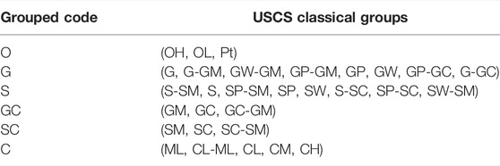
TABLE 2. Grouped USCS codes. It indicates in which group code the classical USCS groups are rearranged.

For the sake of simplicity in that example, all the units were filled using SIS. Prior variography analysis on the lithofacies HD shows significant variability which required the SIS variograms to be fitted manually; the chosen parameters are given in Table 3. Only the hydraulic conductivity K property has been simulated for that example using the covariance models given in Table 4. Note that adding other properties is possible and very simple since only the interpolation method and the covariance models (for each facies) are required.

TABLE 3

TABLE 3. Covariance model parameters (C: contribution and r: ranges in x, y, and z directions) manually adjusted and used for the SIS of each unit. For units where the number of data points was too low (LGL and LGT), a default model was taken (“Default” row). The ranges are given in the three main axis directions without any rotation (x axis goes toward E and y axis toward N). Subscripts exp and sph indicate exponential and spherical covariance models.

TABLE 4

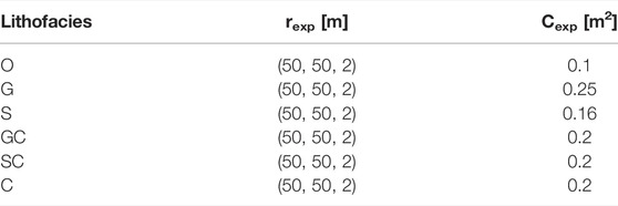
TABLE 4. Covariance model parameters (C: contribution and r: ranges in x, y, and z directions) used for the property simulations. Subscript exp indicates an exponential covariance model.

The ArchPy Aare model was run several times to illustrate its applicability for uncertainty estimation. In that example, we generated 10 simulations of the stratigraphic units. For each stratigraphic unit simulation, we generated 10 facies simulations. Finally, for each combined realization, we generated 1 unconditional simulation for K. This procedure resulted in a total of 100 simulations (10 × 10 × 1). The code allows us to proceed in this manner, but it also permits us to simulate all the components successively for each realization (units, facies, and properties). These different modes of simulation can be used for quantifying the impact of these different sources of uncertainty on the distribution of the properties but also on their groundwater flow or geophysical responses.

Figures 9–12 show the results of ArchPy simulations conditioned to the borehole data. The figures illustrate the type of heterogeneity and complexity that can be modeled rather simply using the ArchPy approach. For example, the two unit realizations (Figures 9A,B) differ significantly while being consistent and honoring both the borehole data. This variability is important for quantifying the uncertainty. To visualize that part of the uncertainty, ArchPy allows the user to compute the probability of observing a specific unit. Figure 10 shows in yellow the locations where it is quite certain that a given unit is present and with which thickness. For example, Figure 10A shows that the unit YG is well constrained in the eastern and northern part of the domain due to the important number of boreholes that reach it. The unit LGA seems to be more present in the southern part of the area (Figure 10B), thinner than the unit YG and almost absent (or very thin) in the north. The unit LGT (Figure 10C) does not display such trends and has a more uncertain distribution, probably mainly due to a lack of data (shallow boreholes).

FIGURE 9

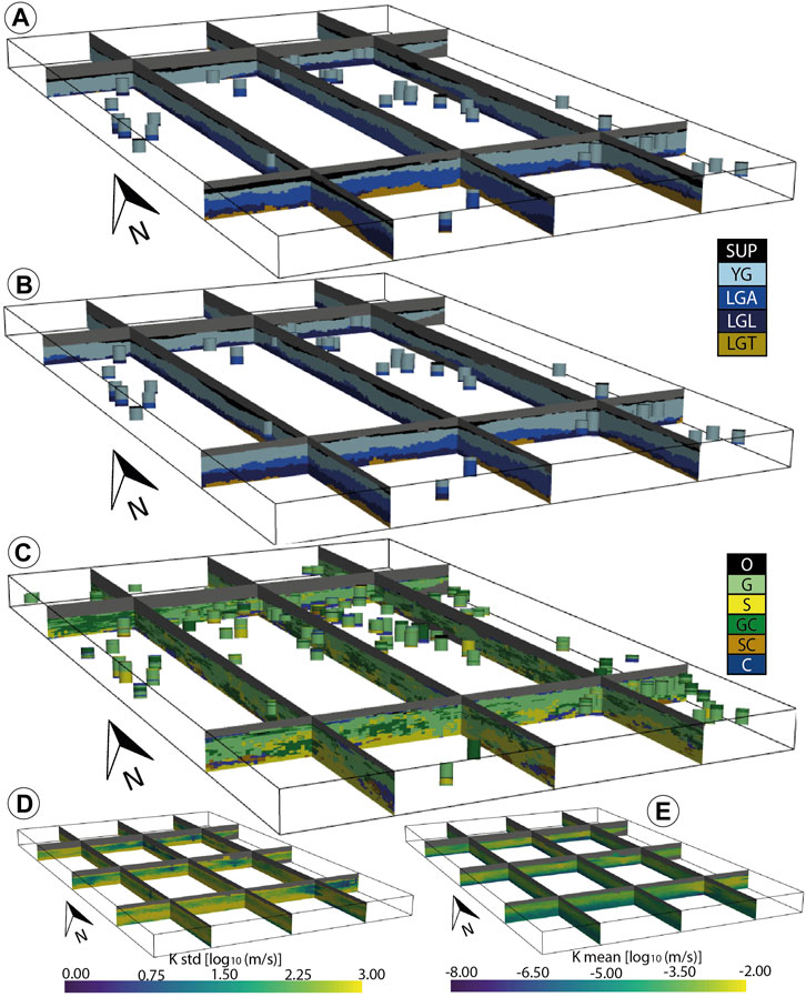
FIGURE 9. Aare aquifer results obtained for (A,B) two unit realizations, (C) one facies realization (within model (A)), and (D,E) K standard deviation and mean simulated along the 100 models; units are in log10 (m/s). Vertical exaggeration = 3x.

FIGURE 10

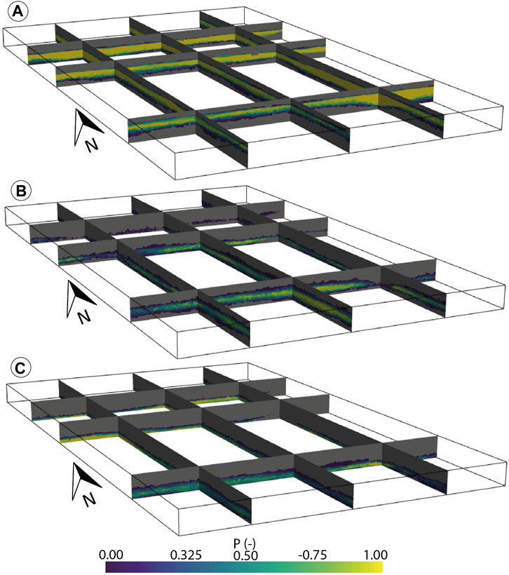
FIGURE 10. Probability of occurrence along the 100 models for units YG (A), LGA (B), and LGL (C). Vertical exaggeration = 3x.

Lithofacies simulations are shown in Figures 9C, 11 and are the results of the filling of the simulations shown in Figure 9A. These simulations honor both the borehole data and geometry of the stratigraphic units. As for the stratigraphic units, it is possible to compute and produce figures showing the probability of occurrence of each facies.

FIGURE 11

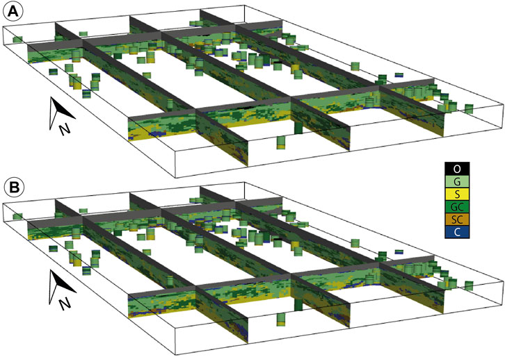
FIGURE 11. (A, B) Two facies realizations that are the results of the filling of the unit realization in Figure 9A. Boreholes show the spatial distribution of the HD.

Finally, two simulated hydraulic conductivity fields are shown in Figure 12. They display a broad range of values that is expected for this geology and that honor all the borehole data. It also shows the complex relations between the property values, the stratigraphic units, and the lithofacies. The variability between the realizations suggests a strong heterogeneity that would have been extremely difficult to model properly without the hierarchical approach (e.g., Feyen and Caers 2006; Zappa et al., 2006; Zech et al., 2021). The mean of the logarithm of K (Figure 9E) highlights the location of the aquifer where the values are likely to be especially high. These locations also coincide with those where the standard deviation (Figure 9D) is low, indicating that the property values are better defined inside the aquifer than outside. Elsewhere, the standard deviation values may be quite high, easily reaching 2 log₁₀ (m/s), indicating an uncertainty of up to two orders of magnitude. The variance is low around the boreholes as expected.

FIGURE 12

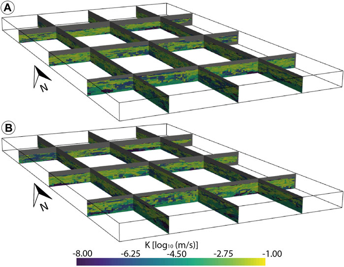
FIGURE 12. (A, B) Two property realizations made on the two facies realizations in Figure 11.

4 Discussion

One of the most important novel features of the ArchPy approach is the extended concept of stratigraphic pile (SP) as compared to the findings of Calcagno et al. (2008), for example. This concept has been shown to be an effective way to formulate all the geological knowledge into one entity (practically, a Python object). Thanks to this representation, it is easy to embed multiple SPs inside other SPs and to simulate the units to any level of hierarchy and do this without any particular restrictions. By including various interpolation and simulation methods which can be applied independently for each unit, lithofacies, and property, the ArchPy approach offers a high flexibility to the user who can adapt the methods to the quantity of available data and the complexity that he needs to represent for a specific site. In addition, the use of inequality data that are automatically derived from the SP and the borehole data allows ArchPy to extract a larger amount of information from boreholes than what is usually done in alternative geo-modeling tools.

The results obtained for the upper Aare Valley illustrate the type of stochastic models that can be easily and rapidly constructed for Quaternary deposits using the ArchPy approach. Due to the simple assumptions made about the geology and the concepts (simplified SP and use of SIS to fill the units), some aspects of the proposed method could not be illustrated in this example. Several limitations in the data set were also identified. For example, the LGT unit is not well constrained because only a few boreholes reach it. Indeed, most boreholes in this area are drilled for hydrogeological purposes (Kellerhals et al., 1981), and local communities are generally not interested in reaching the LGT unit because of its lower hydraulic conductivity as compared to the YG or LGA unit. A sampling bias is also expected in the lithofacies inside the LGL and LGT units. Indeed, we observe that the simulations of these units tend to have more sand (S code) than expected in glacio-lacustrine or till deposits. This can be due to a sampling bias in the borehole database because the areas of high permeability are preferentially drilled while clay and silt areas are generally avoided. Since the simulated proportions of lithofacies are conditioned on the HD, the lithofacies simulations can reflect this bias. It is, however, possible to correct it by imposing proportions that differ from those of the HD, but further secondary information should then be used to guide the simulations. One possible method to correct that bias could also be to use geophysical data, as we will discuss more in detail below.

Another important feature of the ArchPy approach is that it allows quantifying the uncertainty by generating an ensemble of models. The uncertainty can be evaluated at any desired hierarchical level among the units, subunits, sub-subunits, lithofacies, or properties. The uncertainty on the geological concept and stratigraphic pile (SP) itself can also be evaluated. This type of uncertainty was not covered in the example of the upper Aare valley, where the concept was simple. But there are situations in which different geological concepts or different geostatistical models for the different components of the SP are plausible. Using the ArchPy approach and its scripting possibilities, it is straightforward to automatically explore all these possibilities and generate an ensemble of models that covers this uncertainty.

Due to its recent existence, ArchPy still lacks some interesting features and has several limitations. First of all, it is only usable through scripts in Python, which may prevent a certain number of people from using it. However, examples are provided and can easily be edited; therefore, it is not necessary to be an expert in Python to use ArchPy. This approach has many advantages such as ensuring efficient model update when new data are acquired or accurately documenting the model construction steps. In future, one could construct a graphical user interface (GUI). The main limitation of ArchPy for the moment is that it assumes that the boundaries of the stratigraphic units can be modeled using functions that can be represented on a 2D grid. Therefore, ArchPy cannot, at the moment, represent overturned folds. It also does not include faults. We consider that these situations are extremely rare in Quaternary environments; adapting ArchPy to account for these structures would be feasible but is not currently a priority. ArchPy is also limited by the set of geostatistical methods that are proposed. It implies, for example, that the code may be slow if the number of borehole data and inequalities is important. We will continue to optimize the methods as much as possible. Concerning the simulation of non-Gaussian data, a normal-score transform should always be considered before using any GRF method. But the user must be aware that this kind of transformation is only suitable when the number of data is sufficient (a Cumulative Function Distribution can be built). When data are sparse, it is simply possible to assume that the data follow a normal distribution or the use of other available methods can be considered (MPS). Moreover, GRF simulations, performed on data normally transformed, do not guarantee that the covariance will be preserved in the original data space. The use of more advanced simulation methods such as Direct Sequential Simulation (Soares, 2001) could be a solution. The final note is about the trends in the data (surface elevations or facies proportions). Such behaviors can be modeled but not in a fully automated manner as it requires user-inputs (e.g., local facies proportions over the domain). These must be computed or derived externally. However, implementing such routines in future updates is straightforward.

Because it is simple and easy to run ArchPy automatically, it is straightforward to conduct parameter sensitivity analysis. We even suggest that the parameters should be tested as well as the stratigraphic pile, including all its various geostatistical components, using cross-validation. This approach should be used to test and compare different alternative SPs. The procedure consists in splitting the borehole data and applying a K-fold cross-validation approach as we discussed in a previous study (Juda et al., 2020). An ensemble of models is generated to predict the units, lithologies, and properties at the location of a subset of the boreholes (removed from the HD). A score can then be computed to compare the quality of the stochastic predictions with the actual data. We plan to incorporate cross-validation frameworks inside the ArchPy architecture.

To go a step further, ArchPy is already coupled with several geophysical and groundwater flow simulation tools Cockett et al. (2015); Bakker et al. (2016). Property models generated using ArchPy (e.g., resistivity, gravity, storativity, and hydraulic conductivity) can be passed to forward models. The outputs are retrieved and compared with real field measurements which are then used to adapt the ArchPy models to reduce the misfit between both actual and simulated data. For example, this adaptation could be done in a Monte Carlo scheme (Tokdar and Kass 2010) or with ensemble methods (Chen and Oliver, 2012). This approach opens the way toward geologically constrained joint inversion involving different forward models.

5 Conclusion

The ArchPy approach that is proposed in this study combines many techniques that are well known (geostatistical simulation techniques for continuous or categorical variables). One important novelty is to formally separate the description of the list of tasks that are required to construct the model and the construction of the model itself. This is done by embedding all the geological and geostatistical knowledge in an object called “stratigraphic pile.” Based on this formalism, a piece of software can be constructed that can automate all the tedious tasks of the model construction. The Python module that implements the ArchPy approach allows the fast and reproducible creation of an ensemble of stochastic models respecting both the conditional data and the user inputs (geological concepts). The only inputs required are the digital elevation model, the borehole data, and how to interpolate and simulate the different components of the model (surfaces, lithofacies, and properties); the rest is up to ArchPy. The simulations take place during three main phases: simulation of the units, of the lithofacies, and then of the properties. Each step depends on the previous ones. A major novelty is that the stratigraphic pile allows defining a hierarchical stratigraphy and therefore allows modeling automatically consistent subunits of any hierarchical level within units of higher levels. The code allows quantifying uncertainty using a sound geostatistical model. It also allows updating the model easily when new data are available or embedding the model construction into an inverse procedure. The code is open-source and freely distributed. Due to its open-source nature, the coupling with other software is facilitated. It opens the doors to an easier and more accessible geological modeling of Quaternary aquifers.

Data Availability Statement

The github repository of the code as well as the synthetical dataset used can be found on http://www.github.com/randlab/ArchPy. The data concerning the Aar model are available on request at the Swiss geological survey, Swisstopo.

Author Contributions

LS: ArchPy software development and data preparation. JS: Geone library development and support. LS and PR: conceptualization and methodology. LS: original draft preparation and editing. PR and JS: review and editing. PR: funding acquisition, supervision, and project administration. All authors contributed to the article and approved the submitted version.

Funding

This research is funded by the Swiss National Science Foundation under the contract 200020_182600/1 (PheniX project).

Conflict of Interest

The authors declare that the research was conducted in the absence of any commercial or financial relationships that could be construed as a potential conflict of interest.

Publisher’s Note

All claims expressed in this article are solely those of the authors and do not necessarily represent those of their affiliated organizations, or those of the publisher, the editors, and the reviewers. Any product that may be evaluated in this article, or claim that may be made by its manufacturer, is not guaranteed or endorsed by the publisher.

Acknowledgments

The authors would like to greatly thank Alexis Neven for the discussions about the design of ArchPy, his active use of the code, and, thus, for his help in finding most of the bugs and issues. The authors also thank all the partners of the project for their inputs and discussions and, in particular, the Swiss Geological Survey (Swisstopo) for having prepared and shared the dataset, the Canton of Bern, and GEOTEST AG as well as KELLERHALS + HAEFELI AG for their support. The authors would also like to thank two reviewers who helped to improve the quality of this article.

Footnotes

¹http://www.github.com/randlab/ArchPy.

²http://www.github.com/randlab/geone.

³https://www.pyvista.org/.

References

Aigner, T., Asprion, U., Hornung, J., Junghans, W.-D., and Kostrewa, R. (1996). Integrated Outcrop Analogue Studies for Triassic Alluvial Reservoirs: Examples from Southern germany. J. Pet. Geol. 19, 393–406. doi:10.1111/j.1747-5457.1996.tb00446.x

CrossRef Full Text | Google Scholar

Armstrong, M., Galli, A., Beucher, H., Loc’h, G., Renard, D., Doligez, B., et al. (2011). Plurigaussian Simulations in Geosciences. Springer Science & Business Media.

Google Scholar

Bakker, M., Post, V., Langevin, C. D., Hughes, J. D., White, J. T., Starn, J. J., et al. (2016). Scripting Modflow Model Development Using python and Flopy. Groundwater 54, 733–739. doi:10.1111/gwat.12413

PubMed Abstract | CrossRef Full Text | Google Scholar

Bennett, J. P., Haslauer, C. P., Ross, M., and Cirpka, O. A. (2019). An Open, Object‐Based Framework for Generating Anisotropy in Sedimentary Subsurface Models. Groundwater 57, 420–429. doi:10.1111/gwat.12803

PubMed Abstract | CrossRef Full Text | Google Scholar

Biegler, L., Biros, G., Ghattas, O., Heinkenschloss, M., Keyes, D., Mallick, B., et al. (2011). Large-Scale Inverse Problems and Quantification of Uncertainty. John Wiley & Sons.

Google Scholar

Bridge, J. S. (2009). Rivers and Floodplains: Forms, Processes, and Sedimentary Record. John Wiley & Sons.

Google Scholar

Calcagno, P., Chilès, J. P., Courrioux, G., and Guillen, A. (2008). Geological Modelling from Field Data and Geological Knowledge. Phys. Earth Planet. Interiors 171, 147–157. doi:10.1016/j.pepi.2008.06.013

CrossRef Full Text | Google Scholar

Casagrande, A. (1948). Classification and Identification of Soils. T. Am. Soc. Civ. Eng. 113, 901–930. doi:10.1061/TACEAT.0006109

CrossRef Full Text | Google Scholar

Chen, Y., and Oliver, D. S. (2012). Ensemble Randomized Maximum Likelihood Method as an Iterative Ensemble Smoother. Math. Geosci. 44, 1–26. doi:10.1007/s11004-011-9376-z

CrossRef Full Text | Google Scholar

Chilès, J.-P., and Delfiner, P. (2009). Geostatistics: Modeling Spatial Uncertainty. John Wiley & Sons.

Google Scholar

Cockett, R., Kang, S., Heagy, L. J., Pidlisecky, A., and Oldenburg, D. W. (2015). Simpeg: An Open Source Framework for Simulation and Gradient Based Parameter Estimation in Geophysical Applications. Comput. Geosciences 84, 142–154. doi:10.1016/j.cageo.2015.09.015

CrossRef Full Text | Google Scholar

Comunian, A., De Micheli, L., Lazzati, C., Felletti, F., Giacobbo, F., Giudici, M., et al. (2016). Hierarchical Simulation of Aquifer Heterogeneity: Implications of Different Simulation Settings on Solute-Transport Modeling. Hydrogeol. J. 24, 319–334. doi:10.1007/s10040-015-1343-1

CrossRef Full Text | Google Scholar

Comunian, A., Renard, P., Straubhaar, J., and Bayer, P. (2011). Three-dimensional High Resolution Fluvio-Glacial Aquifer Analog - Part 2: Geostatistical Modeling. J. Hydrology 405, 10–23. doi:10.1016/j.jhydrol.2011.03.037

CrossRef Full Text | Google Scholar

de la Varga, M., Schaaf, A., and Wellmann, F. (2019). GemPy 1.0: Open-Source Stochastic Geological Modeling and Inversion. Geosci. Model Dev. 12, 1–32. doi:10.5194/gmd-12-1-2019

CrossRef Full Text | Google Scholar

Deutsch, C. V., and Journel, A. G. (1992). GSLIB. Geostatistical Software Library and User’s Guide. New York: Oxford University Press.

Google Scholar

Dubrule, O., and Kostov, C. (1986). An Interpolation Method Taking into Account Inequality Constraints: I. Methodology. Math. Geol. 18, 33–51. doi:10.1007/BF00897654

CrossRef Full Text | Google Scholar

Feyen, L., and Caers, J. (2006). Quantifying Geological Uncertainty for Flow and Transport Modeling in Multi-Modal Heterogeneous Formations. Adv. Water Resour. 29, 912–929. doi:10.1016/j.advwatres.2005.08.002

CrossRef Full Text | Google Scholar

Ford, G. L., and Pyles, D. R. (2014). A Hierarchical Approach for Evaluating Fluvial Systems: Architectural Analysis and Sequential Evolution of the High Net-Sand Content, Middle Wasatch Formation, Uinta Basin, Utah. Bulletin 98, 1273–1303. doi:10.1306/12171313052

CrossRef Full Text | Google Scholar

Freulon, X., and de Fouquet, C. (1993). “Conditioning a Gaussian Model with Inequalities,” in Geostatistics Tróia ’92. Editor A. Soares (Dordrecht: Springer Netherlands), Quantitative Geology and Geostatistics), 1, 201–212. doi:10.1007/978-94-011-1739-5_17

CrossRef Full Text | Google Scholar

Graf, H. R., and Burkhalter, R. (2016). Quaternary Deposits: Concept for a Stratigraphic Classification and Nomenclature-An Example from Northern Switzerland. Swiss J. Geosci. 109, 137–147. doi:10.1007/s00015-016-0222-7

CrossRef Full Text | Google Scholar

Haeuselmann, P., Granger, D. E., Jeannin, P.-Y., and Lauritzen, S.-E. (2007). Abrupt Glacial Valley Incision at 0.8 Ma Dated from Cave Deposits in Switzerland. Geol 35, 143–146. doi:10.1130/G23094A

CrossRef Full Text | Google Scholar

Heinz, J. r., and Aigner, T. (2003). Hierarchical Dynamic Stratigraphy in Various Quaternary Gravel Deposits, Rhine Glacier Area (SW Germany): Implications for Hydrostratigraphy. Int. J. Earth Sci. 92, 923–938. doi:10.1007/s00531-003-0359-2

CrossRef Full Text | Google Scholar

Journel, A. G., and Isaaks, E. H. (1984). Conditional Indicator Simulation: Application to a Saskatchewan Uranium Deposit. Math. Geol. 16, 685–718. doi:10.1007/BF01033030

CrossRef Full Text | Google Scholar

Journel, A. G. (1983). Nonparametric Estimation of Spatial Distributions. Math. Geol. 15, 445–468. doi:10.1007/BF01031292

CrossRef Full Text | Google Scholar

Juda, P., Renard, P., and Straubhaar, J. (2020). A Framework for the Cross‐Validation of Categorical Geostatistical Simulations. Earth Space Sci. 7, e2020EA001152. doi:10.1029/2020EA001152

CrossRef Full Text | Google Scholar

Kellerhals, P., Haefeli, C., and Tröhler, B. (1981). Grundlagen für Schutz und Bewirtschaftung der Grundwasser des Kantons Bern Hydrogeologie Aaretal, zwischen Thun und Bern. Tech. rep. Bern: Wasser- u. Energiewirtschaftsamt des Kantons Bern.

Google Scholar

Koltermann, C. E., and Gorelick, S. M. (1996). Heterogeneity in Sedimentary Deposits: A Review of Structure-Imitating, Process-Imitating, and Descriptive Approaches. Water Resour. Res. 32, 2617–2658. doi:10.1029/96wr00025

CrossRef Full Text | Google Scholar

Le Loc’h, G., Beucher, H., Galli, A., and Doligez, B. (1994). Improvement in the Truncated Gaussian Method: Combining Several Gaussian Functions. ECMOR IV - 4th European Conference on the Mathematics of Oil Recovery, Roros, Norway. European Association of Geoscientists & Engineers. doi:10.3997/2214-4609.201411149

CrossRef Full Text | Google Scholar

Mallet, J.-L. (1989). Discrete Smooth Interpolation. ACM Trans. Graph. 8, 121–144. doi:10.1145/62054.62057

CrossRef Full Text | Google Scholar

Mariethoz, G., Renard, P., Cornaton, F., and Jaquet, O. (2009). Truncated Plurigaussian Simulations to Characterize Aquifer Heterogeneity. Groundwater 47, 13–24. doi:10.1111/j.1745-6584.2008.00489.x

PubMed Abstract | CrossRef Full Text | Google Scholar

Mariethoz, G., Renard, P., and Straubhaar, J. (2010). The Direct Sampling Method to Perform Multiple-point Geostatistical Simulations. Water Resour. Res. 46. doi:10.1029/2008WR007621

CrossRef Full Text | Google Scholar

Matheron, G. (1963). Principles of Geostatistics. Econ. Geol. 58, 1246–1266. doi:10.2113/gsecongeo.58.8.1246

CrossRef Full Text | Google Scholar

Miall, A. (1991). “Hierarchies of Architectural Units in Terrigenous Clastic Rocks and Their Relationship to Sedimentation Rate,” in The Three-Dimensional Facies Architecture of Terrigenous Clastic Sediments, and its Implications for Hydrocarbon Discovery and Recovery. Editors A. D. Miall, and N. Tyler (tulsa, oklahoma: Society for sedimentary geology edn), 3. doi:10.2110/csp.91.03.0006

CrossRef Full Text | Google Scholar

Neuman, S. P. (1990). Universal Scaling of Hydraulic Conductivities and Dispersivities in Geologic Media. Water Resour. Res. 26, 1749–1758. doi:10.1029/wr026i008p01749

CrossRef Full Text | Google Scholar

Neven, A., Maurya, P. K., Christiansen, A. V., and Renard, P. (2021). tTEM20AAR: A Benchmark Geophysical Data Set for Unconsolidated Fluvioglacial Sediments. Earth Syst. Sci. Data 13, 2743–2752. doi:10.5194/essd-13-2743-2021

CrossRef Full Text | Google Scholar

Preusser, F., Graf, H. R., Keller, O., Krayss, E., and Schlüchter, C. (2011). Quaternary Glaciation History of Northern Switzerland. E&G Quat. Sci. J. 60, 282–305. doi:10.3285/eg.60.2-3.06

CrossRef Full Text | Google Scholar

Preusser, F., and Schlüchter, C. (2004). Dates from an Important Early Late Pleistocene Ice Advance in the Aare Valley, Switzerland. Eclogae Geol. Helv. 97, 245–253. doi:10.1007/s00015-004-1119-4

CrossRef Full Text | Google Scholar

Pyrcz, M. J., and Deutsch, C. V. (2014). Geostatistical Reservoir Modeling. Oxford University Press.

Google Scholar

Ramanathan, R., Guin, A., Ritzi, R. W., Dominic, D. F., Freedman, V. L., Scheibe, T. D., et al. (2010). Simulating the Heterogeneity in Braided Channel Belt Deposits: 1. A Geometric-Based Methodology and Code. Water Resour. Res. 46. doi:10.1029/2009wr008111

CrossRef Full Text | Google Scholar

Ravalec, M. L., Noetinger, B., and Hu, L. Y. (2000). The FFT Moving Average (FFT-MA) Generator: An Efficient Numerical Method for Generating and Conditioning Gaussian Simulations. Math. Geol. 32, 701–723. doi:10.1023/a:1007542406333

CrossRef Full Text | Google Scholar

Renard, P., and Courrioux, G. (1994). Three-dimensional Geometric Modeling of a Faulted Domain: The Soultz Horst Example (Alsace, france). Comput. Geosciences 20, 1379–1390. doi:10.1016/0098-3004(94)90061-2

CrossRef Full Text | Google Scholar

Ringrose, P., and Bentley, M. (2016). Reservoir Model Design. Springer.

Google Scholar

Ritzi, R. W., Dai, Z., Dominic, D. F., and Rubin, Y. N. (2004). Spatial Correlation of Permeability in Cross-Stratified Sediment with Hierarchical Architecture. Water Resour. Res. 40. doi:10.1029/2003wr002420

CrossRef Full Text | Google Scholar

Scheibe, T. D., and Freyberg, D. L. (1995). Use of Sedimentological Information for Geometric Simulation of Natural Porous Media Structure. Water Resour. Res. 31, 3259–3270. doi:10.1029/95wr02570

CrossRef Full Text | Google Scholar

Schlüchter, C. (1989). The Most Complete Quaternary Record of the Swiss Alpine Foreland. Palaeogeogr. Palaeoclimatol. Palaeoecol. 72, 141–146. doi:10.1016/0031-0182(89)90138-7

CrossRef Full Text | Google Scholar

Soares, A. (2001). Direct Sequential Simulation and Cosimulation. Math. Geol. 33, 911–926. doi:10.1023/a:1012246006212

CrossRef Full Text | Google Scholar

Straubhaar, J., and Renard, P. (2021). Conditioning Multiple-Point Statistics Simulation to Inequality Data. Earth Space Sci. 8, e2020EA001515. doi:10.1029/2020EA001515

CrossRef Full Text | Google Scholar

Tokdar, S. T., and Kass, R. E. (2010). Importance Sampling: A Review. WIREs Comp. Stat. 2, 54–60. doi:10.1002/wics.56

CrossRef Full Text | Google Scholar

Virtanen, P., Gommers, R., Oliphant, T. E., Haberland, M., Reddy, T., Cournapeau, D., et al. (2020). SciPy 1.0: Fundamental Algorithms for Scientific Computing in Python. Nat. Methods 17, 261–272. doi:10.1038/s41592-019-0686-2

PubMed Abstract | CrossRef Full Text | Google Scholar

Volken, S., Preisig, G., and Gaehwiler, M. (2016). GeoQuat: Developing a System for the Sustainable Management, 3D Modelling and Application of Quaternary Deposit Data. Swiss Bull. Appl. Geol. 21, 3–16.

Google Scholar

Weissmann, G. S., and Fogg, G. E. (1999). Multi-scale Alluvial Fan Heterogeneity Modeled with Transition Probability Geostatistics in a Sequence Stratigraphic Framework. J. Hydrology 226, 48–65. doi:10.1016/s0022-1694(99)00160-2

CrossRef Full Text | Google Scholar

Wellmann, F., and Caumon, G. (2018). 3-D Structural Geological Models: Concepts, Methods, and Uncertainties. Adv. Geophys. 59, 1–121. doi:10.1016/bs.agph.2018.09.001

CrossRef Full Text | Google Scholar

Zappa, G., Bersezio, R., Felletti, F., and Giudici, M. (2006). Modeling Heterogeneity of Gravel-Sand, Braided Stream, Alluvial Aquifers at the Facies Scale. J. Hydrology 325, 134–153. doi:10.1016/j.jhydrol.2005.10.016

CrossRef Full Text | Google Scholar

Zech, A., Dietrich, P., Attinger, S., and Teutsch, G. (2021). A Field Evidence Model: How to Predict Transport in Heterogeneous Aquifers at Low Investigation Level. Hydrol. Earth Syst. Sci. 25, 1–15. doi:10.5194/hess-25-1-2021

CrossRef Full Text | Google Scholar

Zuffetti, C., Comunian, A., Bersezio, R., and Renard, P. (2020). A New Perspective to Model Subsurface Stratigraphy in Alluvial Hydrogeological Basins, Introducing Geological Hierarchy and Relative Chronology. Comput. Geosciences 140, 104506. doi:10.1016/j.cageo.2020.104506

CrossRef Full Text | Google Scholar