Characterization of Pyrolysis Kinetics of Continental Shale: Comparison and Enlightenment of the Parallel Reaction Model and the Overall Reaction Model

A total of nine immature–low maturity oil shale samples from Fushun and Maoming, the main oil shale producing areas in China, and three mature shale samples from the Jiyang Depression, China, were selected for use in hydrocarbon generation thermal simulation experiments in an open system and a closed system. The parallel first–order reaction kinetic model and the overall nth–order reaction kinetic model were used to calibrate the pyrolysis kinetic parameters of the samples. This comparative study revealed following conclusion. The generation period of the gaseous hydrocarbons (C_1–5) was the longest, and the generation period of the heavy hydrocarbon (C₁₄₊) was the shortest. The activation energy of the hydrocarbon generation reaction was closely related to the maturity of the organic matter, i.e., the higher the maturity of the sample, the higher the activation energy of the reaction, which indicates that oil shale/shale oil conversion requires higher temperature conditions. The parallel first–order reaction model regards the hydrocarbon generation reaction as a series of first–order reactions, and it has a better fitting effect for the longer hydrocarbon generation period reactions, such as generating gaseous hydrocarbons (C_1–5) and light components (C_6–14) from organic matter. The overall nth–order reaction treats the reaction as a nth–order reaction, and the nth–order reaction has a better fitting effect for reactions with a narrow hydrocarbon generation window, such as generating heavy components from organic matter. In the process of generating hydrocarbons from organic matter, the order of the reaction is the sum of the orders of the sub–reactions. The more hydrocarbon–generating parent material, the higher order of hydrocarbon–generating reaction. The reaction order sequence of the generation of different hydrocarbons from organic matter is as follows: generation of gaseous hydrocarbons > generation of light hydrocarbons > generation of heavy hydrocarbons.

1 Introduction

The nature of the conversion of organic matter into oil and natural gas under geological conditions is a chemical reaction process with a long reaction time, which can be quantitatively characterized by chemical kinetic methods (Braun and Burnham, 1987; Burnham and Sweeney, 1989; Pepper and Corvi, 1995; Burnham and Braun, 1999; Dieckmann, 2005). First, thermal simulation data are used to establish a chemical kinetic model of hydrocarbon generation from organic matter (Behar et al., 1997; Chen et al., 2017a). Then, it is extrapolated to geological conditions for application in the kinetic simulation of hydrocarbon generation from organic matter during geological periods, reconstructing the hydrocarbon generation history (Wang et al., 2013; Han et al., 2014; Chen et al., 2017b; Chen et al., 2017c; Li et al., 2018; Chen et al., 2020; Johnson et al., 2020; Wang et al., 2020). Hydrocarbon generation kinetics models are also applicable to product prediction in the in situ conversion of oil shale (Kang et al., 2020; He et al., 2021; Zhang et al., 2021) and low–maturity shale oil (Zhang et al., 2019).

Kinetic models include the overall reaction model (Allred, 1966; Haddadin and Tawarah, 1980; Shih and Sohn, 1980), the Friedman type model (Klomp and Wright, 1990), the sequential reaction model (Behar et al., 2008), and the parallel reaction model (Tissot et al., 1987; Ritter et al., 1993; Burnham et al., 1995). Due to the large amount of calculations required to calibrate these models and the limited data processing capability of early computers, researchers initially used the overall reaction model. The Friedman type model is essentially a piecewise overall reaction model. The sequential reaction model obtains the final product through several consecutive elementary reactions, and the product of the previous elementary reaction is the reactant of the last reaction. However, this model has high experimental requirements and had not been applied in large–scale. The parallel reaction model regards hydrocarbon generation from kerogen as finite number of parallel reactions, and is the most widely used kinetic model at present.

To simplify the model, the parallel reaction kinetic model assume that each parallel reaction is a first–order reaction, which means that the reaction rate is only proportional to the first power of the concentration of the reacting substance. The parallel first–order reaction kinetic model uses the quantity and distribution characteristics of the parallel reactions to characterize the reaction process. The overall nth–order reaction model treats the reaction as a whole reaction, but the order of the reaction is not limited to first order. The order of the reaction refers to the algebraic sum of the exponents of the substance concentration terms in the power series rate equation of a chemical reaction, which is usually represented by n. If the power series rate equation of the reaction is $v=k{C}_A^a{C}_B^b{C}_C^c\mathrm{...}$, then the order of the reaction is $n=a+b+c\mathrm{...}$. Generally speaking, the order of the reaction is that of the total reaction. a, b, and c are the orders of the reactions of reactants A, B, and C, respectively, which means that the order of the reaction is a for A, b for B, c for C, and so on. The reaction order reflects the degree of influence of the substance’s concentration on the reaction rate. The larger the order of the reaction, the more the reaction rate is affected by the concentration.

The parallel first–order reaction model assumes that the process of hydrocarbon generation from kerogen consists of a series of parallel first–order reactions (N); each reaction has its own activation energy (E_i) and frequency factor (A_i), and for each reaction, the corresponding original hydrocarbon generation potential of the kerogen is X_i0, i = 1, 2, 3, … N. When a certain reaction time t is reached, the hydrocarbon generation potential of the ith reaction is X_i, as shown in Eq 1 (Burnham et al., 1995).

$\begin{array}{l}\frac{d\left(X_i\right)}{d\left(t\right)}=K_i\left(X_{i0}-X_i\right)\\ i=\mathrm{1,2},\mathrm{...},N\end{array}(1)$

K_i is the reaction rate constant of the ith kerogen hydrocarbon generation reaction, which can be obtained using the Arrhenius formula as follows:

$\begin{array}{l}{K}_i=A_i\exp \left(\frac{-E_i}{RT}\right)\\ i=\mathrm{1,2},\mathrm{...},N\end{array}(2)$

Because the organic matter pyrolysis experiments under laboratory conditions involved constant heating (assuming the heating rate is D), then

$\frac{d\left(T\right)}{d\left(t\right)}=D(3)$

By combining the above formulas, it was determined that the amount of hydrocarbon generation during the ith reaction is

$X_i=X_{i0}\left(1-\exp \left(-{\displaystyle {\int }_{T_0}^T\frac{A_i}{D}}\cdot \exp \left(-\frac{E_i}{RT}\right)dT\right)\right)(4)$

The total hydrocarbon production of all of the parallel reactions is

$X={\displaystyle \sum _{i=1}^N{X}_i={\displaystyle \sum _{i=1}^N\left(X_{i0}\left(1-\exp -{\displaystyle {\int }_{T_0}^T\frac{A_i}{D}\cdot \exp \left(-\frac{E_i}{RT}\right)DT}\right)\right)}}(5)$

Similarly, Overall first order reaction and overall nth–order reaction models are as shown in Eqs. 6, 7, respectively (Allred, 1966). In the past, researchers usually used the plotting method to calibrate the kinetic parameters of overall reaction. Based on the transformation of kinetic equation, the linear relationship between kinetic parameters and experimental data was established, and the kinetic parameters were continuously adjusted manually to optimize the linear relationship (Haddadin and Tawarah, 1980; Shih and Sohn, 1980). Therefore, the calculation efficiency of the plotting method is low and the error is large.

$X=1-\exp \left(-{\displaystyle {\int }_{T0}^T\frac{A}{D}\exp \left(-\frac{E}{RT}\right)}dT\right)\left(n=1\right)(6)$

$X=1-{\left(1-\left(1-n\right){\displaystyle {\int }_{T0}^T\frac{A}{D}\exp \left(-\frac{E}{RT}\right)}dT\right)}^{\frac{1}{1-n}}\left(n\ne 1\right)(7)$

Theoretically, the parallel first–order reaction model is more reasonable than the overall first–order reaction model, and the overall non first–order reaction model is more reasonable in setting the reaction order, but there is still a lack of comparative research between the two types of models. In this study, the pyrolysis hydrocarbon generation characteristics were studied through the pyrolysis experiments of open and closed systems, and the kinetic characteristics of samples were characterized by parallel first–order reaction model and general package multistage non first–order reaction kinetic model, in order to deepen the understanding of the applicability of the model and the reaction mechanism of hydrocarbon generation of organic matter.

2 Samples and Experiments

2.1 Samples

Six oil shale samples from burial depths of 120–140 m in the Maoming oil shale production area in Guangdong, China, and three oil shale samples from burial depths of 400–450 m in the Fushun oil shale production area in Liaoning, China, were selected for the experiments. In addition, three mature shale samples from a buried depth of about 3,000 m in the Jiyang Depression, China, were selected for comparison to study the influence of the organic matter’s maturity on the kinetic characteristics.

2.2 Experiments

Routine rock pyrolysis and total organic carbon (TOC) detection were performed on the selected samples to obtain their basic geochemical parameters, such as the TOC, organic matter maturity, and type of organic matter (Hazra and Dutta, 2017; Chen et al., 2021). Then, the thermal simulation was carried out, which included Rock–Eval, pyrolysis–gas chromatography (PY–GC) in an open system, and thermal simulation experiments of gold tube in a closed system.

2.2.1 TOC Measurement

The TOC analysis was performed using a LECO CS–230HC analyzer. Approximately 250–500 mg of 100–120 mesh rock was required. To remove the inorganic carbon in the form of carbonates, it was necessary to acidify the sample before analysis. The samples were rinsed with distilled water to remove the HCl solution. After this, the samples were dried to eliminate moisture prior to analysis. The prepared sample was placed in the oven of the analyzer and heated at 1,100 °C, and the amount of carbon dioxide (CO₂) produced was measured using an infrared cell. The samples were subjected to quality assurance/quality control (QA/QC) analysis in duplicate to ensure that the analysis accuracy is better than ±0.2%.

2.2.2 Rock–Eval Pyrolysis

A Rock–Eval–VI pyrolysis apparatus was used for both the rock pyrolysis and the open system thermal simulations. The rock pyrolysis allows for the detection of the hydrocarbon generation potential of the sample by heating the sample in an open system under non–isothermal conditions. The hydrocarbons released from the sample are monitored by a flame ionization detector (FID). The detection items include free hydrocarbon (S1), pyrolytic hydrocarbon (S2), organic carbon dioxide (S3), hydrogen index (HI), and maximum pyrolysis peak temperature (Tmax).

In the open system thermal simulation, 100 mg of the sample was used in a single experiment. During the heating process, first, the pyrolysis apparatus was rapidly heated to 200°C, and the free hydrocarbons were removed at constant temperature for 3 min. Then, under different heating rates (10°C/min, 20 °C/min, 30°C/min, 40°C/min, and 50°C/min), the sample was heated from 200 to 700°C, and the volume of the products was recorded in real time.

2.2.3 Pyrolysis–Gas Chromatography (PY–GC)

The PY–GC consisted of an SRA–TEPI pyrolyzer, which controlled the pyrolysis temperature, and an Agilent 6,890 gas chromatograph detection system (Xie et al., 2020). The sample was placed in the sample tube, and the tube was placed into the pyrolysis probe. The sample was heated from 200 to 630°C at heating rates of 10°C/min and 30°C/min. The pyrolysis products were collected at a temperature interval of 30°C, and gas chromatography analysis was performed to determine the gas chromatogram relative content of the heavy hydrocarbons (C₁₄₊), light hydrocarbons (C_6–14), and gaseous hydrocarbons (C_1–5) at each temperature. A DB–502 50 m × 0.2 mm × 0.5 um capillary column was used.

2.2.4 Gold Tube Pyrolysis Experiments

In order to compare the hydrocarbon generation characteristics of the open system and the closed system, a closed system gold tube thermal simulation experiment was performed on sample No. 9. The kerogen sample was sealed in a gold tube under an argon atmosphere. The gold tube was placed in an autoclave, and the autoclave was filled with water using a high–pressure pump. The high–pressure water caused the gold tube to deform flexibly, thereby exerting pressure on the sample. The samples were heated at heating rates of 20°C/h and 2°C/h, and the temperature difference of each autoclave was less than 1°C. The pressure was 5 MPa, the temperature range was 150–600°C, and the temperature fluctuation was less than 1. After the experiment, the three components, i.e., the gases (hydrocarbon gas and non–hydrocarbon gas), light hydrocarbons (C_6–14), and heavy hydrocarbons (C_14+`), were analyzed. The determination methods used for the different components have been described in previous studies (Ungerer et al., 1988; Hill et al., 2003).

2.3 Experimental Results

The TOC and pyrolysis experiment data for the samples show that the samples have high organic matter abundances (Table. 1), with an average TOC value of 12.72% and a maximum TOC value of 21.75%. The Tmax increases with increasing depth. The samples with different maturities have different characteristics. The immature samples have lower S1 and higher TOC and S2. Except for sample No. 11, whose type of matter is II₁, the other samples contain type I organic matter (Figure 1).

TABLE 1

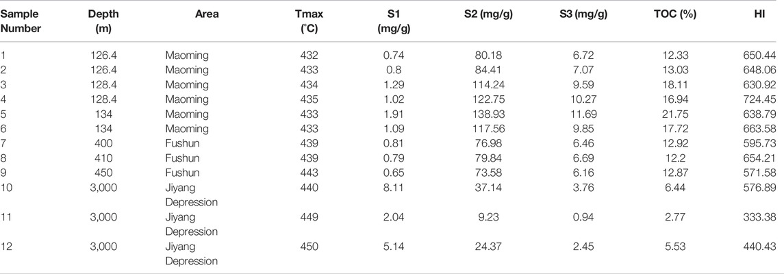
TABLE 1. The initial geochemical parameters of the samples.

FIGURE 1

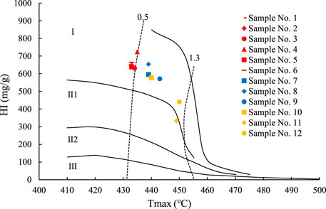
FIGURE 1. Tmax versus HI diagram of samples.

The characteristics of the thermal simulation products were affected by the maturity. Samples 10–12 have higher maturities, and the hydrocarbon generation occurred later than for the nine immature–low maturity samples. Under the same temperature conditions, the conversion rate of the mature shale samples was lower than that of the other immature–low maturity oil shale samples (Figure 2). This demonstrates that oil shale/shale oil with a higher maturity requires higher temperature conditions for in situ conversion.

FIGURE 2

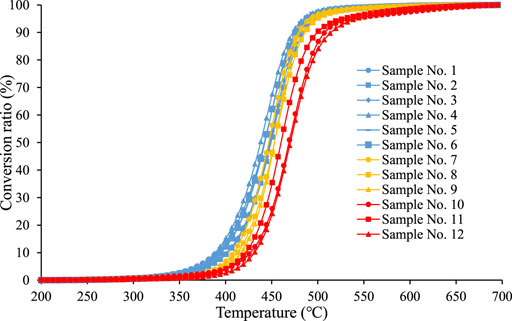
FIGURE 2. Hydrocarbon generation conversion curves of the open system experiment.

It can be seen from the results of the open system experiment that the heavy hydrocarbons (C₁₄₊) generation period was the shortest, occurring at temperatures of 370–500°C, followed by the light hydrocarbons (C_6–14) generation period at temperatures of 340–520°C; the gaseous hydrocarbons (C_1–5) generation period was the longest, occurring at temperatures of 300–650°C (Figure 3). According to the closed system thermal simulation results, the C_1–5 yield continuously increased, and the lower the heating rate, the higher the C_1–5 yield at the same temperature. Both the C_6–14 and C₁₄₊ components underwent secondary cracking. The lower the heating rate, the lower the temperature at which the secondary cracking occurred (Figure 4).

FIGURE 3

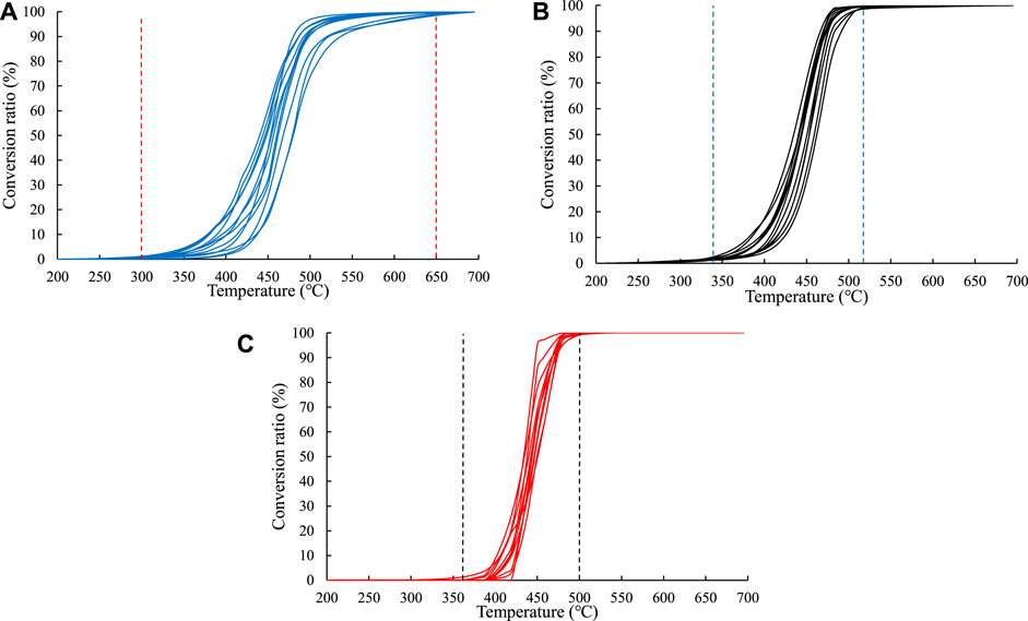
FIGURE 3. Hydrocarbon generation conversion rates at different temperatures in the open system experiments. (A) C_1–5. (B) C_6–14. (C) C₁₄₊.

FIGURE 4

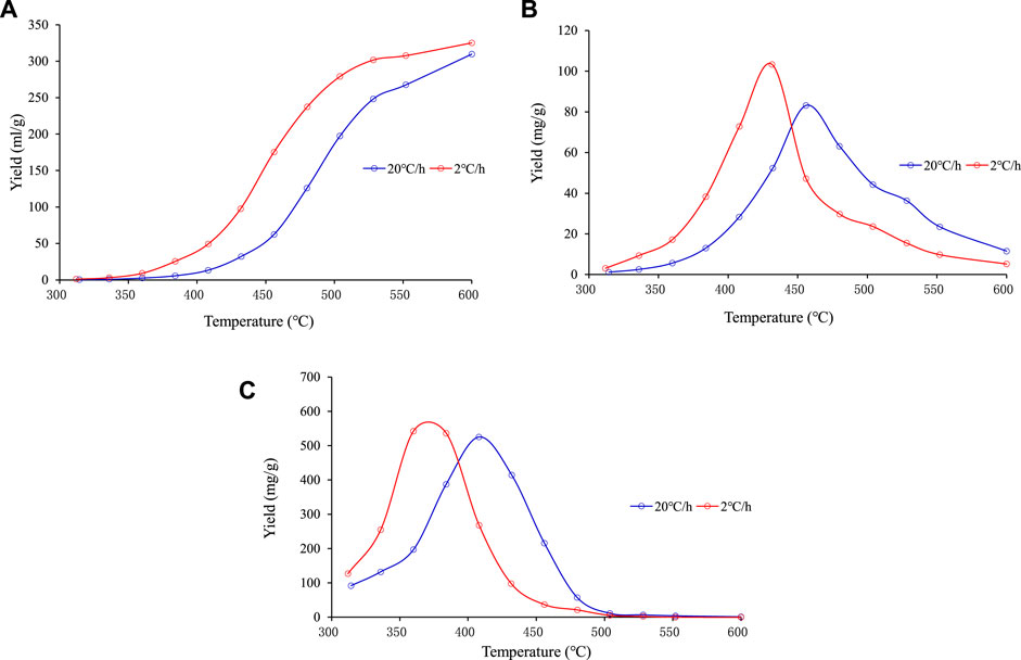
FIGURE 4. Hydrocarbon generation conversion rate at different temperatures of sample No. Nine in the closed system experiments. (A) C_1–5. (B) C_6–14. (C) C₁₄₊.

By comparing the results of the liquid hydrocarbon (C_6–14 and C₁₄₊) conversion in the open system experiments and the closed system experiments, it was found that the results of heavy hydrocarbons conversion in the two systems were basically the same when EasyRo <1% (Figure 5).

FIGURE 5

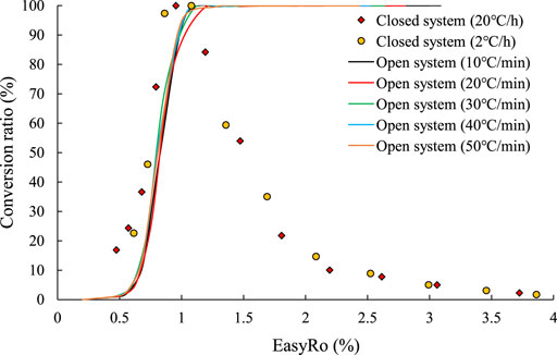
FIGURE 5. Comparison of the conversion ratio of the liquid hydrocarbons in the open system and closed system experiments.

3 Model Calibration and Application

3.1 Model Calibration

3.1.1 Construct the Objective Function

Assuming that at a certain heating rate l, when a certain temperature j is reached, the hydrocarbon production rate measured in the experiment is X1_lj. Under the same conditions, assuming E_i, A_i, and X_i0, the hydrocarbon production rate calculated using the model is X_lj. If there is a certain group of E_i, A_i, and X_i0 values such that X1_lj − X_lj = 0 for all l and j, then this group of E_i, A_i, and X_i0 values represents the correct parameters. However, due to experimental errors and other reasons, this is actually impossible. Therefore, the values of E_i, A_i, and X_i0 that make X1_lj − X_lj as small as possible are the substitutes. Thus, the objective function can be constructed as Eq 8 to characterize the calculation error.

$Q\left(A,X\right)={\displaystyle \sum _{l=1}^{L0}{\displaystyle {\sum }_{j=1}^{J0}{\left(X{1}_{\mathrm{l}\mathrm{j}}-X_{lj}\right)}^2}}(8)$

where L0 is the number of experiments with different heating rates, and J0 is the number of sampling points from an experimental curve.

In addition, for each parameter in the formula, certain constraints listed in Eq 9 must be met. E_i can be solved by determining the distribution range of the activation energy of the parallel reactions and the activation energy interval of the adjacent parallel reactions.

$\{\begin{array}{l}{A}_i>0\\ 0\le X_{i0}\le 1\\ {\displaystyle \sum _{i=1}^N{X}_{i0}=1\mathrm{ }\mathrm{o}\mathrm{r}\mathrm{ }|1-{\displaystyle \sum _{i=1}^N{X}_{i0}}|\le \epsilon \left(\epsilon isa\inf initely\mathrm{ }small\mathrm{ }positivenumber\right)}\end{array}(9)$

Thus far, the problem of obtaining the kinetic parameters has been changed to the problem of finding the minimum point at which the non–negative objective function satisfies the constraint conditions.

3.1.2 Construct the Penalty Function

The abovementioned problem of finding the minimum value that satisfies the constraint conditions is more complicated because in addition to the gradual decrease in the value of the objective function, attention must be paid to the feasibility of the solution, that is, to determine whether the solution is within the range defined by the constraint conditions. Thus, the penalty function method is adopted to turn the constrained extreme value problem into an unconstrained extreme value problem. The process is as follows.

For any constraint condition, a function can be constructed. When the obtained extreme point meets the condition, the function’s value is 0; otherwise, it is a positive number.

If A_i > 0, this constraint condition can be obtained as follows:

$G_1\left(A_i\right)=\{\begin{array}{c}0\mathrm{ }\mathrm{w}\mathrm{h}\mathrm{e}\mathrm{n}\mathrm{ }A\ge 0\\ {{\rm A}}_i^2\mathrm{ }\mathrm{w}\mathrm{h}\mathrm{e}\mathrm{n}\mathrm{ }A\le 0\end{array}(10)$

That is,G₁ (A_i) = [min(0, A_i]². For the other constraints, the method is the same as for A_i. Because of space limitations, the constraints on the remaining parameters are not repeated here. After the penalty function of each constraint condition is constructed, the penalty items can be obtained as follows:

$\begin{array}{l}{G}_1\left(A_i,X_{i0}\right)=G_1+G_2+G_3\\ \mathrm{ }={\left[\min \left(0,A_i\right)\right]}^2+{\left[\min \left(0,X_{i0}\right)\right]}^2+{\left[\min \left(\mathrm{0,1}-X_{i0}\right)\right]}^2+\left[\min \left(0,\epsilon -\left|1-{\displaystyle \sum _{i=1}^N{X}_{i0}}\right|\right)\right]\end{array}(11)$

Use a sufficiently large positive integer R to construct a penalty function

$F\left(A{}_i,X_{i0}\right)=Q\left(A{}_i,X_{i0}\right)+R\cdot G\left(A{}_i,X_{i0}\right)(12)$

If the obtained minimum point exceeds the constraint condition, the coefficient R is gradually increased. When R is sufficiently large, the minimum solution of the penalty term is the minimum solution of the objective function, thus turning the constrained extreme value problem into unconstrained extreme value problems, which are relatively easy to solve.

3.1.3 Calculate the First–Order Partial Derivative

The necessary condition for the existence of the minimum is that the first–order partial derivative of the penalty function is 0.

First find the partial derivative of the objective function:

$\frac{\partial Q}{\partial A_m}={\displaystyle \sum _{l=1}^{L0}{\displaystyle \sum _{j=1}^{J0}\left(-2\left(X{1}_{lj}-X_{lj}\right)\cdot \frac{\partial X_{lj}}{\partial A_m}\right)}}(13)$

where

$\frac{\partial X_{lj}}{\partial A_m}=\frac{\partial {\displaystyle \sum _{i=1}^N\left(X_{i0}\left(1-\exp \left(-{\displaystyle {\int }_{T_0}^{T_{\mathrm{l}\mathrm{j}}}\frac{A_i}{D_l}\exp }\left(-\frac{E_i}{RT}\right)dT\right)\right)\right)}}{\partial A_m}(14)$

When i≠m, partial derivative is 0, so,

$\frac{\partial X_{lj}}{\partial A_m}=X_{m0}\cdot \exp \left(-{\displaystyle {\int }_{T_0}^{T_{lj}}\frac{A_m}{D_l}\exp \left(-\frac{E_m}{RT}\right)dT}\right)\cdot {\displaystyle {\int }_{T_0}^T\frac{1}{D_l}\exp \left(-\frac{E_m}{RT}\right)dT}(15)$

$\begin{array}{l}\frac{\partial Q}{\partial X_{m0}}={\displaystyle \sum _{l=1}^{L0}{\displaystyle \sum _{j=1}^{J0}\left(-2\left(X{1}_{lj}-X_{lj}\right)\cdot \frac{\partial X_{lj}}{\partial X_{m0}}\right)}}\\ ={\displaystyle \sum _{l=1}^{L0}{\displaystyle \sum _{j=1}^{J0}\left(-2\left(X{1}_{lj}-X_{lj}\right)\cdot \left(1-\exp \left(-{\displaystyle {\int }_{T_0}^{T_{lj}}\frac{A_m}{D_l}}\exp \left(-\frac{E_m}{RT}\right)dT\right)\right)\right)}}\end{array}(16)$

m = 1, 2, 3, … , N.

partial derivatives of the penalty term are as follows:

$\frac{\partial G}{\partial A_m}=2\cdot \min \left(0,A_m\right)(17)$

$\frac{\partial G}{\partial X_{m0}}=2\cdot \min \left(0,X_{m0}\right)-2\cdot \min \left(\mathrm{0,1}-X_{m0}\right)-2\cdot \min \left(0,\epsilon -\left|1-{\displaystyle \sum _{i=1}^N{X}_{i0}}\right|\right)\cdot \mathrm{F}\mathrm{N}\left({\displaystyle \sum _{i=1}^N{X}_{i0}-1}\right)(18)$

FN means:

$\mathrm{F}\mathrm{N}\left({\displaystyle {\sum }_{i=1}^N{X}_{i0}-1}\right)=\{\begin{array}{c}1\mathrm{ }\mathrm{w}\mathrm{h}\mathrm{e}\mathrm{n}\mathrm{ }{\displaystyle {\sum }_{i=1}^N{X}_{i0}-1>0}\\ -1\mathrm{ }\mathrm{w}\mathrm{h}\mathrm{e}\mathrm{n}\mathrm{ }{\displaystyle {\sum }_{i=1}^N{X}_{i0}-1<0}\end{array}(19)$

m = 1, 2, 3, … , N

Obtain the partial derivative of the objective function and the penalty term. After the partial derivative is obtained, theoretically speaking, the minimum point should meet the following conditions:

$\{\begin{array}{l}\frac{\partial F\left(A_i,X_{i0}\right)}{\partial A{O}_m}=\frac{\partial Q}{\partial A_m}+R1\cdot \frac{\partial G}{\partial A_m}=0\\ \frac{\partial F\left(A_i,X_{i0}\right)}{\partial X_{m0}}=\frac{\partial Q}{\partial X_{m0}}+R1\cdot \frac{\partial G}{\partial X_{m0}}=0\end{array}(20)$

m = 1, 2, 3, … , N

Therefore, if the equations can be obtained accurately, several possible minima can be obtained, which can be used to solve for the 2 × N undetermined kinetic parameters (A_i, X_i0) and to complete the model calibration. Although it is impossible to find an exact solution for such a complex non–polynomial function as the above equations, an approximate solution can be found.

3.1.4 Approximate the Minima

A variety of optimization algorithms are available to solve the unconstrained value problem. In this study, the variable–scaling method with fast convergence speed and no need to calculate the cumbersome second derivative matrix and its inverse matrix was selected for the optimization calculation. The detailed derivation of the variable–scale optimization algorithm can be found in the literature (Powell, 1978).

When calibrating the overall reaction model, the difference from the parallel first–order reaction is the change in the order of the reaction (n) and the change in the constraint conditions.

Compared with the parallel first–order reaction model, the constraints of the overall reaction model are as follows:

$\{\begin{array}{l}E>0\\ A>0\\ n>0\end{array}(21)$

In addition, the corresponding penalties are as follows:

$G\left(A,E,n\right)=G_1+G_2+G_3={\left[\min \left(0,A\right)\right]}^2+{\left[\min \left(0,E\right)\right]}^2+{\left[\min \left(0,n\right)\right]}^2(22)$

$F\left(A,E,\mathrm{n}\right)=Q\left(A,E,\mathrm{n}\right)+R1\cdot G\left(A,E,\mathrm{n}\right)(23)$

The partial derivative of the objective function to the activation energy is as follows:

$\begin{array}{l}\frac{\partial Q}{\partial E}={\displaystyle \sum _{l=1}^{L0}{\displaystyle \sum _{j=1}^{J0}\left(-2\left(X{1}_{lj}-X_{lj}\right)\cdot \frac{\partial X_{lj}}{\partial E}\right)}}\\ \mathrm{ }={\displaystyle \sum _{l=1}^{L0}{\displaystyle \sum _{j=1}^{J0}2\left(X{1}_{lj}-X_{lj}\right)\cdot {\left(1-\left(1-n\right){\displaystyle {\int }_{T0}^{T_{lj}}\frac{A}{D}\exp \left(-\frac{E}{RT}\right)}dT\right)}^{\frac{n}{1-n}}\cdot {\displaystyle {\int }_{T0}^{T_{lj}}\frac{A}{D}\cdot \frac{1}{RT}\exp \left(-\frac{E}{RT}\right)}dT\left(n\ne 1\right)}}\end{array}(24)$

$\begin{array}{l}\frac{\partial Q}{\partial E}={\displaystyle \sum _{l=1}^{L0}{\displaystyle \sum _{j=1}^{J0}\left(-2\left(X{1}_{lj}-X_{lj}\right)\cdot \frac{\partial X_{lj}}{\partial E}\right)}}\\ ={\displaystyle \sum _{l=1}^{L0}{\displaystyle \sum _{j=1}^{J0}\left(2\left(X{1}_{lj}-X_{lj}\right)\cdot \exp \left(-{\displaystyle {\int }_{T0}^{T_{lj}}\frac{A}{D}\exp \left(-\frac{E}{RT}\right)}dT\right)\cdot {\displaystyle {\int }_{T0}^{T_{lj}}\frac{A}{D}\cdot \left(\frac{1}{RT}\right)\cdot \exp \left(-\frac{E}{RT}\right)}dT\right)}}\left(n=1\right)\end{array}(25)$

The partial derivative of the objective function to the frequency factor as follows:

$\frac{\partial Q}{\partial A}={\displaystyle \sum _{l=1}^{L0}{\displaystyle \sum _{j=1}^{J0}\left(-2\left(X{1}_{lj}-X_{lj}\right)\cdot \frac{\partial X_{lj}}{\partial A}\right)}}(26)$

where

$\begin{array}{c}\frac{\partial X_{lj}}{\partial A}=\frac{\partial \left(1-{\left(1-\left(1-n\right){\displaystyle {\int }_{T0}^{T_{lj}}\frac{A}{D}\exp \left(-\frac{E}{RT}\right)}dT\right)}^{\frac{1}{1-n}}\right)}{\partial AO}\\ ={\left(1-\left(1-n\right){\displaystyle {\int }_{T0}^{T_{lj}}\frac{A}{D}\exp \left(-\frac{E}{RT}\right)}dT\right)}^{\frac{n}{1-n}}\cdot {\displaystyle {\int }_{T0}^{T_{lj}}\frac{1}{D}\exp \left(-\frac{E}{RT}\right)}dT\left(\mathrm{n}\ne 1\right)\end{array}(27)$

$\begin{array}{c}\frac{\partial X_{lj}}{\partial A}=\frac{\partial \left(1-\exp \left(-{\displaystyle {\int }_{T0}^{T_{lj}}\frac{A}{D}\exp \left(-\frac{E}{RT}\right)}dT\right)\right)}{\partial AO}\\ =\exp \left(-{\displaystyle {\int }_{T0}^{T_{lj}}\frac{A}{D}\exp \left(-\frac{E}{RT}\right)}dT\right)\cdot \left({\displaystyle {\int }_{T0}^{T_{lj}}\frac{1}{D}\exp \left(-\frac{E}{RT}\right)}dT\right)\left(\mathrm{n}=1\right)\end{array}(28)$

The partial derivative of the objective function to the order of the reaction is as follows:

$\frac{\partial Q}{\partial n}={\displaystyle \sum _{l=1}^{L0}{\displaystyle \sum _{j=1}^{J0}\left(-2\left(X{1}_{lj}-X_{lj}\right)\cdot \frac{\partial X_{lj}}{\partial n}\right)}}(29)$

where

$\begin{array}{l}\frac{\partial X_{lj}}{\partial n}=-{\left[1-\left(1-n\right){\displaystyle {\int }_{T0}^{T_{lj}}\frac{A}{D}}\exp \left(\frac{-E}{RT}\right)\mathrm{d}T\right]}^{\frac{1}{1-n}}\\ \mathrm{ }\cdot \left[\begin{array}{l}\ln \left(1-\left(1-n\right)\right){\displaystyle {\int }_{T0}^{T_{lj}}\frac{A}{D}}\exp \left(\frac{-E}{RT}\right)\mathrm{d}\mathrm{T)}\cdot {\left(\frac{1}{1-n}\right)}^2+\\ {\displaystyle {\int }_{T0}^{T_{lj}}\frac{A}{D}}\exp \left(\frac{-E}{RT}\right)\mathrm{d}T\cdot {\left(1-\left(1-n\right){\displaystyle {\int }_{T0}^{T_{lj}}\frac{A}{D}}\exp \left(\frac{-E}{RT}\right)\mathrm{d}T\right)}^{-1}\cdot \frac{1}{1-n}\end{array}\right]\left(n\ne 1\right)\end{array}(30)$

When n = 1, there is no need to calculate the partial derivative of the objective function to the order of the reaction.

The partial derivative of the penalty term is as follows:

$\frac{\partial Q}{\partial A}=2\cdot \min \left(0,A\right)(31)$

$\frac{\partial Q}{\partial E}=2\cdot \min \left(0,E\right)(32)$

$\frac{\partial G}{\partial n}=2\cdot \min \left(0,\mathrm{n}\right)(33)$

After obtaining the partial derivatives of A, E, and n, the subsequent optimization of the activation energy at the minimum point of the objective function, the frequency factor, and the reaction order are the same as for the parallel first–order reaction model.

3.2 Model Application

Figure 6 shows the comparison of the fitting effects of the parallel first–order reaction model and the overall nth–order reaction model for sample No. Nine in the open system experiment. Figure 7 shows the comparison of the average calculation errors of the parallel first–order reaction model and the overall nth–order reaction model for all of the calculated values of the samples. The two models have different fitting effects for the different hydrocarbon generation reactions. For the fitting effects of the generation of C_1–5 from organic matter and the generation of C_6–14 from organic matter, the average calculation error of the parallel first–order reaction model is smaller than that of the overall nth–order reaction model. For the generation of C₁₄₊ from organic matter, the average calculation error of the overall nth–order reaction model is smaller than that of the parallel first–order reaction model.

FIGURE 6

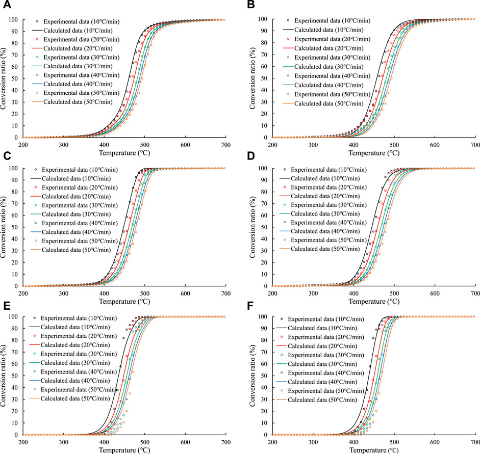
FIGURE 6. Comparison of the fitting effects of the parallel first–order reaction model and the overall nth–order reaction model on experimental data of sample No. Nine in the open system experiments. Figures 6A, C, E are the fitting effect of the parallel first–order reaction on the generation of C_1–5, C_6–14 and C₁₄₊, respectively; Figures 6B, D, F are the fitting effect of the overall nth–order reaction on the generation of C_1–5, C_6–14 and C₁₄₊, respectively.

FIGURE 7

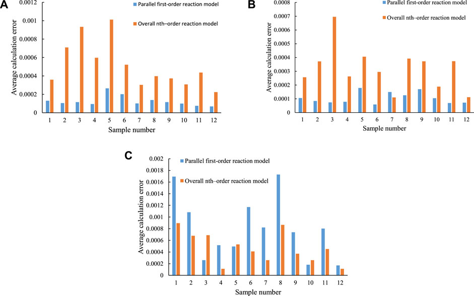
FIGURE 7. Comparison of the average calculation errors of the parallel first–order reaction model and the overall nth–order reaction model. (A) C_1–5. (B) C_6–14. (C) C₁₄₊.

Figures 8, 9 show the fitting effects of the parallel first–order reaction model and the overall nth–order reaction model on the measured values of the closed system experiment. It can be seen that the fitting effect of the parallel first–order reaction model is better than the overall nth–order reaction model.

FIGURE 8

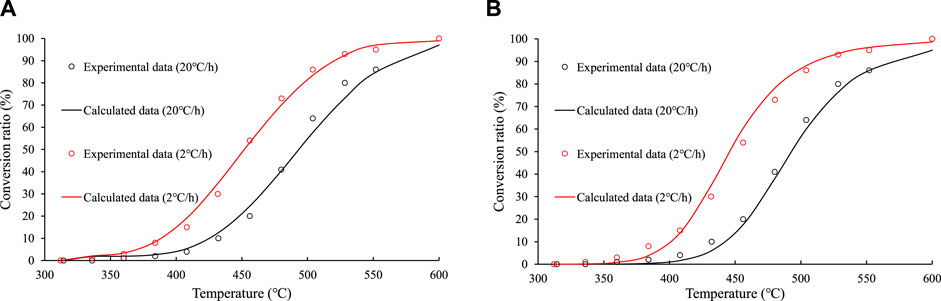
FIGURE 8. Comparison of the fitting effects of the parallel first–order reaction model and the overall nth order reaction model on experimental data of the gas hydrocarbon in the closed system experiments on sample No. 9. (A) parallel first–order reaction model. (B) overall nth–order reaction model.

FIGURE 9

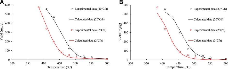
FIGURE 9. Comparison of the fitting effects of the parallel first–order reaction model and the overall nth–order reaction model on experimental data of the liquid hydrocarbon in the closed system experiments on sample No. 9. (A) parallel first–order reaction model. (B) overall nth–order reaction model.

Figure 10 shows the distribution diagrams of the calculated reaction activation energies of the different reactions in the different systems. The standard deviation (σ) was selected to reflect the degree of dispersion of the activation energy, and a smaller standard deviation represents a more discrete activation energy distribution. The standard deviation equation is as follows:

$\sigma =\sqrt{\frac{{\displaystyle {\sum }_{\mathrm{i}=1}^n{\left(e_i-\overline{e}\right)}^2}}{n}}(34)$

where e_i is the ratio of activation energy of each reaction to the total reaction, and $\stackrel{\_}{e}$ is the average of e_i.

FIGURE 10

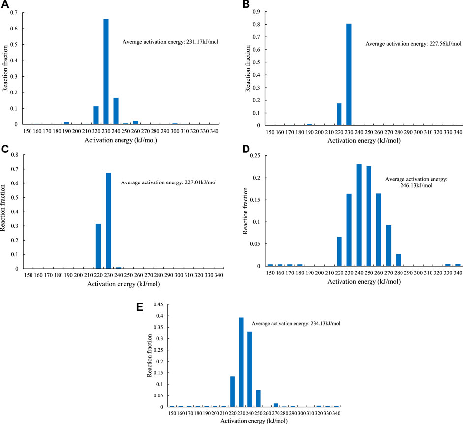
FIGURE 10. The activation energy distribution of hydrocarbon generation from the pyrolysis of sample No. 9. (A) C_1–5 generation in the open system. (B) generation of C_6–14 in the open system. (C) generation of C₁₄₊ in the open system. (D) C_1–5 generation in the closed system. (E) liquid hydrocarbon cracking in the closed system.

As can be seen from Figures 10, 11, the activation energy distribution of the C_1–5 is the most dispersed, with σ ranging from 0.107 to 0.157. The σ range of activation energy distribution of the C_6–14 is 0.132–0.185. The activation energy distribution of the C₁₄₊ is the most concentrated, with a σ range of 0.147–0.189. In addition, the activation energy distribution of the closed system is more dispersed than that of open system, with σ of 0.080 and an average activation energy of 246.13 kJ/mol, which are higher than those of the open system reaction.

FIGURE 11

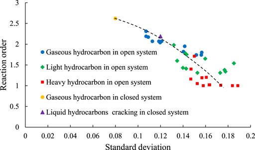
FIGURE 11. Reaction order and standard deviation of different hydrocarbon generation reactions.

As can be seen from the trend of the reaction orders of the different reactions, the reaction order of the generation reaction of the C_1–5 is the largest, ranging from 1.74 to 2.31 (mean 2.00). The reaction order of the generation reaction of the C₁₄₊ is the smallest, ranging from 1.00 to 1.71 (mean 1.15). The reaction order of the generation reaction of the C_6–14 is between those of the gaseous hydrocarbons and the heavy hydrocarbons, ranging from 1.31 to 1.98 (mean 1.54) (Figure 11). The reaction order of generation reaction of C_1–5 in the closed system is 2.62, which is biggest among all of the reactions.

4 Discussion

4.1 Effect of Organic Matter Maturity on Activation Energy

The activation energy of hydrocarbon generation reflects the difficulty of the organic matter cracking and hydrocarbon generation. The higher the maturity, the higher the activation energy of the reaction. Tmax exhibits a good correlation with maturity. According to the pyrolysis information and kinetic parameters of the 12 samples analyzed in this study, for any organic matter hydrocarbon generation reaction, there is a positive correlation between the Tmax and activation energy (Figure 12). It can be seen that the higher the maturity, the higher the peak temperature of the pyrolysis and the higher the activation energy of the reaction, which causes the lag in the hydrocarbon generation period (Figure 2).

FIGURE 12

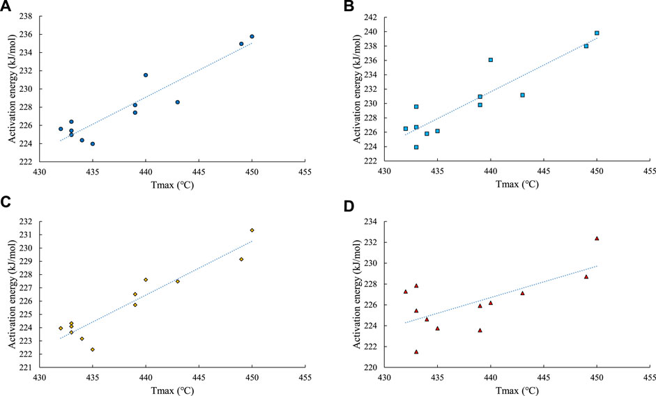
FIGURE 12. The relationship between the activation energy of hydrocarbon generation in the open system and Tmax. (A) total hydrocarbons from organic matter. (B) generation of C_1–5 from organic matter. (C) generation of C_6–14 from organic matter. (D) generation of C₁₄₊ from organic matter.

4.2 Influence of the Hydrocarbon Generation Period on the Model Fitting Effect

The parallel first–order reaction model uses different reactions to characterize the different reaction stages. For reactions with longer reaction periods such as the generation of gaseous hydrocarbons and light hydrocarbons from organic matter in an open system and the generation of gaseous hydrocarbons from organic matter in a closed system, the parallel first–order response model has a better fitting effect. The overall reaction model uses only one reaction to describe the entire reaction process. In order to achieve the best fitting effect, the model prioritizes the optimization of the main phase of the reaction, and the initial and final stages of the reaction have poor fitting effects. For reactions such as the generation of heavy hydrocarbons from organic matter, which has a short reaction period, the nth–order reactions have an advantage in the fitting process, and compared with first–order reactions, the fitting effect is better.

4.3 Influence of the Hydrocarbon–Generating Parent Material on the Order of the Reaction

Kerogen is a complex polycondensate polymer with no fixed chemical composition and only a certain range of compositions (Tissot and Deroo, 1978; Pavle et al., 1998; Love et al., 1998). Kerogen is mainly composed of three groups (aliphatic structure, aromatic structure, and heteroatom structure), among which the aliphatic structure and aromatic structure are the main groups that generate the hydrocarbons and gases, and each group includes a variety of compounds with different chemical formulas. In the process of generating hydrocarbons from organic matter, compounds with different molecular formulas can generate hydrocarbons when heated, and the hydrocarbon generation from each compound can be regarded as a sub–reaction of the total reaction of the hydrocarbon generation from the kerogen.

The order of the reaction is the sum of the orders of the sub–reactions. Therefore, the more diverse sub–reactions, the higher reaction order. In the generation of hydrocarbons from organic matter, the gas generation reaction runs through the entire evolution stage. In addition to the direct generation of gaseous hydrocarbons from the organic matter, the secondary cracking of liquid hydrocarbons in the later stage of pyrolysis can also produce gaseous hydrocarbons, that is, the parent material types of the gaseous hydrocarbon components are the most diverse. As a result, the gas generation process of organic matter contains the most chemical reactions, and the reaction order is the highest, followed by the light hydrocarbons. Heavy hydrocarbon components are generated from the fewest types of parent material and have the lowest reaction order. The activation energy distributions of the different components calculated using the parallel reaction model and the order of the reaction characteristics of each component calculated using the overall nth–order reaction model exhibit the uniformity of hydrocarbon generation mechanism, which shows the rationality and accuracy of the models.

5 Conclusion

Based on the characterization results of the pyrolysis kinetics of continental shale obtained using the two models, the following conclusions were drawn.

The parallel first–order reaction model characterizes the reaction diversity based on the number and distribution characteristics of the parallel reactions, while the overall nth–order reaction model characterizes the reaction diversity based on the change in the order of the reaction. The combination of the two models can be used to better explore the hydrocarbon generation reaction mechanism.

The activation energies of the continental shale samples with different maturities were different. The higher the maturity of the sample, the higher the activation energy of the hydrocarbon generation, the more the hydrocarbon generation lagged, and the higher the temperature required for the in situ conversion process.

The parallel first–order reaction model decomposes the hydrocarbon generation reaction into a series of parallel first–order reactions. For various reactions with longer reaction periods, such as the generation of C_1–5 and C_6–14 from organic matter in the closed system, the reaction fitting effect is better. Due to the rationality of the reaction order setting, the overall nth–order reaction model has a better fitting effect for reactions with shorter reaction periods, such as the generation of C₁₄₊ from organic matter.

The order of the reaction is the sum of the orders of the sub–reactions. In the hydrocarbon generation reaction, the more complex the type of parent material, the larger the number of reactions and the larger the order of the reaction. Thus, the reaction order of C_1–5 generation is highest, the second is the generation of C_6–14, and the last is generation of C₁₄₊.

Data Availability Statement

The original contributions presented in the study are included in the article/Supplementary Material, further inquiries can be directed to the corresponding author.

Author Contributions

JJ: Writing—Original Draft Preparation JL: Writing—Review and Editing, Supervision, Funding acquisition YW: Conceptualization, Project administration XC: Methodology, Project administration MW: Formal analysis, Project administration SL: Investigation, Project administration HY: Project administration KZ: Methodology, Visualization CY: Software, Validation ZL: Project administration LY: Resources, Data curation.

Funding

Our funding comes from the National Natural Science Foundation of China, which mainly provides funding for basic theoretical research. This study was supported by the National Natural Science Foundation of China (No. 42172145).

Conflict of Interest

Authors YW and XC were employed by Sinopec Petroleum Exploration and Production Research Institute. ZL was employed by China United Coalbed Methane Corporation Ltd. LY was employed by PetroChina JiLin Oilfield Company.

The remaining authors declare that the research was conducted in the absence of any commercial or financial relationships that could be construed as a potential conflict of interest.

Publisher’s Note

All claims expressed in this article are solely those of the authors and do not necessarily represent those of their affiliated organizations, or those of the publisher, the editors and the reviewers. Any product that may be evaluated in this article, or claim that may be made by its manufacturer, is not guaranteed or endorsed by the publisher.

Acknowledgments

The authors would like to thank the editors and reviewers for their valuable suggestions for this paper.

References

Allred, V. D. (1966). Kinetics of Oil Shale Pyrolysis. Chem. Eng. Prog. 62, 55–60.

Google Scholar

Behar, F., Vandenbroucke, M., Tang, Y., Marquis, F., and Espitalie, J. (1997). Thermal Cracking of Kerogen in Open and Closed Systems: Determination of Kinetic Parameters and Stoichiometric Coefficients for Oil and Gas Generation. Org. Geochem. 26 (5–6), 321–339. doi:10.1016/s0146-6380(97)00014-4

CrossRef Full Text | Google Scholar

Behar, F., Lorant, F., and Lewan, M. (2008). Role of NSO Compounds during Primary Cracking of a Type II Kerogen and a Type III lignite. Org. Geochem. 39 (1), 1–22. doi:10.1016/j.orggeochem.2007.10.007

CrossRef Full Text | Google Scholar

Brandt, A. R. (2008). Converting Oil Shale to Liquid Fuels: Energy Inputs and Greenhouse Gas Emissions of the Shell In Situ Conversion Process. Environ. Sci. Technol. 42 (19), 7489–7495. doi:10.1021/es800531f

PubMed Abstract | CrossRef Full Text | Google Scholar

Braun, R. L., and Burnham, A. K. (1987). Analysis of Chemical Reaction Kinetics Using a Distribution of Activation Energies and Simpler Models. Energy Fuels 1 (2), 153–161. doi:10.1021/ef00002a003

CrossRef Full Text | Google Scholar

Burnham, A. K., Schmidt, B. J., and Braun, R. L. (1995). A Test of the Parallel Reaction Model using Kinetic Measurements on Hydrous Pyrolysis Residues. Organ. Geochem. 23 (10), 931–939. doi:10.1016/0146-6380(95)00069-0

CrossRef Full Text | Google Scholar

Burnham, A. K., and Braun, R. L. (1999). Global Kinetic Analysis of Complex Materials. Energy Fuels 13 (1), 1–22. doi:10.1021/ef9800765

CrossRef Full Text | Google Scholar

Burnham, A. K., and Sweeney, J. J. (1989). A Chemical Kinetic Model of Vitrinite Maturation and Reflectance. Geochimica et Cosmochimica Acta 53 (10), 2649–2657. doi:10.1016/0016-7037(89)90136-1

CrossRef Full Text | Google Scholar

Chen, J., Zhang, X., Chen, Z., Pang, X., Yang, H., Zhao, Z., et al. (2021). Hydrocarbon Expulsion Evaluation Based on Pyrolysis Rock-Eval Data: Implications for Ordovician Carbonates Exploration in the Tabei Uplift, Tarim. J. Pet. Sci. Eng. 196, 107614. doi:10.1016/j.petrol.2020.107614

CrossRef Full Text | Google Scholar

Chen, Z., Lavoie, D., Mort, A., Jiang, C., Zhang, S., Liu, X., et al. (2020). Source Rock Kinetics and Petroleum Generation History of the Upper Ordovician Calcareous Shales of the Hudson Bay Basin and Surrounding Areas. Fuel 270, 117503. doi:10.1016/j.fuel.2020.117503

CrossRef Full Text | Google Scholar

Chen, Z., Li, M., Cao, T., Ma, X., Li, Z., Jiang, Q., et al. (2017a). Hydrocarbon Generation Kinetics of a Heterogeneous Source Rock System: Example from the Lacsutrine Eocene-Oligocene Shahejie Formation, Bohai Bay Basin, China. Energy Fuels 31 (12), 13291–13304. doi:10.1021/acs.energyfuels.7b02361

CrossRef Full Text | Google Scholar

Chen, Z., Liu, X., Guo, Q., Jiang, C., and Mort, A. (2017b). Inversion of Source Rock Hydrocarbon Generation Kinetics from Rock-Eval Data. Fuel 194, 91–101. doi:10.1016/j.fuel.2016.12.052

CrossRef Full Text | Google Scholar

Chen, Z., Liu, X., and Jiang, C. (2017c). Quick Evaluation of Source Rock Kerogen Kinetics Using Hydrocarbon Pyrograms from Regular Rock-Eval Analysis. Energy Fuels 31 (2), 1832–1841. doi:10.1021/acs.energyfuels.6b01569

CrossRef Full Text | Google Scholar

Dieckmann, V. (2005). Modelling Petroleum Formation from Heterogeneous Source Rocks: the Influence of Frequency Factors on Activation Energy Distribution and Geological Prediction. Mar. Pet. Geology. 22 (3), 375–390. doi:10.1016/j.marpetgeo.2004.11.002

CrossRef Full Text | Google Scholar

Haddadin, R. A., and Tawarah, K. M. (1980). DTA Derived Kinetics of Jordan Oil Shale. Fuel 59, 539–543. doi:10.1016/0016-2361(80)90187-8

CrossRef Full Text | Google Scholar

Han, S., Horsfield, B., Zhang, J., Chen, Q., Mahlstedt, N., di Primio, R., et al. (2014). Hydrocarbon Generation Kinetics of Lacustrine Yanchang Shale in Southeast Ordos Basin, North China. Energy Fuels 28 (9), 5632–5639. doi:10.1021/ef501011b

CrossRef Full Text | Google Scholar

Hazra, B., Dutta, S., and Kumar, S. (2017). TOC Calculation of Organic Matter Rich Sediments Using Rock-Eval Pyrolysis: Critical Consideration and Insights. Int. J. Coal Geology. 169, 106–115. doi:10.1016/j.coal.2016.11.012

CrossRef Full Text | Google Scholar

He, W., Sun, Y., Guo, W., and Shan, X. (2021). Controlling the In-Situ Conversion Process of Oil Shale via Geochemical Methods: A Case Study on the Fuyu Oil Shale, China. Fuel Process. Techn. 219, 106876. doi:10.1016/j.fuproc.2021.106876

CrossRef Full Text | Google Scholar

Hill, R. J., Tang, Y., and Kaplan, I. R. (2003). Insights into Oil Cracking Based on Laboratory Experiments. Org. Geochem. 34 (12), 1651–1672. doi:10.1016/s0146-6380(03)00173-6

CrossRef Full Text | Google Scholar

Johnson, L. M., Rezaee, R., Smith, G. C., Mahlstedt, N., Edwards, D. S., Kadkhodaie, A., et al. (2020). Kinetics of Hydrocarbon Generation from the marine Ordovician Goldwyer Formation, Canning Basin, Western Australia. Int. J. Coal Geology. 232, 103623. doi:10.1016/j.coal.2020.103623

CrossRef Full Text | Google Scholar

Kang, Z., Zhao, Y., and Yang, D. (2020). Review of Oil Shale In-Situ Conversion Technology. Appl. Energ. 269, 115121. doi:10.1016/j.apenergy.2020.115121

CrossRef Full Text | Google Scholar

Klomp, U. C., and Wright, P. A. (1990). A New Method for the Measurement of Kinetic Parameters of Hydrocarbon Generation from Source Rocks. Org. Geochem. 16 (1), 49–60. doi:10.1016/0146-6380(90)90025-u

CrossRef Full Text | Google Scholar

Li, M., Chen, Z., Ma, X., Cao, T., Li, Z., and Jiang, Q. (2018). A Numerical Method for Calculating Total Oil Yield Using a Single Routine Rock-Eval Program: A Case Study of the Eocene Shahejie Formation in Dongying Depression, Bohai Bay Basin, China. Int. J. Coal Geology. 191, 49–65. doi:10.1016/j.coal.2018.03.004

CrossRef Full Text | Google Scholar

Love, G. D., Snape, C. E., and Fallick, A. E. (1998). Differences in the Mode of Incorporation and Biogenicity of the Principal Aliphatic Constituents of a Type I Oil Shale. Org. Geochem. 28 (12), 797–811. doi:10.1016/s0146-6380(98)00050-3

CrossRef Full Text | Google Scholar

Pavle, I. P., Ivana, R. T., Mirjana, S. P., Liliana, L., and Salvador, L. (1998). Classification of the Asphalts and Their Source Rock from the Dead Sea Basin (Israel): the Asphaltene/kerogen Vanadyl Porphyrins. Fuel 77 (15), 1769–1776.

Google Scholar

Pepper, A. S., and Corvi, P. J. (1995). Simple Kinetic Models of Petroleum Formation. Part I: Oil and Gas Generation from Kerogen. Mar. Pet. Geology. 12 (3), 291–319. doi:10.1016/0264-8172(95)98381-e

CrossRef Full Text | Google Scholar

Powell, M. J. D. (1978). The Convergence of Variable Metric Methods for Nonlinearly Constrained Optimization Calculations. Nonlinear Programming 3 (2), 27–63. doi:10.1016/b978-0-12-468660-1.50007-4

CrossRef Full Text | Google Scholar

Ritter, U., Aareskjold, K., and Schou, L. (1993). Distributed Activation Energy Models of Isomerisation Reactions from Hydrous Pyrolysis. Org. Geochem. 20, 511–520. doi:10.1016/0146-6380(93)90096-t

CrossRef Full Text | Google Scholar

Shih, S.-M., and Sohn, H. Y. (1980). Nonisothermal Determination of the Intrinsic Kinetics of Oil Generation from Oil Shale. Ind. Eng. Chem. Proc. Des. Dev. 19, 420–426. doi:10.1021/i260075a016

CrossRef Full Text | Google Scholar

Tissot, B. P., Pelet, R., and Ungerer, P. (1987). Thermal History of Sedimentary Basins, Maturation Indices, and Kinetics of Oil and Gas Generation. AAPG Bull. 71, 1445–1466. doi:10.1306/703c80e7-1707-11d7-8645000102c1865d

CrossRef Full Text | Google Scholar

Tissot, B., Deroo, G., and Hood, A. (1978). Geochemical Study of the Uinta Basin: Formation of Petroleum from the Green River Formation. Geochimica et Cosmochimica Acta 42 (10), 1469–1485. doi:10.1016/0016-7037(78)90018-2

CrossRef Full Text | Google Scholar

Ungerer, P., Behar, F., Marlène, V., Heum, O. R., and Audibert, A. (1988). Kinetic Modelling of Oil Cracking. Org. Geochem. 13 (4–6), 857–868. doi:10.1016/0146-6380(88)90238-0

CrossRef Full Text | Google Scholar

Wang, G. L., Xue, H. T., Lu, S. F., and Wang, W. M. (2013). Chemical Kinetics Application of Hydrocarbon Generation of Shuang Yang Stratum in Well Chang 27. Amr 807-809, 2133–2138. doi:10.4028/www.scientific.net/amr.807-809.2133

CrossRef Full Text | Google Scholar

Wang, Z., Tang, Y., Wang, Y., Zheng, Y., Chen, F., Wu, S., et al. (2020). Kinetics of Shale Oil Generation from Kerogen in saline basin and its Exploration Significance: An Example from the Eocene Qianjiang Formation, Jianghan Basin, China. J. Anal. Appl. Pyrolysis 150, 104885. doi:10.1016/j.jaap.2020.104885

CrossRef Full Text | Google Scholar

Xie, X., Snowdon, L. R., Volkman, J. K., Li, M., Xu, J., and Qin, J. (2020). Inter-maceral Effects on Hydrocarbon Generation as Determined Using Artificial Mixtures of Purified Macerals. Org. Geochem. 144, 104036. doi:10.1016/j.orggeochem.2020.104036

CrossRef Full Text | Google Scholar

Zhang, B., Yu, C., Cui, J., Mi, J., Li, H., and He, F. (2019). Kinetic Simulation of Hydrocarbon Generation and its Application to In-Situ Conversion of Shale Oil. Pet. Exploration Dev. 46 (6), 1288–1296. doi:10.1016/s1876-3804(19)60282-x

CrossRef Full Text | Google Scholar

Zhang, J., Ding, Y., Du, W., Lu, K., and Sun, L. (2021). Study on Pyrolysis Kinetics and Reaction Mechanism of Beizao Oil Shale. Fuel 296, 120696. doi:10.1016/j.fuel.2021.120696

CrossRef Full Text | Google Scholar