Assessment of the potential of radiography and ultrasonography to record flow dynamics in cohesive sediments (mud)

The possible use of both radiography and ultrasonography to visualise flow dynamics in cohesive sediments, also known as fluid mud, has been assessed. Ultimately, these techniques are intended to enable the application of Particle Image Velocimetry (PIV) in experimental fluid dynamics using such fluid mud. This research takes into account the specific requirements arising from this objective. Those requirements are primarily penetration depth, adequate frame rate and the preference not to seed with tracer particles. The evaluation of both techniques is elaborated in detail based the properties of mud originating from the Port of Zeebrugge (Belgium). The assessment of radiography starts with a chemical element analysis of the fluid mud, the results of which are used to determine the attenuation for high-energy electromagnetic radiation. Using various research software, the maximum thickness of the mud layer could be determined as a function of the maximum recordable flow velocities for different radiation sources. However, for the flow velocities expected in nautical research experiments, these thicknesses proved insufficient. Supplemented by the results of a particle size distribution analysis, it is found that high frequency ultrasound radiation will scatter in mud. In case of a great number of scatterers, the scattered ultrasound waves will interact, eventually resulting in speckle images, which are ideally suited for tracking. These findings were confirmed in a test setup with a standard medical ultrasound scanner. The penetration depth of ultrasonography with standard medical equipment is also limited. However, since ultrasonography is based on reflection, this is less of an issue compared to radiography, for which full penetration of the mud layer is required. Ultrasonography is therefore suggested as the preferred technique for the intended application.

1 Introduction

The “nautical bottom” is a term used in the maritime community to define the critical water depth for ships in shallow navigation areas. In 1997 the concept was introduced by PIANC (The World Association for Waterborne Transport Infrastructure) as “the level where physical characteristics of the bottom reach a critical limit beyond which contact with a ship’s keel causes either damage or unacceptable effects on controllability and maneuverability” (Vantorre, 1997). In case of sand or rock bottoms, the depth of the nautical bottom is directly determined by the highest sand dune or rock outcrop. When the bottom of navigation areas consists of cohesive sediments, commonly referred to as fluid mud beds, there is however no clear physical limit which determines the applicable nautical bottom. Nonetheless, the presence of such muddy layers can influence the maneuverability and controllability of ships, even when the keel of the ship does not penetrate these layers (Delefortrie et al., 2007; Delefortrie and Vantorre, 2009). Fluid mud is a saturated mixture of water and sediments with a high clay and organic fraction. The density of highly consolidated mud can be as high as 1,300 kg·m⁻³. The particles form a continuous network, a soil skeleton, and therefore a yield stress needs to be overcome before the material will flow (i.e., non-Newtonian fluid). In addition mud shows thixotropic behavior, meaning its viscosity decreases with stress over time or vice versa when left at rest (Toorman and Berlamont, 2015).

Due to the complex interactions between ship, mud and water layers, the use of Computational Fluid Dynamics (CFD) models is preferred by nautical researchers to facilitate research on the influence of a mud layer on a ships’ maneuvering behavior (Vanlede et al., 2014; Delefortrie and Vantorre, 2016). The modelling of the behavior of mud is however complex. Some models simplify this by assuming that the mud behaves like a Newtonian fluid (Kaidi et al., 2020). Others take the non-Newtonian behavior into account by including viscosity models such as the Herschel-Bulkley model and the power law model to approximate the behavior of mud (Gao et al., 2015; Lovato et al., 2022). The most correct way to model the behavior of mud is to determine the actual rheological properties and take these into account (Vanlede et al., 2014). No data is however available to validate these models. Therefore, Sotelo et al. (2022) recently conducted experiments generating validation datasets including rheological properties correlated to mud behavior. During these experiments, a blunt body was towed through a mud layer at various velocities. Prior to each experiment, the rheological properties of the mud were determined. During the experiments, the pressures and forces exerted by the mud on the body and the pressure changes in the mud layer were monitored. However, pressure measurements require probes and so they are point measurements and limited in number. While force measurements require a fixed reference and therefore can only be measured on the body. These forces are the resultant of the pressure acting on the underwater surface of the body. Thus, the locations in the mud layer for which validation data are generated with these experiments are limited. Therefore, the application of a non-intrusive whole-flow field technique that provides a grid of velocity vector measurements in a cross-section of a flow, such as PIV, would significantly improve the collection of validation data from such experiments. Moreover, to be relevant for nautical related research, flow velocities up to 2 m·s⁻¹ should be recordable.

Flow velocity measurements in mud were previously performed by de Wit (1995), Hsu et al. (2013) and Soltanpour et al. (2018) during their research on wave-mud interaction. Electromagnetic Current Meters (ECM) were used to conduct point measurements in mud. Nevertheless, the limitations of their maximum flow velocity and sampling frequency make ECM’s unsuited for the intended application supporting nautical research. The non-transparency of mud does allow visualization of the water-mud interface by simple illumination. This is however insufficient to fully understand the flow mechanics in mud, which requires visualization of the flow dynamics in the mud layer.

At present, Particle Image Velocimetry (PIV) is widely used in experimental fluid dynamics in the investigation of air and water flows (Raffel et al., 2007). The ability of PIV to record fluid dynamics over an entire area in one single experiment and without intrusive probing, significantly increases efficiency and quality. Especially when compared to using classic point measurement devices such as hot wire anemometer probes, electromagnetic current meters, turbine flow meters and pitot tubes. An experimental setup for PIV recording consists of a fluid containing particles whose displacements are recorded over time. Assuming that the particle displacements are governed by the flows in the fluid, the particle displacements represent the dynamics in the fluid (Raffel et al., 2007). Using a PIV algorithm, the particle displacements can be determined from the recordings of the moving particles. In transparent fluids, the particles are usually visualized with a laser to enable recording. However, the opacity of mud, even at low densities, does not allow for optical illumination. Therefore, alternative means must be found to visualize the particles in the mud and record their movements.

A solution may be the use of transparent fluids that approximate the rheological properties of mud. Pouv et al. (2012), showed the rheological properties of mixtures of synthetic clay, laponite RD (Rockwood), and polymer, carboxymethylcellulose (Prolabo) are similar to those of natural mud. Furthermore such mixtures are translucent, allowing the application of optical PIV. Such a setup was used by Pouv et al. (2014) and Zaynab et al. (2015) to simulate and study the erosion of cohesive sediments. However, as mentioned by Pouv et al. (2014), the mixtures are made mainly of polymer molecules and therefore cannot fully represent real cohesive sediments in terms of the internal structures. In fact the execution of similar research using real non-transparent cohesive sediment to validate the use of the laponite mixtures was recommended, which ratifies the need for alternative visualization techniques.

Finding the means to overcome these deficiencies will make physical laboratory tests using natural mud a valuable tool for the continuation of the research on the nautical bottom in muddy navigation areas. This paper presents the outcome of a literature survey identifying different promising visualization techniques for application on mud layers, and the results of small-scale experiments to further assess these techniques considering the specific requisites of whole flow-field velocimetry techniques like PIV.

2 Potential flow visualization techniques in mud

Given the opacity of human tissue and the preferred avoidance of probing, medical diagnostic techniques have been developed to overcome similar issues. Therefore, visualization techniques used in medicine, such as radiography, magnetic resonance imaging (MRI), ultrasonography and nuclear imaging, all have the potential to be used in mud. Considering cost and applicability in a typical experimental hydraulic setup, radiography and ultrasonography offer the most potential. The main difference between both techniques concerns the propagation path of the applied energy through the mud layer (Figures 1A,B) which is further elaborated in this section.

FIGURE 1

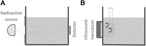
FIGURE 1. (A) Sketch of radiography setup. Radioactive source and detector are positioned opposite to each other with the mud layer between the two. Hence full penetration of the mud layer is required; (B) Sketch of ultrasonography setup. The ultrasound transducer is positioned on one side of the mud layer and acts as both a transmitter and a receiver. The emitted radiation is reflected or backscattered back to the transducer.

Visualization with radiography is based on a difference in absorption of the radiation. When particles in the fluid absorb more radiation compared to the surrounding fluid, they will appear as shadows on the image. As a consequence, full propagation of the radiation through the mud layer is required. Visualization using ultrasonography is based on the difference in acoustic impedance of particles compared to that of the fluid. When encountering a change in acoustic impedance the transmitted ultrasound waves will be reflected by the insonified particles. These reflection signals are recorded back by the transducer and represented as a function of brightness on the screen. The stronger the echo signal the brighter the reflecting particle will appear on the screen. Hence, full penetration of the mud layer is no longer required, allowing limitation of the propagation path of the waves and consequently loss of intensity. An initial more detailed evaluation of these two possible techniques involves determining the attenuation of the transmitted energy by mud. The physics of attenuation for both can be expressed with the Beer-Lambert law (Eq. 1). It shows that a medium attenuates the incoming radiation as a function of the attenuation coefficient and the propagation path length of the radiation through the medium. The loss of radiation intensity due to attenuation is expressed as the ratio of the intensity of incoming radiation to the intensity of outgoing radiation, further referred to as the transmission ratio. The determination of the transmission ratio allows to assess whether or not the radiation intensity emitted by available radiation sources are sufficient. Therefore, the attenuation coefficient of the mud and the required minimum intensity of the outgoing radiation must be specified.

$T=\frac{I_l}{I_0}=e^{\left(-\mu .l\right)}(1)$

Where T is the transmission ratio [-], I₀ is the incoming radiation intensity [W·m⁻²], I_l is the outgoing radiation intensity [W·m⁻²], μ is the attenuation coefficient of the radiated medium [m⁻¹] and l is the thickness of the radiated medium [m].

The attenuation coefficient is however different for each type of radiation. In case of electromagnetic waves, the attenuation coefficients of different media are more or less stable and can therefore be retrieved from extensive databases as a function of the photon energy level. Attenuation coefficients for ultrasound are less clear-cut. As mentioned by Ginzel and Turnbull (2016), the values of attenuation coefficients can already vary due to variations in material processing. Consequently, values of ultrasound attenuation coefficients of materials available in the literature cannot simply be used. It is therefore recommended that attenuation coefficients for ultrasound are determined experimentally for each case.

2.1 Radiography

As full propagation of the radiation through the mud layer is required (Figure 1A), further assessment of radiography will mainly focus on the amount of radiation able to propagate through the mud layer. First the total loss in radiation energy caused by the setup and the mud layer will be estimated allowing the assessment of various radiation sources differing in emitted energy levels and amount of radiation.

When a point source is used, which is common for radiography, one should take into account that the size of particles will be magnified on the image depending on the distances between the source, particle and detector (Figure 2). Magnification however needs to be limited to preserve the quality of the images and to avoid particles getting overshadowed by particles in front. The magnification limit is determined by the distance between source and particle (x₁) and the distance between particle and detector (x₂). While the latter is fixed as the thickness of the mud layer, the chosen magnification limit will determine the distance x₁.

FIGURE 2

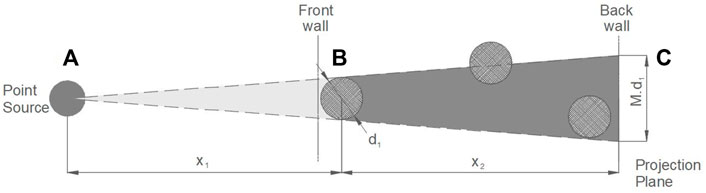
FIGURE 2. Principle sketch of the magnification of a projection by using a point source. The sketch shows the projection of a particle of size d₁ (B), present at the front, onto the projection plane of the detector at the back (C). The size of the projection is a factor M larger than the original particle size d₁. This magnification factor M is determined by the distance between the point source (A) and the particle (B), denoted by x₁, and the distance between the particle (B) and the projection plane on the detector (C), denoted by x₂. The larger the magnification factor M, the larger the shadow behind the particle, the more other particles are overshadowed and no longer visible on the projection.

As the magnification factor M [-] is inversely proportional to the distance between the radiation source and the mud particle x₁ [m] (Figure 2), limitation of the magnification factor will lead to an increase of x₁. While on the other hand x₁ should be kept to a minimum to limit energy loss, as the irradiance degrades by the distance squared (Eq. 2).

$D_{\mathit{rate}}\propto \frac{A}{d^2}(2)$

Where D_rate is the dose rate [Gy] at a distance d from the radiation source [m] and A is the activity of the radiation source [Bq]. For this evaluation the mud layer thickness is set to 560 mm, corresponding to an available test facility at Flanders Hydraulics Research (FHR). Limiting the magnification factor for the particles in the front to 1.56 results in a distance between the radiation source and the mud layer of 1 m, which is common in radiography.

To create adequate images for diagnostic use, a minimal dose rate absorbed by the detector is required. Although probably on the conservative side, the minimal dose rate for medical diagnostic imaging is used for this evaluation. Medical applications are always subject to the ALARA principle, which is an acronym for “As Low As Reasonably Achievable”. Hence it is an indication of the minimum dose rate required to create images of sufficient quality for diagnostic use. Recommendations on minimal dose rates for multiple medical applications are presented in IEC 62220-1-3:2008 (2008). Although the application on mud is not directly bound by a maximum dose rate, estimations show that these minimum dose rates are already hard to achieve for the intended ranges of flow speed and mud layer thickness. Therefore the highest dose rate recommended for medical applications of 2 μGy/frame is used for the continuation of this assessment.

Knowing the required dose rate at the detector allows to calculate the required intensity at the source if the loss in intensity due to propagation through mud is known. Such loss is caused by the attenuation capacity of mud, which comprises both absorption and scattering of the incoming waves. At higher energy levels, such as for x- and gamma radiation, intensity loss due to scattering becomes more significant and therefore cannot be neglected. Such intensity loss can be calculated using the Beer-Lambert law (Mayerhöfer et al., 2020), presented earlier as Eq. 1.

2.1.1 Attenuation of electromagnetic waves by mud

The attenuation coefficient of common materials or mixtures can be found in the literature. However, usually published is the mass attenuation, which is defined as:

${\mu }_{\mathit{mass}}=\frac{\mu }{{\rho }_{\mathit{mass}}}(3)$

Where μ_mass is the mass attenuation of the radiated medium [cm²·g⁻¹], μ is the attenuation coefficient of the radiated medium [cm⁻¹] and ρ_mass is the density of the radiated medium [g·cm⁻³]. Using the mass attenuation allows to express the attenuation as a function of density, which is convenient for media with changing density in time, like mud.

For this research the mass attenuation coefficients of the freely accessible database of the National Institute of Standards and Technology (NIST) are used (Berger et al., 2010). The NIST database contains a collection of published values of mass attenuation of chemical elements, compounds and common mixtures as a function of the energy level of the radiation, expressed in [MeV]. Unfortunately, the composition of mud varies according to its origin (port, river, area, etc.) and thus cannot be generalized. Therefore, the attenuation coefficient of each mud with different composition should be calculated. This can be done according to the method described in Ripan et al. (2016), using the values of mass attenuation of each compound (oxide) present in the mud in accordance with their weight fractions.

By means of a chemical element analysis using the Inductive Coupled Plasma—Optical Emission Spectrometry technique (ICP—OES, Wang (2004)), the different compounds present in mud were first determined together with their weight fractions for three mud densities: 1.035 g·cm⁻³, 1.100 g·cm⁻³ and 1.200 g·cm⁻³ (Table 1).

TABLE 1

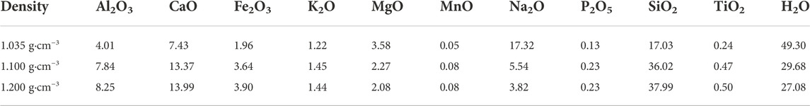
TABLE 1. Compounds present in mud originating from the Port of Zeebrugge (Begium) together with their respective weight fractions [%] as a function of mud density.

The mass attenuation values of these compounds can be found in the NIST database. With these data, the value of mass attenuation of the mud mixture can be calculated using the so-called “mixture rule”, presented in Burcu and Salih (2014) and shown as Eq. 4. This was done for each of the three previously mentioned mud densities used in this research. The resulting values of mass attenuation per density are plotted as a function of photon energy in Figure 3.

${\left(\frac{\mu }{\rho }\right)}_{\mathit{mix}}=\sum _{i=1}^N{\omega }_i.{\left(\frac{\mu }{\rho }\right)}_i(4)$

FIGURE 3

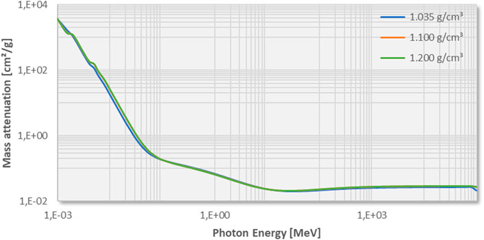
FIGURE 3. Mass attenuation coefficient as a function of photon energy level for multiple mud densities. Calculations are made using (Eq. 4), based on the weight fractions presented in Table 1 and mass attenuation coefficients found in the NIST database (Berger et al., 2010) for each of the compounds present in mud.

Where μ is the attenuation coefficient [cm⁻¹], ρ is the density [g·cm⁻³], ω is the weight fraction [%] and i is the reference to the elements in the mixture.

At first it can be concluded that the attenuation of mud is hardly influenced by the density. This is consistent with observations during consolidation experiments conducted FHR, presented in Meshkati Shahmirzadi et al. (2015); Pirola Igoa et al. (2020). For these experiments mud is pumped in large transparent columns and left at rest to settle and consolidate (see Supplemental Data, Supplementary Figure S1). Due to sedimentation a distinct interface between “clear” water and mud appears after some time (minutes to hours), which will settle with time (Berlamont et al., 1993). During such consolidation experiments, the settlement of this interface is recorded. Plotting the level of this interface as a function of time yields a characteristic settling curve. To accentuate this water-mud interface, Meshkati Shahmirzadi et al. (2015); Pirola Igoa et al. (2020) installed bright light panels behind the columns as shown in Supplemental Data, Supplementary Figure S1). This image of ongoing mud consolidation experiments shows that despite the lower density at the top of the mud layers, the mud-water interfaces are always clear and no light to dark shading can be seen with the depth of the mud column. These observations indicate the high opacity of mud regardless of mud density. Calculating the transmission coefficients as a function of radiation energy level, using the Beer-Lambert law (Eq. 1), confirms the opacity of mud for optical light (Figure 4). From the results it can be seen that even for mud layers of 1 mm thickness, a transmission ratio of minimal significance will be obtained with at least photon energy levels of 10 keV. This corresponds with low energetic X-rays which are still far more energetic compared to optical light (2–3 eV). Further focus is therefore on the use of high energy electromagnetic waves such as X-rays and gamma rays.

FIGURE 4

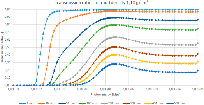
FIGURE 4. Transmission ratios calculated using eq. 1 and attenuation coefficients presented in Figure 3 (mud density 1.10 g·cm⁻³) and mud layer thickness ranging from 1 mm to 560 mm in a setup as depicted in Figure 1A.

2.1.2 Gamma rays

The electromagnetic spectrum shows that gamma rays have a higher energy level and therefore have a greater penetration capacity compared to X-rays. Hence it is reasonable to assume that with the use of gamma rays greater radiation doses are absorbed by the detector after full transmission through the mud layer. Gamma rays are produced by radioactive nuclei. After a radioactive nucleus undergoes alpha or beta radiation, the nucleus is left in an “excited” state. The nucleus then loses the excess energy by emitting a gamma photon. As a consequence the radiation emitted by a gamma source is typically mono-energetic. A broad variety of gamma ray sources are available on the market for different usage ranging from medical use to use in industrial processes. Common isotopes for industrial use are ⁶⁰Co and ¹³⁷Cs. Specifications of sources available on the market with these isotopes can be found in Supplementary Table S1 of the Supplemental Data (VEGA Americas, Inc, 2017).

Knowing the properties of the gamma source together with the attenuation coefficient of mud (corresponding to the photon energy level of the isotope) and the chosen magnification limit, the expected dose rate at the detector can be calculated as stipulated in Cember and Johnson (2008) or using the freeware Rad Pro Calculator McGinnis (2009). Results for a ¹³⁷Cs—185 GBq source are presented in Supplemental Data Supplementary Table S2. Using the minimum required radiation dose at the detector (ref. Section 2.1 Radiography) the maximum flow velocity can be determined as a function of the mud layer thickness. Defining a particle displacement limit between two consecutive frames, the maximum flow velocity can be deduced for varying mud layer thickness (Figure 5). A flowchart summarizing the complete calculation procedure is presented as Supplementary Figure S2 in the Supplemental Data.

FIGURE 5

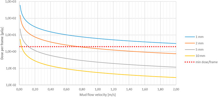
FIGURE 5. Radiation dose, originating from a ¹³⁷Cs–185 GBq source, received by the detector (Figure 1A) during the time span allowed for per image frame. The time span is expressed as mud flow velocity, where a maximum mud particle displacement of 5 mm is allowed for between two consecutive frames. Increasing mud flow velocity decreases the radiation time span for each image frame, hence the dose received per image frame. Curves for different mud layer thicknesses varying from 1 mm to 10 mm are presented. The dotted red line indicates the minimum dose required per image frame for adequate image quality.

These results (Figure 5) lead to the conclusion that with flow velocities up to 2 m·s⁻¹, the required dose rates at the detector can only be achieved for very thin mud layers of 1 mm–2 mm, which are mostly irrelevant for fluid dynamics applications. Despite the higher energy level, hence penetration capacity, the results with the ⁶⁰Co radiation source are even worse due to the lower activity of the source. This illustrates the importance of the activity over the photon energy level, making the use of X-rays more appropriate since activity rates of X-ray sources are much larger compared to the those of gamma ray sources.

2.1.3 X-rays

X-rays can be produced using an electric device like an X-ray tube. When electrical current is applied to it, X-rays are generated. While radiation from ⁶⁰Co and ¹³⁷Cs radioisotopes is mono-energetic, X-ray generators generate a spectrum of photon energy levels. As the attenuation coefficients of also determined by the energy level of the incoming radiation, the calculation of the transmission ratio of the radiation produced by an X-ray generator needs to be integrated over the fully generated energy spectrum. This makes the calculation of dose rates complex and requires the use of specially developed software. For this research, the “SpekCalc” software is used which is developed as a tool for medical research and educational applications [Poludniowski and Evans (2007); Poludniowski (2007); Poludniowski et al. (2009)].

Based on the voltage range of the X-ray source, the source angle and the distance between the X-ray source and the radiated object or patient, SpekCalc calculates the generated X-ray spectrum of the source and the dose rate received by the radiated object or patient. In practice a filter is usually placed between the source and the radiated object or patient. A well chosen filter (thickness and material) filters out the part of the generated photon energy spectrum which is not of interest or use. When passed through the filter the radiation is focused, so to speak. Therefore, a filter can also be taken into account in the SpekCalc software. The list of materials which can be chosen as filters is limited to a number of commonly used materials for X-ray filters, such as (Be, Al, Cu, Sn, W, Ta, H₂0, Ti and C). A combination of different filter materials is possible and the filter thickness is unrestricted.

The setup when applied in a hydraulic test facility with a source, mud layer and a detector (Figure 1A) is similar to the setup of a medical application with a source, filter and the patient. The detector at the back of the flume (Figure 1A) acts as the patient while the mud layer acts as the filter. With SpekCalc the radiation reaching the patient, or in this case detector, can be calculated while taking into account the attenuation due to the filter, in this case the mud layer. If SpekCalc is therefore used to estimate the dose rate behind the mud layer, the filter should be replaced by the mud layer. SpekCalc’s ability to set an arbitrary filter thickness allows to simulate the filter capacity of the mud layer. For any standard filter material available in the SpekCalc software, a thickness can be found such that it has the same attenuation value as the mud layer over a part of the energy spectrum. When selecting aluminum as filter material, the ratio of attenuation of the aluminum filter over the attenuation of mud with density 1.20 g·cm⁻³ is more or less constant over the entire energy spectrum of interest (Table 2). It can therefore be concluded that, with regards to the attenuation of X-rays over a photon energy spectrum of 10–400 keV, an aluminum filter with thickness of 26.69 cm is the equivalent of a 56 cm mud layer.

TABLE 2

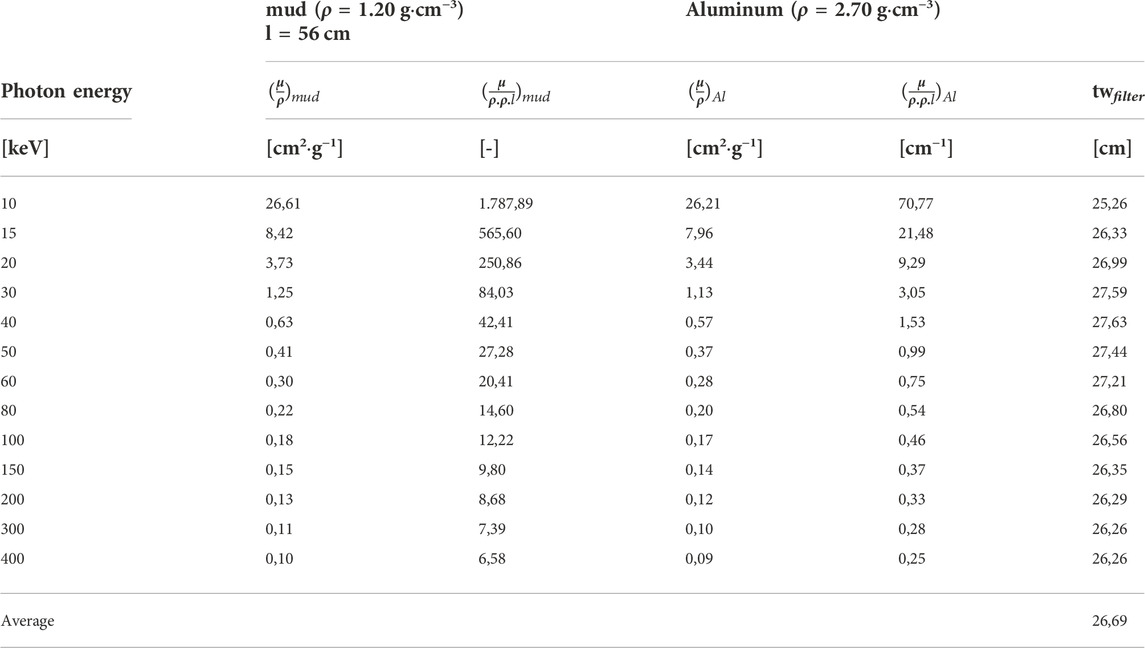
TABLE 2. Overview of required aluminum filter thickness for equivalent attenuation of a 56 cm thick mud layer with density 1.20 g·cm⁻³, as a function of photon energy. Calculated mass attenuation values of mud presented in Figure 3 were used to determine the attenuation values of the mud layer. Mass attenuation values of aluminum as from the NIST database (Berger et al., 2010) were used to determine the attenuation values of the aluminum filter.

It must be noted that the convenience of a constant ratio over a wide energy spectrum like presented in Table 2 does not hold true for all filter materials. Other filter materials only show a more or less constant ratio over a limited part of the spectrum. Copper for instance shows a more or less constant ratio over a limited spectrum from 10 to 40 keV, while for Beryllium this is from 150 keV to 400 keV. In case no constant ratio can be found over the entire energy spectrum, the spectrum needs to be split in parts. For each part of the spectrum a different equivalent filter material is then to be applied.

SpekCalc was originally developed for educational purposes, but meanwhile used in the medical community for first estimations of the expected dose rate. It is mostly referred to as “a commonly used analytical approximation” (Forth et al., 2017) and compared frequently in literature with other more advanced (Monte Carlo) code and/or measurements like in Poludniowski et al. (2009) and Forth et al. (2017). SpekCalc can therefore be considered as a reliable tool for first estimations of the dose rate. Forth et al. (2017) mentions overestimation of 10% and underestimation up to 20% by SpekCalc, compared to other simulations and validation measurements.

Nonetheless, a validation of the outcome of SpekCalc with actual measurements was also performed, if only to verify the software is properly used and the output correctly interpreted. The measurements were performed using an X-ray source allowing a voltage up to 250 kV, fitted with a Beryllium window of 3 mm and a Copper filter of 2 mm. The electric current applied on the tube was 2 mA and the dose rates were measured at a distance of 2 m. These dose rates are compared to the dose rates calculated using SpekCalc (Table 3).

TABLE 3

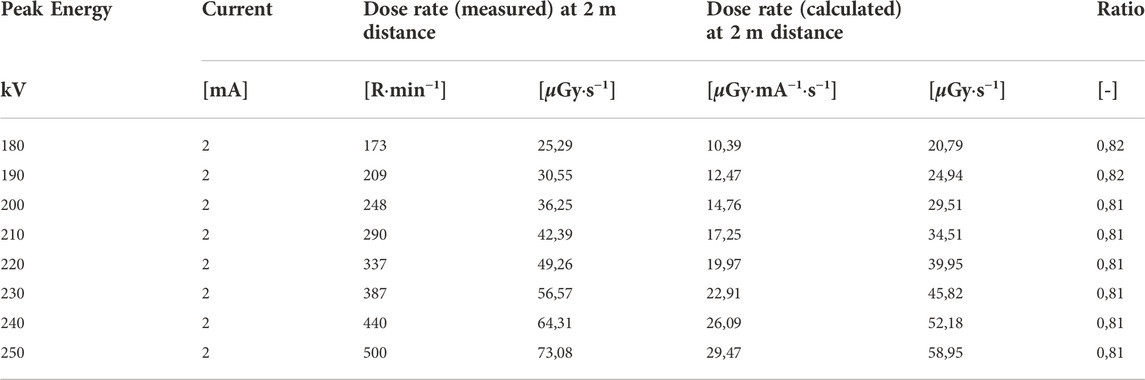
TABLE 3. Comparison of measured dose rates with calculated dose rates using SpekCalc software. Results show an underestimation of the calculated dose rate of 18–19%, which corresponds with the conclusions mentioned in Forth et al. (2017).

The results of the evaluation of the use of gamma sources imply that probably the more powerful X-ray generators are required for the intended application in mud. Therefore available X-ray generators used in the Non-Destructive Testing (NDT) industry were evaluated as they are less limited in power compared to generators for medical use. At first an X-ray generator with a high voltage range of 5—225 kV and a maximum current of 30 mA is considered. A schematic overview of the calculation procedure is presented as Supplementary Figure S3 in the Supplemental Data and the results in (Figure 6).

FIGURE 6

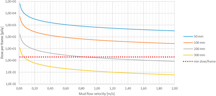
FIGURE 6. Radiation dose, originating from an X-ray 225 kV - 30 mA generator at max power, received by the detector (Figure 1A) during the time span allowed for per image frame. The time span is expressed as mud flow velocity, where a maximum mud particle displacement of 5 mm is allowed for between two consecutive frames. Increasing mud flow velocity decreases the radiation time span for each image frame, hence the dose received per image frame. Curves for different mud layer thicknesses varying from 50 mm to 300 mm are presented. The dotted red line indicates the minimum dose required per image frame for adequate image quality.

These results (Figure 6) confirm the importance of source activity prevailing over the photon energy level, as the considered X-ray generator shows the ability to visualize flows of 2 m·s⁻¹ over significantly thicker mud layers up to 200 mm. Nonetheless 200 mm is still insufficient for the intended hydraulic test facility supporting the nautical bottom research (ref. Section 2.1 Radiography). The most powerful “freely” available X-ray sources in the NDT industry have a voltage capacity up to 450 kV and a maximum current of 30 mA. Because of its medical background, SpekCalc is however limited to a maximum voltage of 300 kV. By means of interpolation expected results for X-ray generators exceeding 300 kV can still be estimated. Doing so for 450 kV generators set at 30 mA, shows they are up to 33 times more powerful compared to a generator with a voltage capacity of 225 kV. Nonetheless, multiplying the dose rate at the detector by 33 the maximum mud layer thickness still remains too limited with 300 mm.

2.2 Ultrasonography

Although ultrasonography does not require full transmission of the ultrasound radiation through the mud layer (ref. Section 2 Potential flow visualization techniques in mud), knowledge of acoustic properties of mud are also required to allow estimation of the maximum depth to which images of adequate quality can still be produced. Other research related to the acoustic properties of mud, like Pierce et al. (2015), mention however the lack of any available and trustworthy data. Measurements to determine the acoustic properties of mud are therefore required to fully evaluate the potential of ultrasonography.

2.2.1 Ultrasound properties of mud

In the Port of Zeebrugge a device called the Admodus USP pro is used to measure the density of the mud layers using ultrasound (Claeys et al., 2012; Plancke et al., 2018). The density of mud is determined by measuring the speed of sound through mud and the acoustic impedance of mud, where density is the product of the two. In addition, the Admodus USP pro also measures the attenuation of mud over a frequency spectrum of 1.0 MHz–3.5 MHz. From the data of a survey campaign performed in February 2019 in the Port of Zeebrugge (Meire et al. (2021)), these acoustic properties were retrieved as a function of mud density ranging from 1.00 g·cm⁻³ to 1.30 g·cm⁻³. The speed of sound through mud shows small variation in this density spectrum, from 1,460 m·s⁻¹ to 1,485 m·s⁻¹. Consequently, so does the acoustic impedance, ranging from 1,500 kg·m⁻²·s⁻¹ to 1900 kg·m⁻²·s⁻¹. The measured attenuation values range over a wider spectrum as they are function of both mud density and ultrasound frequency (Figure 7).

FIGURE 7

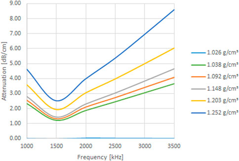
FIGURE 7. Attenuation values α_(f) of mud, as a function of ultrasound frequency and mud density. Values measured in Port of Zeebrugge using the Admodus USP pro [Meire et al. (2021)].

Despite the knowledge of these values for attenuation and speed of sound, evaluation whether or not the use of ultrasound waves would allow for sufficient penetration and energy conservation to create images of adequate quality for the application of a velocimetry algorithm is still not possible. Like for all medical applications, an optimal compromise between penetration depth, field of view and the different types of resolution (axial, lateral and time) will need to be determined (Alexander and Swanevelder (2011)). Nonetheless, the fact that the speed of sound and attenuation of human tissue and organs as specified in Hendee and Ritenour (2002), are in the same order of magnitude as the aforementioned values for mud, gives confidence that such a compromise can be found within the limits of standard acoustic medical equipment for depths similar to those for medical applications ranging from 5 cm to 15 cm.

2.2.2 Ultrasound brightness scan of mud

An ultrasound brightness scan, or B-scan, is the most familiar mode of ultrasound imaging for medical purposes. Probably the best known example is a fetal scan during a pregnancy. The images are typically grayscale, where the brightness of a pixel is a measure for the amplitude of the reflected signal at the corresponding position in the insonified area. Therefore strong reflectors such as muscle tissue will appear bright, while fluids will appear dark. In order to see any distinction in an image created with a B-scan some variety in acoustic impedance, which causes reflection, is thus required. To evaluate whether or not mud complies with this requirement the results of the chemical element analysis can be re-used (Table 1), providing the different oxides present in mud. For some of these oxides, the acoustic impedance can be found in literature. While the strength of a reflected signal is determined by the reflection coefficient, the reflection coefficient in turn is related to the difference in acoustic impedance encountered during propagation (Eq. 5).

$r_{ij}=\frac{Z_i-Z_j}{Z_i+Z_j}(5)$

Where r is the reflection coefficient [-], Z is the acoustic impedance [kg.m⁻²·s⁻¹] and i and j are the indices referring to the encountered materials or media. Acoustic properties found in literature should always be used carefully as such values are very variable contingent upon the origin of the medium [Ginzel and Turnbull (2016)]. Acoustic impedance found for Al₂O₃, SiO₂ and H₂O show however a great variety in value (respectively 37.9 kg·m⁻²·s⁻¹, 13.2 kg·m⁻²·s⁻¹ and 1.5 kg·m⁻²·s⁻¹ (Capilla et al., 2012; Sikorski, 2019)), while these oxides represent 74% weight percentage of mud with density 1.10 g·cm⁻³ (Table 1). This allows for the conclusion that significant reflections can be expected when an ultrasound wave is propagating through mud.

In wave physics there are different degrees of reflection depending on the ratio of the wavelength to the size of the reflecting object. While specular reflections are created by reflection on large objects, objects equal or smaller in size than the wavelength of the incident sound wave, will scatter the wave omni-directionally, resulting in much weaker reflection signals. The frequency range for this application is expected to be similar to those for medical imaging, ranging from 1 MHz to 10 MHz. With a speed of sound through mud of 1,460 m·s⁻¹ this results in wavelengths ranging from respectively 1,460 μm–146 μm. While the particle size distribution of mud in the Port of Zeebrugge, determined using a Mastersizer 2000 [Malvern Instruments Ltd. (2007)], shows a range of particle sizes ranging from 0.3 μm to 120 μm and a D50 around 6.5 μm. The results are presented in Supplementary Figure S4 of the Supplemental Data. It can thus be concluded that the reflecting particles in mud will always be smaller compared to the applied ultrasound wavelengths. Insonification of mud within the aforementioned ultrasound frequency range will therefore always result in scattering of the ultrasound waves.

In turn there are also different scattering regimes with different characteristics. Which regime is applicable is again determined by the ratio of scatterer size over wavelength. Scatterers smaller in size compared to the wavelength of the incident soundwave, as expected for the intended application, act as isotropic scatterers. This scattering regime is referred to as diffusive or Rayleigh scattering. In case of a high concentration of isotropic scatterers, a speckle-like signal will be created, as the scattered signals of each isotropic scatterer will reach the transducer over slightly different path lengths. This results in a so-called “Speckle Pattern” (Poelma, 2016), which in medical applications is typically created when scanning muscle tissue. This ratio between the size of the scatterer and the wavelength is expressed with the factor k. a where a is the radius of the scatterer [m] and k the wavenumber [m⁻¹], solely determined by the wavelength (Eq. 6).

$k=\frac{2.\pi }{\lambda }(6)$

Where λ is the wavelength of the ultrasound wave [m]. According to Szabo (2004), diffusive scattering occurs when k. a ⩽ 0.35. A lower limit is not mentioned. As scattering is a major contributor to the attenuation of sound waves, a lower bound for k. a must exist. In this case the scattered intensity becomes that small it is unable to reach back to the transducer before completely muted. With the determined particle size distribution of mud (Supplemental Data, Supplementary Figure S4), the diffusive scattering regime is therefore expected to be applicable when ultrasound frequencies of 1 MHz–10 MHz are used.

A small-scale test was performed at Ghent University Hospital, using a GE Vivid 7 ultrasound scanner equipped with a 10L linear array. For protection against the seawater present in mud, the array was inserted in a medical latex glove injected with acoustic gel to ensure good transmission of the ultrasound waves. This assembly was placed in a bucket of mud with a density of approximately 1.13 g·cm⁻³ (Figure 8). A B-scan of the mud was conducted with the ultrasound frequency set at 7 MHz.

FIGURE 8

FIGURE 8. Setup of performed B-scan on mud: (1) bucket of mud with density 1.13 g·cm⁻³, (2) 10L linear ultrasound array protected in a latex glove, (3) GE Vivid 7 ultrasound scanner. Apart from the array being immersed partly in the mud, the setup is in line with Figure 1B.

The resulting image (Figure 9) confirms the expectation of a speckle pattern image due to diffusive scattering of the ultrasound waves. As elaborated by Szabo (2004), a speckle pattern arises from the constructive and destructive interference of a great amount of scatterers, which appears as a light and dark mottled grainy pattern. For many years users of ultrasound systems assigned a diagnostic value to the appearance of speckle and assumed it was tissue microstructure. Despite its deceiving appearance as a tissue texture speckle is however an illusion and an unwanted effect for medical imaging as it reduces both image contrast as the distinction of subtle gradations and boundaries in tissue structure. Nonetheless, there are also medical applications which make use of the created speckle patterns, such as the monitoring of muscle tissue movement (cardiology) or the recording blood flows. This technique is referred to as “speckle tracking” by Garcia et al. (2018).

FIGURE 9

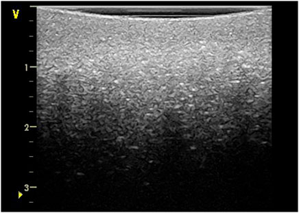
FIGURE 9. B-scan of mud with a ultrasound frequency set at 7 MHz, resulting in a clear speckle pattern due to interference scattered signals. Depth scale expressed in cm.

3 Whole flow-field velocimetry techniques

In experimental fluid dynamics optical PIV is currently widely used to measure flow velocities (Raffel et al., 2007). Despite the availability of many other techniques such as hot wire anemometers, pitot tubes, electromagnetic sensors, acoustic velocimeters or other intrusive flow measurement probes. The advantage of optical PIV is that it does not require intrusive probing and consequently does not cause distortion of the fluid flow. In addition, optical PIV allows for the evaluation of an entire 2D or even 3D flow field, enhancing the efficiency and quality of laboratory experiments. Therefore, by seeking alternative techniques to visualize the dynamics in mud, the intent of this research is to preserve these benefits of whole flow-field velocimetry techniques like optical PIV, while working in mud.

Optical PIV emerged from the earlier development of the (laser) speckle velocimetry (Garcia et al., 2018) and is based on the scattering of a laser’s light waves on particles seeded to the fluid, enabling visualization of the particles with an optical camera. The difference with the original speckle velocimetry is the scattering regime. Optical PIV acts in the Mie scattering regime, resulting in visualization of particles and not the interferences of multiple scattered waves, resulting in speckle patterns (Garcia et al., 2018). Adaptation of the optical PIV technique to be used with ultrasound imaging was conducted by Bohs and Trahey (1991) with the objective to obtain velocity vector fields in the blood circulation and strain imaging (muscle tissue movement). Because of far larger wavelengths of ultrasound waves used for ultrasound imaging, scattering of the ultrasound waves acts in the Rayleigh scattering regime, making it a resurgence of speckle velocimetry. When speckle velocimetry is applied to contrast-enhanced blood images (by addition of micro bubble particles) the technique is generally called “Echo PIV”, while when scattering is caused by scatterers present in the insonified tissue the technique is referred to as “speckle tracking” (Garcia et al., 2018).

Pursuant to the aforementioned elaboration of radiography and ultrasonography applied on mud, PIV can be applied on the images generated with radiography, while speckle tracking can be used on the images generated with ultrasonography.

3.1 Particle image velocimetry on radiographic images

Although radiography is deemed to be insufficient for the required mud thickness and flow velocities for nautical research, for other applications radiography may still be an option. To evaluate its potential use, an X-ray scan of a mud sample was conducted. The result of this scan is shown as Figure 10. The image shows that without the addition of contrast agents (e.g., the air bubbles which can be seen on the image as black dots), an X-ray scan of mud results in a homogeneous grayscale image, unsuited for the application of tracking algorithms. The black dots, originating from entrapped air bubbles, do can be used to be tracked. The air bubbles are the result of unwanted disturbance of the sample prior to the scan. However, due to their upward movement air bubbles influence the consolidation process, hence the behavior of mud. Therefore, when studying the dynamics in mud layer, the presence of air bubbles should be avoided. Thus, despite their suitability for tracking, the use of air bubbles cannot be considered in mud.

FIGURE 10

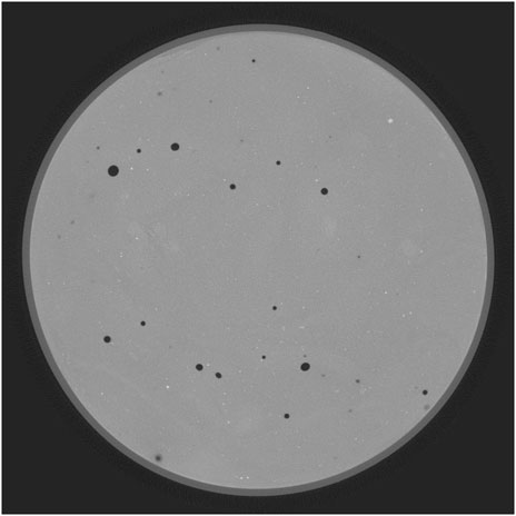
FIGURE 10. X-ray scan of mud. Apart from the black spots, the grayscale image is homogeneous. The black spots originate from entrapped air bubbles after disturbance of the sample.

Seeding the mud with tracing particles like in a conventional experimental setup for PIV recording (Raffel et al., 2007) is also not preferred. Ideally the particles added to the fluid are neutrally buoyant, ensuring their movement is solely caused by the flows in the fluid. In case of mud the density however changes over time, making it impossible to guarantee this aspiration, and undermining the credibility of the measurements. Furthermore, Manning and Whitehouse (2009) has shown that a change in sand fraction present in mud influences the flocculation and consolidation process of the mud. Because it is reasonable to assume that the presence of seeding particles will have a similar influence on the mud as sand particles, it can be questioned whether or not seeded mud still represents the mud of interest. For applications where these conditions do not apply [e.g., measurement of rheological parameters using a rheometer (Claeys et al., 2015)], flow velocity measurements can be performed using radiography and PIV.

3.2 Speckle tracking on ultrasonographic images

The aforementioned small-scale test using a standard medical ultrasound scanner on mud (Figures 8, 9) showed that the addition of seeding particles is uncalled for. Mud already contains a sufficient amount of small reflectors (scatterers) resulting in speckle pattern images suitable for the application of velocimetry algorithms, such as speckle tracking. To put this to the test a flow was induced in the mud bucket by moving a kitchen spoon back and forth. The spoon was at sufficient depth ($>$ 3 cm) below the array to ensure it was out of reach of the ultrasound waves (Figure 9). With the use of the speckle tracking application the scanner was able to record these induced flows as depicted in the 2 screenshots of the scanner (Figure 11), where the ensuing velocity vectors are plotted in a color scale in front of the B-mode speckle images. The blue and red colored vectors indicate similar flow velocities with opposite sign corresponding to the induced flows.

FIGURE 11

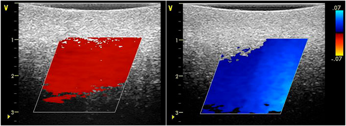
FIGURE 11. Screenshots during recording of induced flows with speckle tracking application. Depth scale in cm. Velocity scale in m·s⁻¹.

Unlike for medical applications, visualization of flows in mud does not require a clear distinction between different tissues or revealing tissue boundaries. Minimal requirements on lateral resolution are therefore not required, which allows to lower the ultrasound frequency (Alexander and Swanevelder (2011)) in order to increase the penetration depth. Lowering the frequency however lowers the wavenumber k (Eq. 6), while there will be a minimum value for the factor k.a as from where the scattering intensity becomes too low to be of any further use. Assuming the scatterers can be considered as rigid spheres, Szabo (2004) presents Eq. 7 for the Rayleigh scattering regime, showing the great influence of the ultrasound frequency (4^th power) and the scatterer radius (6^th power) on the scattering intensity. This shows the requirement to find a new compromise between penetration depth and ultrasound frequency while considering the minimal scattering intensity as an additional restriction. Because of the origin of speckle, the speckle quality is also dependent on the amount of scatterers present. As the latter is impossible to determine this new compromise will need to be determined experimentally.

$\frac{I_s}{I_i}=\frac{k^4.a^6}{9.r^2}.\left[1-\frac{3.\mathit{cos}\varphi }{2}\right](7)$

Where I_s is the scattering intensity [W·m⁻²], I_i is the incoming intensity [W·m⁻²], k is the wavenumber [m⁻¹], a is the scatterer radius [m], r is the distance to the scatterer [m] and ϕ the scattering angle [rad].

The relation between the scattering angle ϕ and the scattering intensity I_s might also allow for alternative setups. Eq. 7 shows the bi-polar scattering pattern with maximal intensities at ϕ = 0 (forward scattering) and ϕ = π (backscattering). For medical applications this is of course an advantage as it allows the use and flexibility of only one transducer while preserving maximal efficiency. For a stationary setup this flexibility is however of no use, while working in an angle by means of a second transducer is perfectly feasible (Figure 12). In such a setup one transducer would be used as a transmitter and the other transducer as the receiver. Compared to a setup with one transducer switching continuously between the two (Figure 1B) a setup with two transducers would allow for an increase in frame rate. In addition, working in an angle can allow optimization of the propagation path, decreasing the required penetration depth or even allow for evaluation of a 3D flow field. According to Eq. 7, the intensity will decrease with a factor 6.25 when working in an angle ϕ = π/2. Such a decrease in intensity can be compensated with an increase in frequency, e.g., 1 MHz–1.58 MHz. This will however lead again to higher attenuation, hence a decrease in penetration depth. Knowing the attenuation values of mud over the entire frequency range of interest will therefore be of great use to in order to evaluate whether or not the benefits of working in an angle are worth the decrease in penetration depth.

FIGURE 12

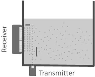
FIGURE 12. Sketch of an alternative setup for ultrasonography using two transducers, one as transmitter and a second as receiver.

4 Conclusion

This paper presents the evaluation methods and results for the application of known visualization techniques on mud. Because of some essential resemblances inspiration was found in the medical sector (ref. Section 2 Potential flow visualization techniques in mud), resulting in the selection of radiography and ultrasonography.

Review of the application of radiography on mud showed however that the technique is not efficient enough to be used in typically larger hydraulic research facilities. Even with the use of the most powerful radiation sources available on the market, either the mud layer thickness or the flow velocity should be limited in such a way that they are no longer relevant for the intended hydraulic research. Furthermore, the requirement to seed the mud with tracing particles to enable the application of PIV was demonstrated. Seeding with particles is however likely to influence the behavior of mud, making the reliability of the results questionable. In addition, the costs (direct and indirect) for the use of such radiation sources (above 100 kEUR) probably exceed most available budgets for hydraulic research projects. Nonetheless there are still applications (e.g. measurement of rheological parameters) for which these drawbacks might not apply and radiography together with PIV can be used.

As ultrasonography does not require full penetration of the mud layer. The focus to evaluate this technique is on finding a compromise between the penetration depth, frame rate and image quality. With a small-scale test it was shown that a common medical ultrasound scan of mud results in a so-called “speckle pattern”. Although speckle patterns are an unwanted feature for medical diagnostics, they are also used to track tissue movement or blood flow, known as “speckle tracking”. With the same small-scale setup speckle tracking was applied while inducing flows in the mud, demonstrating its ability to record and visualize the induced flows and determine flow velocities. Furthermore, the stationary deployment on hydraulic test facilities might provide the opportunity for alternative setups of ultrasound equipment, allowing to optimize its efficiency or even 3D flow field evaluation. Further customization of ultrasonography for application on mud in hydraulic test facilities will require the determination of attenuation values over a wide frequency range. Such data is however currently unavailable and therefore needs to be determined experimentally.

Data availability statement

Additional data is provided in the article/Supplementary Material, further inquiries can be directed to the corresponding author.

Author contributions

BB conducted the study and experiments and wrote the article. DM, JvB, and EL provided critical feedback and helped shape the research, analysis and manuscript.

Funding

This research is promoted by Flanders Hydraulics Research (FHR) and supported by the Maritime Technology Division of Ghent University in collaboration with the von Karman Institute for Fluid Dynamics (VKI). The joint research project of Maritime Technology Division, FHR and KU Leuven (Sotelo et al., 2022) is the incentive of this research.

Acknowledgments

The author is grateful to these institutions for the opportunity to conduct this research.

Conflict of interest

The authors declare that the research was conducted in the absence of any commercial or financial relationships that could be construed as a potential conflict of interest.

Publisher’s note

All claims expressed in this article are solely those of the authors and do not necessarily represent those of their affiliated organizations, or those of the publisher, the editors and the reviewers. Any product that may be evaluated in this article, or claim that may be made by its manufacturer, is not guaranteed or endorsed by the publisher.

Supplementary material

The Supplementary Material for this article can be found online at: https://www.frontiersin.org/articles/10.3389/feart.2022.878102/full#supplementary-material

References

Alexander, N., and Swanevelder, J. (2011). Resolution in ultrasound imaging. Continuing Educ. Anaesth. Crit. Care & Pain 11, 186–192. doi:10.1093/bjaceaccp/mkr030

CrossRef Full Text | Google Scholar

Berger, M. J., Hubbell, J. H., Seltzer, S. M., Chang, J., Coursey, J. S., Sukumar, R., et al. (2010). Xcom: Photon cross sections database. Gaithersburg, MD: National Institute of Standards and Instruments, Physical Measurement Laboratory, Radiation Physics Division.

Google Scholar

Berlamont, J., Ockenden, M., Toorman, E., and Winterwerp, J. (1993). The characterisation of cohesive sediment properties. Coast. Eng. 21, 105–128. doi:10.1016/0378-3839(93)90047-C

CrossRef Full Text | Google Scholar

Bohs, L. N., and Trahey, G. E. (1991). A novel method for angle independent ultrasonic imaging of blood flow and tissue motion. IEEE Trans. Biomed. Eng. 38, 280–286. doi:10.1109/10.133210

PubMed Abstract | CrossRef Full Text | Google Scholar

Burcu, A., and Salih, Z. E. (2014). The mass attenuation coefficients, electronic, atomic, and molecular cross sections, effective atomic numbers, and electron densities for compounds of some biomedically important elements at 59.5 kev. Sci. Technol. Nucl. Installations 2014, 8. doi:10.1155/2014/901465

CrossRef Full Text | Google Scholar

Capilla, J., Olivares, J., Clement, M., Sangrador, J., Iborra, E., and Devos, A. (2012). High-acoustic-impedance tantalum oxide layers for insulating acoustic reflectors. IEEE Trans. Ultrasonics, Ferroelectr. Freq. Control 59, 366–372. doi:10.1109/tuffc.2012.2205

PubMed Abstract | CrossRef Full Text | Google Scholar

Cember, H., and Johnson, T. E. (2008). “Radiation safety guides,” in Introduction to health physics. Fourth edition (New York City, NY: McGraw-Hill Education).

Google Scholar

Claeys, S., Dierikx, B., Paul, S., and Reenen, J. (2012). “Fluid mud density determination in navigational channels,” in Hydro12 - taking care of the sea. Rotterdam, Netherlands: Hydrographic Society Benelux. doi:10.3990/2.228

CrossRef Full Text | Google Scholar

Claeys, S., Staelens, P., Vanlede, J., Heredia, M., Van Hoestenberghe, T., Van Oyen, T., et al. (2015). “A rheological lab measurement protocol for cohesive sediment,” in Proceedings of INTERCOH2015: 13th international conference on cohesive sediment Transport processes. Editor E. Toorman (Leuven, Belgium: VLIZ Special Publication), 74, 20–21.

Google Scholar

de Wit, P. (1995). Liquefaction of cohesive sediments caused by waves. Delft: University Press.

Google Scholar

Delefortrie, G., and Vantorre, M. (2009). Prediction of the forces acting on container carriers in muddy navigation areas using a fluidization parameter. J. Mar. Sci. Technol. 14, 51–68. doi:10.1007/s00773-009-0041-x

CrossRef Full Text | Google Scholar

Delefortrie, G., and Vantorre, M. (2016). Ship manoeuvring behaviour in muddy navigation areas : State of the art. Hamburg, Germany: Bundesanstalt für Wasserbau, 26–36. doi:10.18451/978-3-939230-38-0_4

CrossRef Full Text | Google Scholar

Delefortrie, G., Vantorre, M., Verzhbitskaya, E., and Seynaeve, K. (2007). Evaluation of safety of navigation in muddy areas through real-time maneuvering simulation. J. Waterw. Port Coast. Ocean Eng. - ASCE 133, 125–135.

CrossRef Full Text | Google Scholar

Forth, L., Speller, R., and Moss, R. (2017). “The importance of accurate x-ray energy spectra for modelling dose deposition with Monte Carlo techniques,” in IEEE nuclear science symposium and medical imaging conference (Atlanta, GA: NSS/MIC), 1–2. doi:10.1109/NSSMIC.2017.8533113

CrossRef Full Text | Google Scholar

Gao, Z., Yang, H., and Xie, M. (2015). Computation of flow around wigley hull in shallow water with muddy seabed. J. Coast. Res. 73, 490–495. doi:10.2112/SI73-086.1

CrossRef Full Text | Google Scholar

Garcia, D., Lantelme, P., and Saloux, E. (2018). “Chapter 26: Introduction to speckle tracking in cardiac ultrasound imaging,” in Handbook of speckle filtering and tracking in cardiovascular ultrasound imaging and video. London, United Kingdom: Institution of Engineering and Technology (IET). doi:10.1049/PBHE013E_ch26

CrossRef Full Text | Google Scholar

Ginzel, E., and Turnbull, B. (2016). Determining approximate acoustic properties of materials. e-Journal Nondestruct. Test. (NDT) 21 21 (12), 23–33. doi:10.1002/jgrc.20103

CrossRef Full Text | Google Scholar

Hendee, W. R., and Ritenour, E. R. (2002). “Ultrasound waves,” in Medical imaging physics (New York: Wiley-Liss). doi:10.1002/0471221155.ch19

CrossRef Full Text | Google Scholar

Hsu, W. Y., Hwung, H. H., Hsu, T. J., Torres-Freyermuth, A., and Yang, R. Y. (2013). An experimental and numerical investigation on wave-mud interactions. J. Geophys. Res. Oceans 118, 1126–1141. doi:10.1002/jgrc.20103

CrossRef Full Text | Google Scholar

IEC 62220-1-3:2008 (2008). Medical electrical equipment - characteristics of digital X-ray imaging devices - Part 1-3: Determination of the detective quantum efficiency - detectors used in dynamic imaging. Geneva, Switzerland: International Electrotechnical Commission.

Google Scholar

Kaidi, S., Lefrançois, E., and Smaoui, H. (2020). Numerical modelling of the muddy layer effect on ship’s resistance and squat. Ocean. Eng. 199, 106939. doi:10.1016/j.oceaneng.2020.106939

CrossRef Full Text | Google Scholar

Lovato, S., Keetels, G. H., Toxopeus, S. L., and Settels, J. W. (2022). An eddy-viscosity model for turbulent flows of herschel–bulkley fluids. J. Newt. Fluid Mech. 301, 104729. doi:10.1016/j.jnnfm.2021.104729

CrossRef Full Text | Google Scholar

Malvern Instruments Ltd. (2007). Mastersizer 2000 user manual (MAN0384-1.0). Worcestershire WR14 1XZ, United Kingdom: Author.

Google Scholar

Manning, A. J., and Whitehouse, R. J. S. (2009). “Uop mini-annular flume – operation and hydrodynamic calibration,” in HR Wallingford technical report, TR 169. London, United Kingdom: IntechOpen.

Google Scholar

Mayerhöfer, T., Pahlow, S., and Popp, J. (2020). The bouguer-beer-lambert law: Shining light on the obscure. Chem. Phys. Chem. 21, 2029–2046. doi:10.1002/cphc.202000743

CrossRef Full Text | Google Scholar

McGinnis, R. (2009). Rad pro calculator. Available at: http://www.radprocalculator.com/ (Accessed June, 2020).

Google Scholar

Meire, D., Claeys, S., De Maerschalck, B., and Mostaert, F. (2021). “Evaluatie van meetinstrumenten voor de bepaling van slib karakteristieken: Deelrapport 3: Meetcampagne februari 2019,” in Versie 5.0. WL rapporten, 18_059_3 (Antwerpen: Waterbouwkundig Laboratorium), 1–49.

Google Scholar

Meshkati Shahmirzadi, M. E., Staelens, P., Claeys, S., Cattrysse, H., Van Hoestenberghe, T., Van Oyen, T., et al. (2015). “Experimental investigation on consolidation behaviour of mud: Subreport 1- methodology study,” in Versie 5.0. WL rapporten, 12_082 (Antwerp: Flanders Hydraulics Research), 26.

Google Scholar

Pierce, A. D., Siegmann, W. L., and Brown, E. (2015). “Analytical discussion of past measurements of acoustic attenuation in mud sediments and of possible future experimental approaches,” in Proceedings of meetings on acoustics. Jacksonville, FL: Acoustical Society of America. doi:10.1121/2.0000221

CrossRef Full Text | Google Scholar

Pirola Igoa, E., Ibanez, M., Claeys, S., Meire, D., and Mostaert, F. (2020). “Experimental investigation on the consolidation behaviour of mud: Port of hamburg,” in Versie 3.0. FHR reports, 18_009_1 (Antwerp: Flanders Hydraulics Research), 42 + 17.

Google Scholar

Plancke, Y., Meire, D., and Mostaert, F. (2018). “Studie naar meettechnieken voor het onderzoeken van de opbouw van sliblagen in het deurganckdok: Deelrapport 1 – bundeling van de belangrijkste resultaten uit 3 masterproeven uitgevoerd op de universiteit antwerpen,” in Versie 3.0. WL rapporten, 12_160_1 (Antwerpen: Waterbouwkundig Laboratorium), 201–213.

Google Scholar

Poelma, C. (2016). Ultrasound imaging velocimetry: A review. Exp. Fluids 58, 3. doi:10.1007/s00348-016-2283-9

CrossRef Full Text | Google Scholar

Poludniowski, G. (2007). Calculation of x-ray spectra emerging from an x-ray tube. part ii. x-ray production and filtration in x-ray targets. Med. Phys. 34, 2175–2186. doi:10.1118/1.2734726

PubMed Abstract | CrossRef Full Text | Google Scholar

Poludniowski, G., and Evans, P. (2007). Calculation of x-ray spectra emerging from an x-ray tube. part i. electron penetration characteristics in x-ray targets. Med. Phys. 34, 2164–2174. doi:10.1118/1.2734725

PubMed Abstract | CrossRef Full Text | Google Scholar

Poludniowski, G., Landry, G., Deblois, F., Evans, P., and Verhaegen, F. (2009). Spekcalc: A program to calculate photon spectra from tungsten anode x-ray tubes. Phys. Med. Biol. 54. doi:10.1088/0031-9155/54/19/N01

PubMed Abstract | CrossRef Full Text | Google Scholar

Pouv, K. S., Besq, A., and Guillou, S. (2012). Rheometric study for elaborating transparent model cohesive sediments for local investigations of erosion behaviour. Rev. paralia 5, 1.1–1.14. doi:10.5150/revue-paralia.2012.001

CrossRef Full Text | Google Scholar

Pouv, K. S., Besq, A., Guillou, S., and Toorman, E. A. (2014). On the cohesive sediment erosion: A first experimental study of the local processes of transparent model materials. Adv. Water Resour. 72, 71–83. doi:10.1016/j.advwatres.2014.05.012

CrossRef Full Text | Google Scholar

Raffel, M., Willert, C., Wereley, S., and Kompenhans, J. (2007). Particle image velocimetry: A practical guide. 2nd edition. New York: Springer.

Google Scholar

Ripan, B., Hossain, S., Abdus, S. M., and H, M. F. (2016). Calculation of gamma-ray attenuation parameters for locally developed shielding material: Polyboron. J. Radiat. Res. Appl. Sci. 9, 26–34. doi:10.1016/j.jrras.2015.08.005

CrossRef Full Text | Google Scholar

Sikorski, W. (2019). Development of acoustic emission sensor optimized for partial discharge monitoring in power transformers. Sensors 19, 1865. doi:10.3390/s19081865

PubMed Abstract | CrossRef Full Text | Google Scholar

Soltanpour, M., Shamsnia, S. H., Shibayama, T., and Nakamura, R. (2018). A study on mud particle velocities and mass transport in wave-current-mud interaction. Appl. Ocean Res. 78, 267–280. doi:10.1016/j.apor.2018.06.019

CrossRef Full Text | Google Scholar

Sotelo, M. S., Boucetta, D., Doddugollu, P., Toorman, E., Brouwers, B., Van Hoydonck, W., et al. (2022). “Experimental study of a cylinder towed through natural mud,” in Proceedings of MASHCON 2022: 6th international conference - port manoeuvres (Ghent, Belgium: Ghent University). [Unpublished manuscript].

Google Scholar

Szabo, T. L. (2004). “Wave scattering and imaging,” in Diagnostic ultrasound imaging: Inside out (Elsevier Academic Press).

CrossRef Full Text | Google Scholar

Toorman, E., and Berlamont, J. (2015). “Fluid mud in waterways and harbours: An overview of fundamental and applied research at ku leuven,” in PIANC yearbook 2015 (Brussels, Belgium: PIANC), 211–218.

Google Scholar

Vanlede, J., Toorman, E., Liste Muñoz, M., Rocabado, I., Heredia, M., Delefortrie, G., et al. (2014). “Towards cfd as a tool to study ship-mud interactions,” in Oceanology international (Flanders Hydraulics Research). Poster.

Google Scholar

Vantorre, M. (1997). “Approach channels - a guide for design,” in Ptc 11-30: Final report of joint working group PIANC-IAPH II, in cooperation with IMPA and I ALA. Supplement to PIANC Bulletin no. 95 (Brussels, Belgium: PIANC), 108.

Google Scholar

VEGA Americas, Inc. (2017). Operating Instructions VEGASOURCE 35 Source holder. Schiltach, Germany: VEGA Grieshaber KG.

Google Scholar

Wang, T. (2004).“Inductively coupled plasma optical emission spectrometry” in Analytical instrumentation handbook. Third Edition, 57–74.

CrossRef Full Text | Google Scholar

Zaynab, T., Jarny, S., and Texier, A. (2015). “Rheology and local study of a transparent model cohesive sediment,” in INTERCOH2015: 13th international conference on cohesive sediment Transport processes. Editor E. A. Toorman (Leuven, Belgium: VLIZ Special Publication), 74, 7–11.

Google Scholar