Comprehensive Analysis for Long-Term Hydrological Simulation by Deep Learning Techniques and Remote Sensing

Xu, Chaowei; Wang, Yizhen; Fu, Hao; Yang, Jiashuai

doi:10.3389/feart.2022.875145

ORIGINAL RESEARCH article

Front. Earth Sci., 20 April 2022

Sec. Environmental Informatics and Remote Sensing

Volume 10 - 2022 | https://doi.org/10.3389/feart.2022.875145

This article is part of the Research Topic Research of Remote Sensing and Big data Convergence on Environmental Assessments View all 5 articles

Comprehensive Analysis for Long-Term Hydrological Simulation by Deep Learning Techniques and Remote Sensing

Chaowei Xu^†

Yizhen Wang^†

Hao Fu*

Jiashuai Yang

College of Urban and Environmental Sciences, Peking University, Beijing, China

Hydrological simulation plays a very important role in understanding the hydrological processes and is of great significance to flood forecasting and optimal allocation of water resources in the watershed. The development of deep learning techniques has brought new opportunities and methods for long-term hydrological simulation research at the watershed scale. Different from traditional hydrological models, the application of deep learning techniques in the hydrological field has greatly promoted the development trend of runoff prediction and provides a new paradigm for hydrological simulation. In this study, a CNN–LSTM model based on the convolutional neural network (CNN) and long short-term memory (LSTM) network, and a CNN–GRU model based on CNN and gated recurrent unit (GRN) are constructed to study the watershed hydrological processes. To compare the performance of deep learning techniques and the hydrological model, we also constructed the distributed hydrological model: Soil and Water Assessment Tool (SWAT) model based on remote sensing data. These models were applied to the Xixian Basin, and the promising results had been achieved, which verified the rationality of the method, with the majority of percent bias error (PBE) values ranging between 3.17 and 13.48, Nash–Sutcliffe efficiency (NSE) values ranging between 0.63 and 0.91, and Kling–Gupta efficiency (KGE) values ranging between 0.70 and 0.90 on a monthly scale. The results demonstrated their strong ability to learn complex hydrological processes. The results also indicated that the proposed deep learning models could provide the certain decision support for the water environment management at the watershed scale, which was of great significance to improve the hydrological disaster prediction ability and was conducive to the sustainable development of water resources.

1 Introduction

Hydrological simulation uses a mathematical model to simulate the hydrological process in the basin and realizes it on the computer, which is one of the most important tasks in hydrological research (Mishra et al., 2017; Koster et al., 2018; Qi, Zhang, and Wang 2019; Xu, Han, and Fu 2022). It has received extensive attention from hydrologists and has become an important tool for studying watershed water resources (Arsenault et al., 2015; Xiong et al., 2019; Zhou et al., 2019). Hydrological simulation also has a very important guiding significance for the sustainable utilization of water resources (Ravazzani et al., 2015; Wang G. Q. et al., 2015; Wang H. L. et al., 2015; Xu Y. Y et al., 2020; Yin Z. L et al., 2021).

At present, the main method of hydrological simulation at the watershed scale is the watershed hydrological model (Freeze and Harlan 1969; Bultot and Dupriez 1976; Beven and Kirkby 1979; Zhao 1992; Arnold et al., 1998; Edijatno et al., 1999). The watershed hydrological model is a scientific way that generalizes complex hydrological phenomena and processes to simulate the runoff generation and confluence of the watershed. The study of the watershed hydrological model provides us with an important tool for scientific understanding and rational utilization of water resources, and provides an important scientific basis for water resources management and decision-making (Fonseca et al., 2014). The watershed hydrological model includes a lumped model and distributed model, and also a semi-distributed model (Jaiswal, Ali, and Bharti 2020). The rapid development of remote sensing technology has provided a lot of convenience for the application of distributed hydrological models (Silvestro et al., 2015; Xu et al., 2021). The Soil and Water Assessment Tool (SWAT), designed and developed by Jeff Arnold in the 1990s for the U.S. Department of Agriculture (USDA) Agricultural Research Service (ARS) (Arnold et al., 1998; Srinivasan, Arnold, and Jones 1998), is a comprehensive watershed distributed hydrological model, which has an explicit physical mechanism. The SWAT model is designed to simulate the quality and quantity of surface and groundwater and predict the environmental impact of land use, land management practices, and climate change, which is widely applied over the world (Arnold et al., 2012; Fohrer et al., 2014; Dwarakish and Ganasri 2015; Krysanova and Srinivasan 2015; Worku, Khare, and Tripathi 2017; Nguyen and Dietrich 2018; Tan et al., 2019; Xue et al., 2019; Raihan et al., 2020). The SWAT model has a strong physical foundation, which can simulate a variety of hydrological physical and chemical processes, such as runoff and sediment by spatial information provided by remote sensing and GIS (Worku, Khare, and Tripathi 2017). SWAT has a global user community with an active technical support forum that facilitates its applications to be an effective tool for watershed management (Samimi et al., 2020).

In addition to the watershed hydrological model, deep learning techniques have also been widely used in the hydrological field due to their small data requirements and strong plasticity (Rezaeianzadeh et al., 2014; Beven 2020; Gu et al., 2020; Van et al., 2020). Especially in recent years, the explosive development of deep learning has brought innovations and breakthroughs to hydrological simulation and will become an important research direction in the future (Abbas et al., 2020; Alizadeh et al., 2021; Lei et al., 2021). It will also become an important driving force to promote the development of hydrological simulation of basins and provide new opportunities for the research and application of flood forecasting (Sit et al., 2020). Deep learning can effectively improve the summary and expression of data distribution rules with the increase in training samples and the diversification of data characteristics, thus improving the prediction accuracy of runoff and many hydrological simulation cases based on deep learning have emerged (Althoff, Rodrigues, and da Silva 2021; Bai H. et al., 2021; Hussain et al., 2020). The usage of deep learning in a previously published article can be seen in a related study (Sit et al., 2020). We can see that the commonly used deep learning networks for hydrological forecasting mainly include the long short-term memory network (LSTM) (Hochreiter and Schmidhuber 1997), convolutional neural network (CNN) (Lecun 1989), and gated recurrent unit (GRU) (Cho et al., 2014). LSTM is a widely used deep learning model, which can better deal with hydrological data with long-term dependence. It is very suitable for processing time series data such as hydrological and water quality information and has been successfully applied to the field of hydrological forecasting (Hu et al., 2019; Xu W. et al., 2020; Bai Y. et al., 2021; Feng et al., 2021; Lees et al., 2021; Lu et al., 2021; Yin H. L. et al., 2021; Yuan et al., 2021). The convolution layer and pooling layer of CNN can better mine the effective information contained in the data and retain the characteristics of the data in the time dimension, which is conducive to and improves the prediction accuracy of hydrology simulation (Pulido-Calvo and Portela 2007; Kabir et al., 2020; Kim and Song 2020; Van et al., 2020). GRU is further optimized on the basis of LSTM and gets a more concise expression. Studies have shown that GRU can achieve good performance in various hydrological prediction tasks (Ayzel and Heistermann 2021; Sibtain et al., 2021; Zhao et al., 2021).

However, related studies have shown that a single model has not yet been able to extract spatiotemporal features simultaneously, which affects the prediction accuracy in the hydrology field (Chhetri et al., 2020; Miau and Hung 2020). The combination of deep learning models can give full play to the advantages of each model and improve the generalization ability, thereby improving the performance of the model (Chhetri et al., 2020). The combination of CNN and LSTM can not only quickly extract the effective features in the data but also fully consider the long-term dependence of the time series, so as to achieve accurate runoff prediction, which has a certain reference value for mastering the hydrological environment of the basin (Hong et al., 2020). Similarly, combining the advantages of CNN’s spatial processing capability and GRU’s temporal processing capability can also be applied to hydrological forecasting (Miau and Hung 2020). Hence, in order to improve the simulation accuracy and increase the generalization ability, this study combines CNN with LSTM and GRU to construct the CNN–LSTM model and CNN–GRU model. Then the two deep learning models and the SWAT model are applied to hydrological simulation at a watershed scale with long-term hydrological data. The main objectives of this study are 1) to develop the coupled models: CNN–LSTM and CNN–GRU based on deep learning techniques; 2) to evaluate the performance of the proposed deep learning models against the existing hydrology model (SWAT model). The remainder of this article is organized as follows: Section 2 describes the methods and study area; Section 3 summarizes the research results; Section 4 is the discussions; and lastly, the conclusions are drawn in Section 5.

2 Materials and Methods

Deep Learning Models

CNN is a commonly used feedforward neural network in deep learning, which is mainly composed of five parts: input layer, convolution layer, pooling layer, dense layer, and output layer. The convolutional layer is the core of the CNN neural network, where convolution is performed when data are passed to the convolution layer.

The input layer is expressed by Eq. 1:

X = [\begin{matrix} x_{1,1} & \dots & x_{1, n} \\ ⋮ & \cdot & ⋮ \\ x_{m, 1} & \dots & x_{m, n} \end{matrix}], (1)

where $X$ represents the input data matrix, $x$ represents the data feature, $n$ represents the length of time, and $m$ is the number of data features.

The convolution layer is carried out by using Eq. 2 and the time series can be obtained through the convolution layer:

O_{c} = f_{c} (X \otimes W_{c} + b_{c}), (2)

where $\otimes$ is convolution operation, the convolution kernel $W_{c}$ is weight vector, $b_{c}$ is the bias, $f_{c} (\cdot)$ is activation function, ReLu usually, and $O_{c}$ is mapping results.

The pooling operation is used to select the most important features of the convolutional layer sequence. The commonly used pooling method is maximum pooling, which is expressed as Equation 3 and Equation 4:

O_{p} (k) = m a x (O_{c} (2 k - 1), O_{c} (2 k)), (3)

O_{p} = max (O_{c}), (4)

where $O_{p} (k)$ is the $k$ -th pooling result and $O_{p}$ is the global maximum pooling result.

Finally, the combination of temporal features is implemented by the dense layer, and the output layer outputs the results of the dense layer, as shown in Equation 5 and Equation 6.

O_{d} = f_{d} (O_{p} \times W_{d} + b_{d}), (5)

y = f_{o} (O_{d} \times W_{o} + b_{o}), (6)

where $W_{d}$ is the weight matrix of the dense layer, $b_{d}$ is bias, $f_{d} (\cdot)$ is the activation function of the dense layer, $W_{o}$ is the weight matrix of the output layer, $b_{o}$ is the bias of the output layer, and $f_{o}$ is the activation function of the output layer, Softmax usually.

LSTM is a variant structure of the recurrent neural network (RNN) and has three “gate” structures, namely the forget gate, input gate, and output gate, and a memory unit to selectively receive information transmitted into the neural network.

Forget gate:

f_{t} = σ (W_{f} \cdot [h_{t - 1}, x_{t}] + b_{f}), (7)

Input gate:

i_{t} = σ (W_{i} \cdot [h_{t - 1}, x_{t}] + b_{i}), (8)

Output gate:

o_{t} = σ (W_{o} \cdot [h_{t - 1}, x_{t}] + b_{o}), (9)

where $σ$ is Sigmoid function, $b_{f}$ , $b_{i}$ , $b_{c}$ , and $b_{o}$ are the corresponding bias; $W_{f}$ , $W_{i}$ , $W_{c}$ , and $W_{o}$ are the weight matrixes; $t a n h$ is hyperbolic tangent function; $h_{t - 1}$ is the output of hidden state of previous step; and $x_{t}$ is the input.

The GRU network is an improved network based on LSTM. GRU combines the forget gate and input gate into an “update gate.”

The calculation of the GRU unit neural network is as follows:

f_{t} = σ (W_{f} \cdot [h_{t - 1}, x_{t}]), (10)

i_{t} = σ (W_{i} \cdot [h_{t - 1}, x_{t}]), (11)

\tilde{h_{t}} = t a n h (W_{c} \cdot [f_{t} h_{t - 1}, x_{t}]), (12)

h_{t} = (1 - i_{t}) h_{t - 1} + i_{t} \tilde{h_{t}}, (13)

where $x_{t}$ is the input, $f_{t}$ is a reset gate, $i_{t}$ is an update gate, $t a n h$ is the activation function, $σ$ is the sigmoid function, $\tilde{h_{t}}$ is the hidden state, $h_{t}$ is the output of the hidden state, $h_{t - 1}$ is the output of the hidden state of the previous step, and $W_{f}, W_{i},$ and $W_{c}$ are the weight matrixes of the corresponding gate and the hidden state.

Because a single neural network often has limitations in dealing with practical problems, it is a development trend to combine two or more algorithms in order to make use of their respective advantages. Hydrological data has the characteristics of temporal and spatial correlation, so it is necessary to combine the advantages of each model for comprehensive modeling. With learning spatial (CNN) and temporal (LSTM) features, a new deep learning scheme was proposed in this study, called CNN–LSTM. The framework of the proposed CNN–LSTM model is outlined in Figure 1A and can be expressed as Eqs 14-16. In addition, we also constructed a CNN–GRU model to compare the performance of different combined models (Figure 1B).

C O = f (X \otimes W + b), (14)

where $X$ is the input matrix, $f$ is Relu function, $\otimes$ is the convolution operation, $W$ is the weight, and $b$ is the bias.

q_{t} = f ([\begin{matrix} q_{t, i} \\ e_{t, j} \\ r_{t, j} \end{matrix}]), (15)

q_{t, i} = q_{t - 1}, q_{t - 2}, \dots q_{t - i} e_{t, j} = e_{t - 1}, e_{t - 2}, \dots e_{t - j} r_{t, j} = r_{t - 1}, r_{t - 2}, \dots r_{t - j}, (16)

where $q_{t}$ is the prediction discharge at time t, $q_{t, i}$ is the discharge from the previous t-i to t-1 (i is the time scale), $e_{t, j}$ is the evaporation from the previous t-j to t-1 (j is the time scale), $r_{t, j}$ is the rainfall from the previous t-j to t-1, and $f (\cdot)$ is the system transfer function.

FIGURE 1

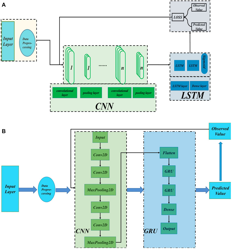
FIGURE 1. Flowchart of the proposed deep learning models (A) CNN–LSTM and (B) CNN–GRU.

Soil and Water Assessment Tool Model

The SWAT model is a continuous, physically based, and distributed hydrologic model. The SWAT model is widely used to simulate water quality and quantity as well as to assess the impacts of physical changes to a catchment, such as land use and climate changes. The hydrology module is the main module of the SWAT model, including surface runoff, infiltration, subsurface runoff, evapotranspiration, snowmelt runoff, and transmission loss. The hydrological process of the SWAT model is calculated in two parts: slope runoff and channel flood routing. The water balance equation is the calculation basis of water transfer in SWAT.

S W_{t} = S W_{0} + \sum_{i = 1}^{t} (R_{d a y} - Q_{s u r f} - E - W_{s e e p} - Q_{g w}), (17)

where $S W_{t}$ is the soil moisture content at termination time, $S W_{0}$ is the soil moisture content at start time, $R_{d a y}$ is rainfall, $Q_{s u r f}$ is the surface runoff, $E$ is evapotranspiration, $W_{s e e p}$ is the lateral flow, $Q_{g w}$ is the return flow of groundwater, all measured in mm, and $t$ is time, measured in months or days. The calculation of $Q_{s u r f}$ is crucial and can be expressed by a Soil Conservation Service Curve Number (SCS-CN) method (Division, United States. Soil Conservation Service. Engineering, 1986):

Q_{s u r f} = \frac{{(R_{i} - I_{a})}^{2}}{R_{i} - I_{a} - S}, R_{i} > I_{a}, (18)

S = \frac{25400}{CN} - 254, (19)

where $R_{i}$ is the precipitation, $I_{a}$ is the initial abstraction, and $S$ is the potential maximum retention after the beginning of the runoff. The CN is the parameter corresponding to various soil and land conditions and can be obtained from tables (Grove, Harbor, and Engel 1998). If $R_{i} < I_{a}$ , $Q_{s u r f} = 0$ .

The potential evapotranspiration is calculated using the Penman–Monteith method (Jung, Lee, and Moon 2016). A kinematic storage model is used to predict the lateral flow, whereas the return flow is simulated by creating a shallow aquifer (Arnold et al., 1998). The Muskingum method is used for channel flood routing (Mccarthy 1939).

When the model is built, the watershed is divided into several sub-basins according to the digital elevation model (DEM), and then the sub-basins are further divided into several hydrological response units (HRU) according to different land use and soil types. The SWAT model runs separately on each HRU unit to predict the runoff of each HRU, and then the total runoff of the watershed is obtained through channel flood routing.

Study Area and Dataset

The Xixian Basin is located in Xinyang city, in the southeast of Henan Province, with an area of 10,190 km² (31.52°–32.72° N, 113.25°–114.77° E) (Figure 2). The main rivers of the basin are the Shi River, ZhuGan River, and Qingshui River, which belong to the Huaihe River Basin. The terrain exhibits high elevation in the east and low elevation in the west, elevations in the study area range from 40 to 1,020 m, with a mean elevation of 142 m (Figure 2). The annual rainfall is 800–1400 mm, with a mean value of 1,060 mm, 50% takes place in the flood season (focused on June to September). The average potential evaporation is 850 mm. The Xixian Basin has a humid to semi-arid transition zone with a temperature of about 14–16°C. The major land-use types of the study area are forest and cultivated land.

FIGURE 2

FIGURE 2. Study area.

The hydrological data of the study are from the hydrological bureau, including rainfall, evaporation, and discharge data (monthly scale) from 1976 to 1997. The major geospatial input data include climate data, terrain map (Figure 2), soil data (Figure 3A), and land use/land cover map (Figure 3B). Spatial input data used to set up SWAT were sourced from publicly available datasets (Table 1). The accuracy of these datasets has been evaluated and widely used in hydrological simulations (Li et al., 2013; Fuka et al., 2014; Satge et al., 2015; Alemayehu, van Griensven, and Bauwens 2016; Zhao 2016; Alemayehu et al., 2018; Bouslihim et al., 2019; Duan et al., 2019; Rivas-Tabares et al., 2020).

FIGURE 3

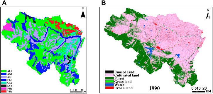
FIGURE 3. Geographic information of the study area: (A) soil types and (B) land use.

TABLE 1

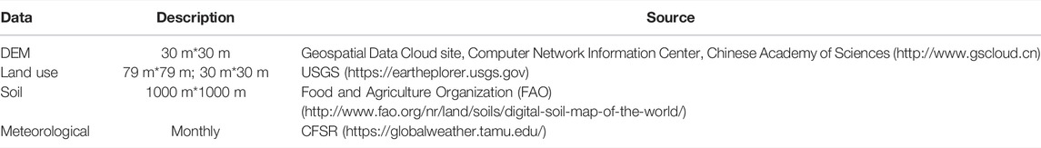
TABLE 1. Data source and description.

Model Setting

2.1.1 Soil and Water Assessment Tool Model Setting

The SWAT model for the Xixian Basin has been built using information concerning land use, soil properties, and climate data. ArcSWAT (2012 version) is used as the graphical user interface for the SWAT model. The SWAT model setup includes four steps: watershed delineation, hydrological response unit analysis, input database building, and SWAT simulation: 1) First, with the “Watershed automatic delimitation,” all the topographical inputs were calculated starting from a 30 m resolution DEM to define the watershed features like boundaries, river network, sub-basins, and to derive slope related parameters. 2) The second phase is the HRU definition. The land-use code is converted into a code that can be recognized by SWAT through the land-use index table. The soil data came from the Food and Agriculture Organization of the United Nations (FAO) (Table 1), which was reclassified into 8 categories, and then Soil-Plant-Air-Water (SPAW) software was used to calculate the attributes required by the SWAT soil database. The soil index table was also established. The land area in a sub-basin can be further divided into the HRUs, which are the basic computing elements of the SWAT model. In this study, a sub-basin was subdivided into only one HRU that was characterized by the dominant land use and soil type. 3) Third, “Write Input Table,” daily meteorological data, including temperature, relative humidity, sunshine duration, wind speed, and rainfall, were obtained from the databases of Climate Forecast System Reanalysis (CFSR: https://climatedataguide.ucar.edu/climate-data/climate-forecast-system-reanalysis-cfsr). Rainfall data came from hydrological stations in the watershed. These data were written to SWAT tables for SWAT simulation. 4) Fourth, “SWAT simulation,” set the name of the simulation, output, simulation period, and other information for simulation and then run the simulation. The parameter sensitivity analysis (200 model runs) was also performed with the auto-calibration software SWAT-CUP using the Sequential Uncertainty Fitting (SUFI2) optimization program for streamflow (Abbaspour, Vejdani, and Haghighat 2007). The p-value and t-stat are used to evaluate the sensitivity of the SWAT model parameters. The smaller the p-value, the larger the t-stat and the more sensitive it is. The results of parameters sensitivity analysis are shown in Figure 4. We can see that the curve number (CN) is the most sensitive parameter for streamflow simulation. The period 1975 to 1976 served as a warm-up period for the model, allowing state variables to assume realistic initial values for the calibration period. Monthly discharges from 1976 to 1990 are used for calibration and the remaining data from 1990 to 1997 are used to validate. The selected parameters are summarized in Table 2.

FIGURE 4

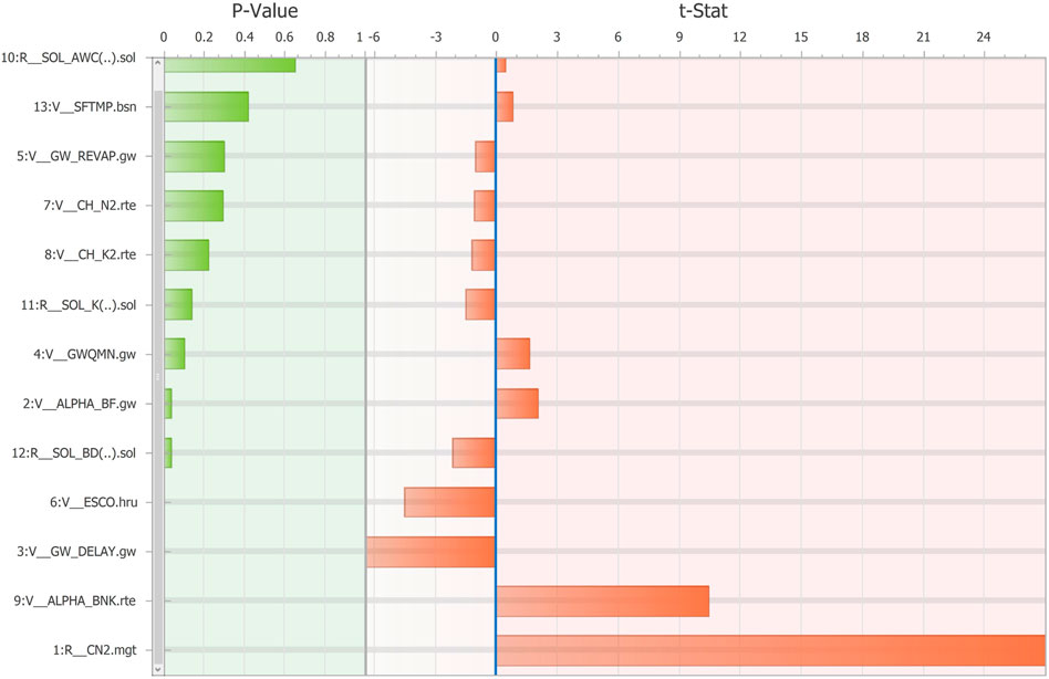
FIGURE 4. Results of parameter sensitivity analysis.

TABLE 2

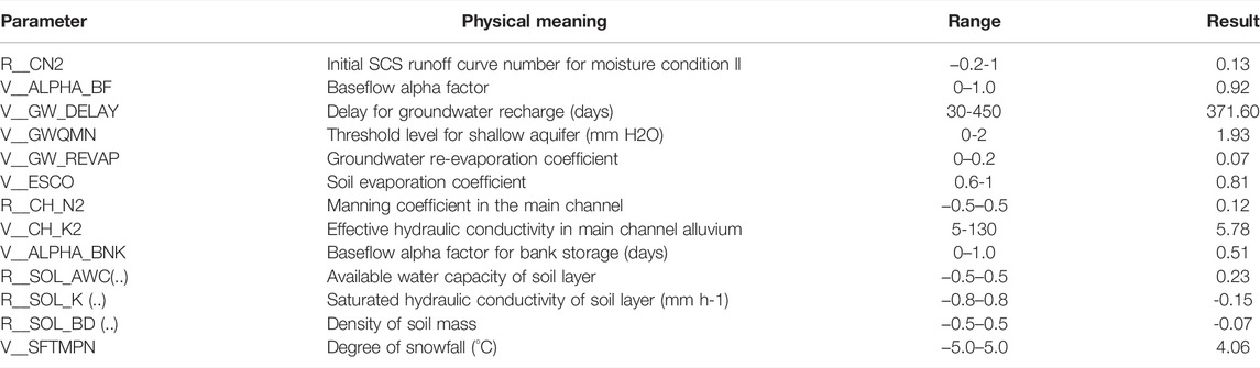
TABLE 2. Calibrated values of the model parameters.

2.1.2 Deep Learning Models Setting

This study constructs integrated deep learning models (CNN–LSTM and CNN–GRU) based on the MATLAB language. The CNN–LSTM model constructed in this study mainly includes the following steps (Figure 5): 1) the rainfall runoff and its related factors are pre-processed by a standardized method and the input characteristic map is obtained by sliding window. 2) Feature extraction is carried out for the characteristic map of runoff through CNN, in which the convolution layer and pool layer can compress the number of parameters, so as to extract more obvious features reflecting the change of streamflow and reduce overfitting and the dense layer can summarize and output the aforementioned features. 3) The extracted features are converted into the corresponding data format of LSTM through the LSTM layer. Through the three-gate mechanism in LSTM, the data mining of time series is carried out to obtain its internal change of streamflow and obtain the prediction model. 4) The sigmoid function is used as the output activation function to output the result of the prediction. The settings of the CNN–GRU model are similar. In all, normalized input (rainfall evaporation and streamflow) is passing to the CNN layer. The feature output (after the convolution layer) is input to LSTM/GRU by a flattening layer.

FIGURE 5

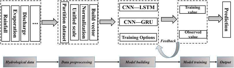
FIGURE 5. Technology roadmap of deep learning models for rainfall-runoff simulation and prediction.

The super parameter setting affects the performance of the models to a certain extent. Throughout all of our experiments, the relatively better super parameter and activation function are determined: first, a sequence input layer inputs sequence data to a network. The folding layer is used to convert sequences to a batch of images. Then, a 2D convolutional layer with 32 filters of size (10 1) and "same’ padding is used. After the normalization, we create an average pooling layer with pool size (1 1) and stride (10 10). The activation function is “elu.” Apply sequence unfolding layer and flatten layer to transform the input into channel dimensions, and then feed the features to two LSTM layers. The hidden units of each LSTM layer are 128 and 32, respectively. We also added a dropout layer to prevent the model from overfitting with a probability of 0.25. Finally, fully connected layer and regression layer are used to output. The Adam is chosen as the optimizer. In this study, we used the root mean square error (RMSE) as an objective criterion. The training process is shown in Figure 6.

FIGURE 6

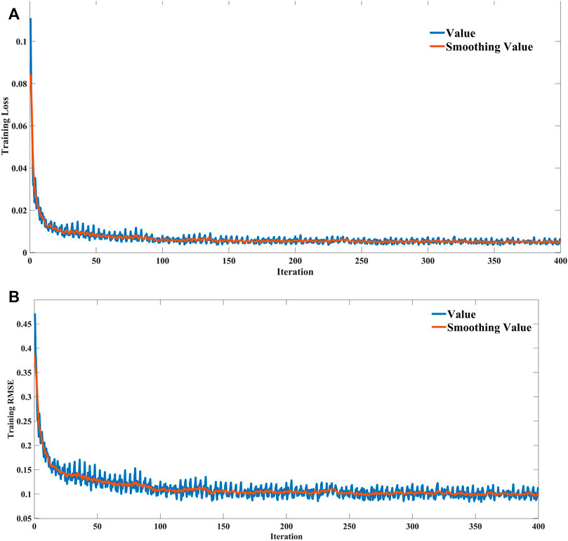
FIGURE 6. Train processes. (A) Training loss; (B) training RMSE).

Statistical Criteria and Model Evaluation Performance

The performance of the deep learning models and SWAT model can be computed using statistical indices and graphical comparisons. The Nash–Sutcliffe efficiency (NSE) (Legates and McCabe 1999), percent bias error (PBE) (Bennett et al., 2013), and Kling–Gupta Efficiency (KGE) (Gupta et al., 2009) were adopted to evaluate the model performance.

N S E = 1 - \frac{\sum {(Q_{o} - Q_{s})}^{2}}{\sum {(Q_{o} - \bar{Q_{o}})}^{2}}, (20)

P B E = \frac{\sum Q_{s} - \sum Q_{o}}{\sum Q_{o}} * 100 %, (21)

K G E = 1 - \sqrt{{(r - 1)}^{2} + {(α - 1)}^{2} + {(β - 1)}^{2}}, (22)

α = \frac{σ_{s}}{σ_{o}} β = \frac{\bar{Q_{s}}}{\bar{Q_{o}}}, (23)

where $Q_{o}$ is the observed discharge, $Q_{s}$ is the simulated discharge, $\bar{Q_{o}}$ is the mean of observed discharge, $\bar{Q_{s}}$ is the mean of simulated discharge, $σ_{s}$ is the standard deviation of simulated discharge, $σ_{o}$ is the standard deviation of observed discharge, and $r$ is the correlation coefficient.

3 Results

Land-Use Change

Due to data source limitations, we analyzed the land use in the basin from 1990 to 1997. The distribution of the land-use area ratio of Xixian watershed is shown in Figure 7. It can be seen that there are five types of land use in the study area, mainly including cultivated land and forest land, which account for about 90% of the basin area. Of these, cultivated land is the main land-use type, accounting for about 60% and the second is forest, accounting for about 30%. In order to fully demonstrate the degree of land type transfer of Xixian watershed from 1990 to 1997, the rates of change in land use were used to conduct the research. The rates of change of land used in the study area are shown in Table 3. It is worth noting that the degree of land-use change in the study area is not obvious, which is very beneficial for our research, and will have a litter impact on the hydrological model.

FIGURE 7

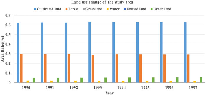
FIGURE 7. Distribution of land-use area ratio of Xixian watershed.

TABLE 3

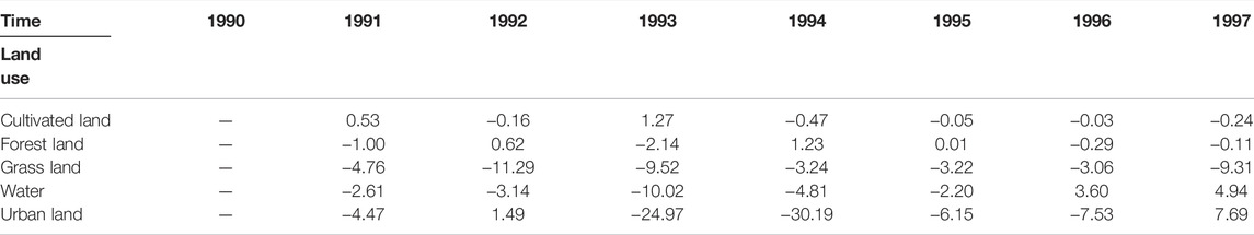
TABLE 3. Rates of change of land use of the study area from 1990 to 1997.

Comparing the Results of Deep Learning Models and Hydrological Model

The calibration results in Table 2 were input into the SWAT model. The results of the deep learning models were artificially divided into calibration and validation periods. The discharge hydrographs and the relationship between observed and simulated discharges are shown in Figure 8. The observed and simulated discharge agreed well (Figure 8A and Figure 8B), indicating both SWAT and deep learning models represented observed discharges well. All correlation coefficients (both calibration and validation period) were above 0.8, suggesting that both SWAT and deep learning models captured the study area’s hydrologic characteristics well and reproduced acceptable discharge simulations. However, the SWAT model has poor performance in the initial stage (Figure 8D), which is due to the watershed state at the initial time is not really enough. In addition, there was a significant difference between the calibration and validation period; both deep learning models and the SWAT model were well in the calibration period, while the SWAT model was better in the validation period (Table 4). This may be linked to the variability of rainfall and runoff. Deep learning models were less effective for time series simulation with greater variability, and the SWAT model was suitable for long-term prediction. Moreover, the performance was very similar for the two deep learning methods (Figures 8E,F), which was also consistent with the characteristics of deep learning. The PBE of deep learning models was less than 10% for both calibration and validation period, which revealed super fine simulation performance in the flood volume. This illustrated the advantages of deep learning in time series data processing. The PBE of the SWAT model was less than 20% but greater than 10% for validation periods and all PBE>0. The reason was that the overall physical mechanism of the SWAT model was clear and represented the entire hydrological process, so the overall fit was better (NSE is closer to 1). The deep learning models were the mining of hydrological data and have no physical meaning behind it, so it is better for the simulation of data values (the PBE is relatively small), but not as good as the SWAT model for the overall discharge hydrograph. In addition, we could find that the simulation result of the SWAT model was always greater than the observed value in low discharge, which was the reason why the PBE>0. KGE could integrate NSE and PBE to better evaluate the model performance. There is substantial variation in results across the calibration and validation period of deep learning models and SWAT model; deep learning performed well during calibration but SWAT during validation. This also verified the impact of data variability on deep learning models.

FIGURE 8

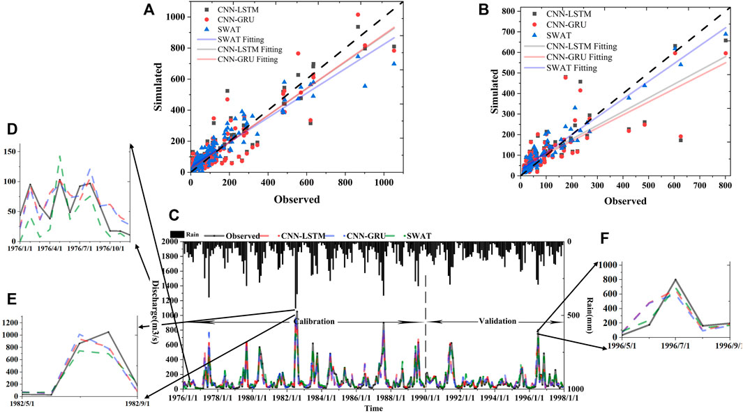
FIGURE 8. Simulated results of deep learning models and hydrological model (the scatters of different models in (A) calibration and (B) validation period; the discharges hydrographs in (C) 1976–1997, (D) 1976, (E) 1992, and (F) 1997 years).

TABLE 4

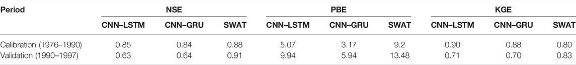
TABLE 4. Comparison of prediction performances in deep learning models and hydrological model.

Comparing the Deep Learning Results for Different Leading Times

To evaluate the simulation ability of the deep learning models in various leading times, 1-, 5-, and 10-month-ahead discharges were set. The discharge hydrographs and scatter diagrams are shown in Figure 9. In different leading times, the models had obtained satisfactory results, indicating that the relationship between rainfall and runoff in the basin was relatively stable, and it is less affected by anthropogenic activities. However, when the leading time is 1, the model performance of CNN–GRU was not as good as 5 and 10 (the scatter of the deviates from the ideal fit in Figure 9A) whereas there was a little difference in CNN–LSTM (Figure 9B), which indicated that the performance of the CNN–LSTM model is more stable. The CNN–LSTM model had better generalization capability and prediction accuracy. In summary, the deep learning model’s performance in different leading times indicated that deep learning techniques could provide an acceptable prediction precision.

FIGURE 9

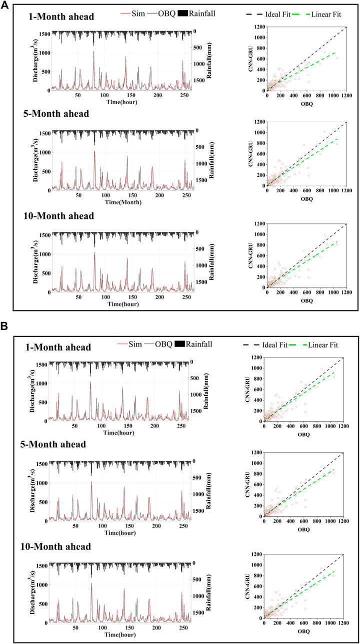
FIGURE 9. Predicted results and scatters of different leading times (A) CNN–GRU; (B) CNN–LSTM (OBQ: observed discharge; Sim: simulation discharge).

Size-Dependent of Training Samples in Deep Learning Models

In order to explore the influence of training samples on the simulation performance, the training set sizes of CNN–LSTM and CNN–GRU are set to 70%, 50, and 30% respectively, and other super parameters remain unchanged. We can see that when the training set becomes smaller, the model performance also decreases (Table 5). Therefore, although deep learning can obtain better results, there are certain requirements for the data set. In addition, compared with the CNN–LSTM model, the size of the training set has a greater impact on the CNN–GRU model (the red circle in Figure 10), indicating that the CNN–GRU model is more sensitive to the size of training samples, which may be related to the internal structure of CNN–GRU: GRU has a simpler structure, a gate less than LSTM, fewer parameters, and simplifies matrix operation, so the performance of GRU is more dependent on data set than LSTM. We also find that the training samples are not better (Table 5). Therefore, the selection of appropriate samples has a certain impact on the model results.

TABLE 5

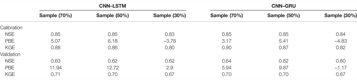
TABLE 5. Performance of deep learning models under different size of training samples.

FIGURE 10

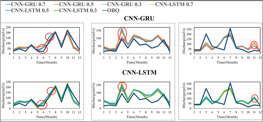
FIGURE 10. Results of deep learning modes under different training samples (in turn: 1981, 1992, and 1997).

4 Discussion

The land-use change has an important impact on runoff simulation (Cheng et al., 2022; Wang et al., 2021). However, the land-use change in the study area is small (Table 3), so the results of this study are not affected by the land-use change. From the results in sections 3.2–3.4, we can see that deep learning models acquire an acceptable predicted value but not as well as the SWAT model in some respects. This is because deep learning models do not consider the changes of heterogeneity within the basin, but only mine and extract information features from the data to find its rules for training and prediction, which leads to a higher level representation of the underlying data sources (Saba et al., 2019). Furthermore, deep learning is capable of extracting substantial features without being explicitly instructed, hence, it is more immune to raw and noisy data (Sahiner et al., 2019); however, it cannot consider the variability of rainfall and runoff caused by anthropogenic activities. The SWAT model needs to calibrate parameters through certain underlying surface data, meteorological data, and hydrological data to comprehend the model (Arnold et al., 1998), hence, it considers more variables. It can also be seen from Figure 10 that all models have a good simulation effect in large discharge, but the simulation error is large in low discharge. This verifies that the change in the underlying surface has a greater impact on small floods in the basin and the model is more suitable for simulating the flow of large floods (Breuer et al., 2009). We can also see that the SWAT model has poor performance in the initial stage (Figure 10D), which may be related to the data or the setting of the watershed state at the initial time, which is also the reason why the SWAT model is not as accurate as deep learning models in the initiation stage. Therefore, physical models, though are deterministic and reliable, do not always perform well due to their intrinsic limitations (Islam 2011).

Although the deep learning models have achieved well results, they cannot show the internal process of runoff simulation, have no practical physical significance, and cannot be carried out through certain measurements or remote sensing data (Isik et al., 2013). Moreover, the deep learning models have a certain dependence on training samples and the scale of training samples has an important impact on the effect of deep learning models (section 3.4). If a flood event is beyond the training data range, the model would perform poorly with high uncertainty. The SWAT model can apply in the ungauged watershed with related remote sensing data (Sisay et al., 2017). In addition, the SWAT model is based on the physical process and its mechanism is independent of the size of training samples. It can simulate the runoff at any point of the river in the basin and completely simulate the process from rainfall to runoff in all sub-basins. Therefore, the simulation space of the SWAT model is wider. The SWAT model can also explore the impact of climate change or human activities (under different land-use environments) on runoff change (Swain et al., 2021).

In all, it is notable that the deep learning models can be applied to the hydrological simulation at a monthly scale and the results are good (Table 4 and Figure 8). However, several studies have shown that deep learning has certain requirements for datasets: the distribution curve of datasets should be smooth (Gong et al., 2014; Jaderberg et al., 2015). For data with abnormal points, especially mutation points and low correlation, the deep learning models will have certain problems or special processing of abnormal data (Cubuk et al., 2018; Feng et al., 2020; Irrgang et al., 2020; Zuo et al., 2020). This research studies the hydrological simulation on the monthly scale, which meets the specific requirements of the deep learning model for the input data. For the continuous hydrological simulation on the daily scale or the hourly scale, because the data show mutation points, corresponding processing operations need to be carried out, which also needs to be further studied in the future. However, the deep learning models do not need too much watershed information but only need hydrological data, which are more convenient to apply. Hence, it is necessary to select an appropriate model according to the comprehensive balance of application and data requirements in the future.

5 Conclusion

This study develops the deep learning models, and the distributed hydrological model for hydrological simulation and the results show their applicability. The proposed architecture builds the foundation for subsequent hydrological analysis. This study mainly has the following conclusions: 1) the time series neural network: CNN–LSTM and CNN–GRU are constructed and applied to simulate the monthly discharge in Xixian Basin. At the same time, the distributed hydrological model—SWAT model—is compared and analyzed. 2) The model’s application ability is evaluated in the Xixian Basin. The results demonstrate that both models can provide a good performance at basin-scale hydrological simulation. 3) Although deep learning techniques can be used for hydrological simulation, their training set and leading times have a certain impact on the simulation results, and reasonable model settings should be carried out to obtain the optimal solution. 4) The CNN network is used to extract local features of data, and LSTM and GRU networks are used to learn and predict time series to realize deep mining of data features. Their combination solves the problem that a single model is difficult to obtain the optimal solution, and provides new ideas and methods for hydrological simulation to improve the accuracy of flood volume.

Data Availability Statement

The original contributions presented in the study are included in the article/Supplementary Material, further inquiries can be directed to the corresponding author.

Author Contributions

Conceptualization, CX and YW; Data curation, CX; Formal analysis, CX and YW; Investigation, HF; Methodology, CX and YW; Project administration, HF; Resources, HF; Software and code, CX and YW; Supervision, HF; Writing—original draft, CX and YW; Writing review & editing, YW and JY.

Funding

This research was funded by the Major Science and Technology Program for Water Pollution Control and Treatment (Grant No. 2014ZX07203-008).

Conflict of Interest

The authors declare that the research was conducted in the absence of any commercial or financial relationships that could be construed as a potential conflict of interest.

Publisher’s Note

All claims expressed in this article are solely those of the authors and do not necessarily represent those of their affiliated organizations, or those of the publisher, the editors, and the reviewers. Any product that may be evaluated in this article, or claim that may be made by its manufacturer, is not guaranteed or endorsed by the publisher.

References

Abbas, A., Baek, S., Kim, M., Ligaray, M., Ribolzi, O., Silvera, N., et al. (2020). 'Surface and Sub-surface Flow Estimation at High Temporal Resolution Using Deep Neural Networks. J. Hydrol. 590. doi:10.1016/j.jhydrol.2020.125370