 Andreas Wagner
 Benjamin Fersch
 Peng Yuan
 Thomas Rummler2†
 Harald Kunstmann
- 1Institute of Meteorology and Climate Research (IMK-IFU), Karlsruhe Institute of Technology (KIT), Garmisch-Partenkirchen, Germany
- 2Institute of Geography, University of Augsburg, Augsburg, Germany
- 3Geodetic Institute (GIK), Karlsruhe Institute of Technology (KIT), Karlsruhe, Germany
The assimilation of observations in limited area models (LAMs) allows to find the best possible estimate of a region’s meteorological state. Water vapor is a crucial constituent in terms of cloud and precipitation formation. Its highly variable nature in space and time is often insufficiently represented in models. This study investigates the improvement of simulated water vapor content within the Weather Research and Forecasting model (WRF) in every season by assimilating temperature, relative humidity, and surface pressure obtained from climate stations, as well as geodetically derived Zenith Total Delay (ZTD) and precipitable water vapor (PWV) data from global navigation satellite system (GNSS) ground stations. In four case studies we analyze the results of high-resolution convection-resolving WRF simulations (2.1 km) between 2016 and 2018 each in every season for a 650 × 670 km domain in the tri-border-area Germany, France and Switzerland. The impact of 3D VAR assimilation of different variables and combinations thereof, background error option, as well as the temporal and spatial resolution of assimilation is evaluated. Both column values and profiles derived from radiosondes are addressed. Best outcome was achieved when assimilating ZTD and synoptic data at an hourly resolution and a spatial thinning distance of 10 km. It is concluded that the careful selection of assimilation options can additionally improve simulation results in every season. Clear effects of assimilation on the water budgets can also be seen.
Introduction
The careful selection of the model system, forcing data or model options and settings contribute to high-quality simulation results in limited area models (LAMs). But also convection permitting models with state-of-the-art model-physics, which have undergone a thorough model setup (Prein et al., 2015; Wagner et al., 2018), are not necessarily a true reflection of reality. Lorenz (1965) claimed early that simulation quality strongly depends on the initial state of a model. Thus, data assimilation, which is the procedure of optimizing the initial state (Daley, 1991; Navon, 2009; Guerova et al., 2016) may contribute to improve simulation results. Especially tropospheric water vapor with a highly variable nature in space and temporal variations that can reach more than 50% within a few hours (Johasson et al., 1998) places high demands on model performance. Water vapor is a crucial constituent in terms of cloud and precipitation formation, so special attention is required also to its vertical distribution. Thus, remote sensing data, providing profiles or column values of water vapor information are promising candidates for assimilation into LAMs. Improvement by the assimilation of Interferometric Synthetic Aperture Radar (InSAR) data was demonstrated for weak and moderate precipitation (Pichelli et al., 2014) and also for other hydrometeors (Mateus et al., 2016). The history of assimilation of Global Navigation Satellite System (GNSS) microwave signals goes back to the early 1990’s (Bevis et al., 1992). Different products are currently utilized. Profiles from radio occultation, i.e., a remote sensing technique used for measuring the physical properties of a planetary atmosphere from the GNSS, are operationally assimilated by weather services, such as the Met Office, Météo France, European Centre for Medium-Range Weather Forecasts (ECMWF) and the German Weather Service (DWD), to reduce biases of temperature, wind and humidity in their operational and reanalysis models (Poli et al., 2008; Rennie, 2010; Anlauf et al., 2011). Studies assimilating Precipitable Water Vapor (PWV) and Zenith Total Delay (ZTD) derived from GNSS data are the most common. Rohm et al. (2019) and Giannaros et al. (2020) presented recent results assimilating GNSS data in the WRF model. A positive or neutral impact on the forecast of rain amount, rain location and humidity is reported (De Pondeca and Zou, 2001; Poli et al., 2008; Bennitt et al., 2017; Lindskog et al., 2017; Mascitelli et al., 2019; Hdidou et al., 2020). Largest improvements are obtained during heavy-precipitation and storm events (Cucurull et al., 2004; Nakamura et al., 2004; Vedel and Huang, 2004; Macpherson et al., 2008; Yan et al., 2009a; Boniface et al., 2009).
It is obvious that it is more difficult to improve upon simulation results when the modeled state of the atmosphere is already close to reality (Gutman et al., 2004; Boniface et al., 2009). That is one reason why considerable improvements are mainly reported for convective events where open cycle simulations naturally have difficulties achieving reasonable results. Nevertheless, the potential for improvements also exists for other seasons and episodes, but probably on a lower magnitude. While of course the quality of the input data and the associated bias correction play an important role (Dee, 2005; Eyre, 2016), other options to further optimize the assimilation process and thus potentially improving simulation results, are given less consideration.
One of these options refers to the variable which is assimilated, for instance from GNSS data. GNSS signals are bent, attenuated and delayed both by the ionosphere and the troposphere. Those parts can be separated, as the ionospheric delay can be mostly reduced by linear combination of double-frequency observations, allowing to conclude on the water vapor content which is responsible for the “wet” delay in the troposphere (Bevis et al., 1992). A common approach is to map the GNSS signal in the zenith direction and integrate it over a certain period of time to receive a vertical column above each station as ZTD (Dach et al., 2007). Applying variational data assimilation methods enables direct assimilation of ZTD observations, since these techniques rely on observation operators to compute the model equivalent observables from the model prognostic variables (De Pondeca and Zou, 2001; Vedel and Huang, 2004; Poli et al., 2007; Yan et al., 2009b). The overall model performance depends on the quality of the ZTD observations, but also on the reliability of model pressure and temperature. No further pre-processing is necessary whereas for the assimilation of PWV the separation of the hydrostatic delay (Saastamoinen, 1972) and the calculation of the PWV from the wet delay based on surface pressure and temperature data is necessary. If also synoptic measurements are available at the GNSS station location, PWV can be calculated very accurately, potentially even outperforming ZTD observations. Therefore, the assimilation of PWV is an alternative to ZTD (Falvey and Beavan, 2002; Nakamura et al., 2004; Guerova et al., 2006; Smith et al., 2007; Oigawa et al., 2018).
The assimilation efficacy is not only determined by the type of variable, but also by the temporal and spatial sampling density. Correlated observation errors in space and time become more frequent with increasing assimilation frequency, which usually also affects assimilation results (Guerova et al., 2016). Little effort has been spent on taking into account the correlated observation errors within the data assimilation process since calculation times are increased in this way. Stewart et al. (2013) presented some promising attempts on how to handle these correlations, such as diagonal approximations, eigendecomposition approximations and Markov matrices. The common approach is to bypass the spatial problem by data thinning. Liu and Rabier (2002) relate the observation error correlations (OR) to an optimal horizontal thinning distance. They conclude that an OR correlation of 0.2–0.3 is favorable. Mile et al. (2019) followed up on this idea and performed evaluations based on the Desroziers method (Desroziers et al., 2005). They showed that a thinning distance between 10 and 20 km best fits those requirements. They used a 20 km thinning distance for their further simulations. Mateus et al. (2018) applied a thinning distance of 15 km for their InSAR assimilation runs. A thinning distance of 10 km is applied by Boniface et al. (2009) and Yan et al. (2009b) and also Meteo France use this thinning distance within the AROME model (Guerova et al., 2016). In general, a compromise must be found between a maximum surplus of water vapor measurements and the drawbacks of possible correlations of the background error by using data thinning and assimilation frequency.
The background error (BE) is a further factor that influences assimilation quality. It controls how the information obtained from observations is distributed into the model space. Depending on model and assimilation method there is a variety of techniques and approaches (Rabier, 2005; Guerova et al., 2016; Carrassi et al., 2018). Concentrating on the variational assimilation schemes in the Weather Research and Forecasting Model (WRF), several BE options exist (Skamarock et al., 2008). The so-called cv3 is a global BE which can be applied to any domain. The main difference compared to cv5 and cv6 is the use of the vertical recursive filter to model the vertical covariance. cv5 and cv6 use an empirical orthogonal function, described in Barker et al. (2004), which are domain specific and have to be calculated with either forecast difference (NMC method) (Parrish and Derber, 1992) or ensemble-based perturbations (Fisher, 2003). Additionally, those BE are usually calculated for a certain event or episode. In this way, they are often superior to the cv3 approach (Guo et al., 2006). Especially variables representing column values such as PWV or ZTD may show different vertical distributions of water vapor and therefore differences in assimilation results depending on the applied BE. cv6 introduces six additional correlation coefficients in the definition of the balanced part of analysis control variables. As a consequence, moisture analysis is multivariate, in the sense that temperature and wind may lead to moisture increments (Skamarock et al., 2008). Only few studies addressed the difference in performance of the latter two BE options. Dhanya and Chandrasekar (2016) for instance show small improvements of cv6 compared to cv5 for a monsoon event in India.
Our study examines the potential for improvement of water vapor simulations by the choice of assimilation options and effects on water cycle components. We explicitly refrain from any kind of modifications to the model code. Various assimilation runs for 4 episodes in all seasons were performed to assess the impact of assimilation frequency in space and time, the choice of assimilation variable and the background error option. These factors can influence assimilation quality irrespective from the used model or assimilation system. We apply WRF at a convection permitting scale for one domain spanning over the south-western part of Germany and neighbouring countries. Based on the comparison with station data and radiosondes we investigate whether 1) setups and preferred options can be identified which may help to improve assimilation results regarding water vapor, 2) an added value due to the assimilation of different variables can be obtained for each season and 3) systematic effects on the water budget are observed.
The paper is structured as follows: in Section Materials and Methods, we give an overview of the assimilation experiments including the pre-processing of datasets, the assimilation strategy and the statistical measures used for comparison and validation. This is then followed by the presentation of the results (Section Results) with a subsequent discussion (Section Discussion). Finally, we close with the conclusions.
Materials and Methods
Study Region and Meteorological Data
Our study region encompasses the eastern part of France, the northern part of Switzerland and the southwestern part of Germany with the Black Forest, the Upper Rhine Graben and the Vosges in the center (west to east; Figure 1). The Upper Rhine Valley is one of the warmest regions of Germany with an annual mean temperature of 10°C and low annual precipitation amounts (approx. 600 mm/a), but with a high convective activity in the summer months. 1,500 mm/a of annual precipitation amounts are observed in the low mountain ranges of the Black Forest, the Vosges and the Swiss Jura and approximately 1,000 mm/a in the flatter western and northwestern area.
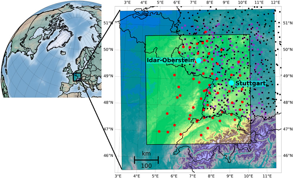
FIGURE 1. Overview of the WRF domain with evaluation area (bright area), synoptic stations (black dots), additional precipitation stations (purple crosses), GNSS stations (red dots) and radiosonde stations (blue dots).
A total of approximately 250 synoptic stations and further 100 precipitation stations from the German Met. Service (DWD) located within our domain serve as basis for validation and partly assimilation means. These stations are quality controlled and only available for the German part of the domain (black dots and purple crosses in Figure 1). The variables relative humidity, temperature, pressure and precipitation are considered.
Data from radiosondes are provided by the Integrated Global Radiosonde Archive (IGRA) homepage (IGRA, 2022). There are two radiosonde stations in the area where observations were assimilated. The Idar-Oberstein radiosonde offers measurements every 6 h in the western part of the domain and the Stuttgart radiosonde, located a bit more to the south-east, provides ascent data every 12 h for all episodes (blue dots in Figure 1). A comprehensive set of quality controls was applied to remove gross errors from radiosonde data (Durre et al., 2006). A variety of meteorological variables such as pressure, temperature and humidity were obtained at different altitudes varying with each sounding.
GNSS Data
Data of the GNSS Upper Rhine Graben Network (GURN) are used in this work. The GURN consists of 66 stations and their GNSS observations were processed with the GAMIT/GLOBK software (V10.7) (Herring et al., 2018). Several advanced models were used: For instance, the state-of-the-art Vienna Mapping Function 1 (Boehm et al., 2006) and the a priori zenith hydrostatic delay from the European Centre for Medium-Range Weather Forecasts (ECMWF) (Simmons and Gibson, 2000). The tropospheric delay was estimated as Zenith Total Delay (ZTD) every hour together with north and east gradients every 12 h. The higher-order ionospheric delay was modeled with ionospheric data from the Centre for Orbit Determination in Europe (Schaer and helvétique des sciences naturelles. Commission géodésique, 1999) and the International Geomagnetic Reference Field 12 (Thébault et al., 2015). The cut-off angle was set as 10° and the observations were weighted according to their post-fit phase residuals. The IGS final orbits and ITRF2014 reference frame (Altamimi et al., 2016) were used. Solid Earth tides, ocean tides, and pole tides were conventionally modeled and corrected. The GNSS-derived ZTD estimates can be split into two parts: Zenith Hydrostatic Delay (ZHD) and Zenith Wet Delay (ZWD). The ZHD are estimated with the Saastamoinen model (Saastamoinen, 1972). The GNSS-derived ZWD is calculated as the differences between the ZTD and ZHD. Then, Precipitable Water Vapor (PWV) is retrieved from the GNSS-derived ZWD:
where ρw is the density of liquid water (in kg m−3); Rw is the gas constant for water vapor (in J kg−1 K−1),
in which ei and Ti denote the average vapor pressure (in hPa) and average temperature (in K) of the atmosphere at the ith layer, respectively, and Δhi denote the atmosphere thickness of the ith layer (m). The ith layer of the atmosphere indicates the atmosphere between the ith and (i + 1) th pressure level. The vertical profiles of relative humidity and temperature obtained from ERA5 datasets were used to calculate Tm. For more details on the calculation, readers are referred to (Yuan et al., 2021).
WRF Model
The WRF Model (version 3.9.1.1) (Skamarock et al., 2008) was applied in this investigation as a limited area model (LAM) to downscale global atmospheric reanalysis data. The setup of physical parametrization schemes was widely adopted from another work in this region (Wagner et al., 2018). The respective list of selected parameterizations is summarized in Table 1. The ERA5 reanalysis dataset (Hersbach et al., 2020) with an hourly resolution provided the forcing data at our WRF domain boundaries. Due to its high spatial resolution of approximately 31 km and 138 vertical model levels we directly downscaled to our target domain. In this way we omitted intermediate domains which may falsify main circulation patterns and reduced computational time.
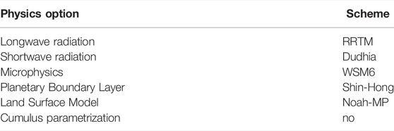
TABLE 1. WRF Model settings: RRTM (Mlawer et al., 1997), Dudhia (1989), WSM6 (Hong and Lim, 2006), Shin and Hong (2013), and Noah-MP (Niu et al., 2011).
For the model domain in Figure 1 we used a mesh of 309 × 319 grid cells with 2.1 km horizontal resolution and 72 vertical eta levels which were spaced according to the WRF standard method. We only evaluated the inner area of 209 × 219 cells to exclude possible boundary artifacts from the analysis (bright area in Figure 1) due to the large grid scaling factor.
Assimilation
WRF features 3D and 4D variational data assimilation schemes. 4D VAR is computational more expensive, but enables assimilations at the exact time of observation whereas 3D VAR uses a single assimilation time (Barker et al., 2003; Barker et al., 2004). In addition to the variational assimilation schemes, respective hybrid schemes exist in WRF with an additional Ensemble Transform Kalman Filter (ETKF) component. The benefit of the hybrid system is that the static (background) covariances of the variational schemes are combined with ensemble covariances to estimate the complex, flow-dependent forecast-error statistics (Wang et al., 2008a; Wang et al., 2008b). Since we consider only episodes with a duration of several days and observations exhibiting the same temporal resolution as our assimilation frequency, we selected the 3D VAR scheme for our study.
Data assimilation merges numerical weather prediction (NWP) states and observations considering their respective error statistics to achieve an improved initial state. Variational data assimilation schemes accomplish this step by iteratively minimizing the following cost function (Ide et al., 1999; Barker et al., 2003; Barker et al., 2004):
Based on the background field xb and the observations (y), an improved estimate of the atmospheric state x is obtained based on maximum likelihood principles. H denotes the forward observation operator, used to transform the model variables into observations’ space. All observations, in 3D VAR, refer to the same time. R represents the observation error covariance matrix containing information about observations’ errors and their correlation. B denotes the corresponding covariance matrix for the background error.
The background error covariance matrix is calculated separately for each of the selected episodes based on the NMC-method (Parrish and Derber, 1992). Therefore, averaged forecast differences of the 12 and 24 h forecast (valid at the same time) of month-long WRF simulations were applied. The simulations were performed for the same month in which each of the episodes occurred and with the same setup as our open cycle simulations. In this way we derived necessary statistics which best fitted our target region and episode. For the background error option cv5 the control variables streamfunction, unbalanced velocity potential, unbalanced temperature, pseudo relative humidity, and unbalanced surface pressure are used. The pseudo relative humidity is defined as the quotient of specific humidity and saturated specific humidity from the background field. The difference to the cv6 option is this moisture control variable. In cv6 this variable is the unbalanced portion of the pseudo relative humidity (Wang et al., 2015).
There are many factors influencing the quality of GNSS assimilations in LAMs. The calculation of ZTD from slant delays involves uncertainties as well as the applied observation operator in the model (Singh et al., 2019). Differences between exact station altitude and model altitude is a further source of uncertainty. The calculation of ZHD within the model has to be taken into account, since model top from LAMs are usually significantly lower than, for example, reanalysis data (Lindskog et al., 2017). Therefore, bias correction is usually performed. The common approach is to apply a mean correction (Bennitt and Jupp, 2012; Rohm et al., 2019; Giannaros et al., 2020) to correct a possible offset. Arriola et al. (2016) presented a variational bias correction which treat possible errors much more flexible, but it is currently not implemented in WRF.
In our study, we had a thorough look at this data base, before we assimilated ZTD data. Firstly, we compared GNSS data with our forcing data ERA5 for the spring episode and also for the entire year of 2016 based on ZTD. Small biases between ±4 mm and only two stations with a maximum bias of −7 to −8 mm were obtained for all stations which were used in our assimilation experiment. According to Eq. 4, the calculation of ZHD in WRF is not dependent on the model top, so that additional corrections are not considered necessary:
with pWRF pressure from WRF model, height h and latitude φ of a GNSS station. More information about the observation operator can be found in Rohm et al. (2019).
Secondly, tests assimilating ZTD and PWV provide similar results. Consequently, the treatment of ZHD by the observation operator works well and no additional uncertainties are obviously induced by assimilation. For both simulations over 95% of observations pass the quality control mechanisms in the WRF assimilation system. Only inconsistencies in GNSS station heights turned out to be very sensitive for assimilation results. Taking into account the exact station elevations (including tower or building, if necessary) removed inconsistencies. Furthermore, we used the TEQC software (Estey and Meertens, 1999) to check the quality of raw GNSS observations and excluded low-quality observations. We did not perform any further bias correction for our experiments, because of two reasons: 1) only minor ZTD biases were obtained, when compared to ERA5; 2) uncertainties may be introduced into the system when mean biases are calculated from simulations without assimilation (i.e., open cycle runs) or from other datasets. Our results show that there is a feedback of ZTD assimilation on temperature which in turn impacts the calculation of humidity (profiles) in WRF. In a combined assimilation with temperature this may lead to inconsistencies if ZTD was bias corrected in advance.
Selection of Episodes and Experiments
Four episodes were selected for evaluation according to the following criteria: 1) representing typical weather conditions of the region and season, 2) including wet and dry days, 3) a moderate amount of rain in the whole domain and 4) good data availability. An overview of rain characteristics and driving meteorological mechanism for each episode is shown in Table 2. The spring episode lasted from 11 to 22 of April 2016 and showed a mean precipitation amount of 35 mm especially until the 16 of April with partly convective activity. This spring episode was chosen to test the different options for assimilation. The summer episode (13–23 of July 2018) is characterized by highly variable convective conditions in space and time, although only a mean of 15 mm of total rainfall was observed based on the precipitation stations in our domain. The autumn episode lasted from 16 to 31 of October 2018. The observed 20 mm of precipitation was mainly obtained at the end of the episode with moderate intensities, from October 27 on. The winter episode (6–20 of January 2017) showed light precipitation from 9 to 17 of January with mean amounts of 30 mm. The latter three episodes were used to test whether the obtained best assimilation setup for spring adds value for simulations of other seasonal periods.
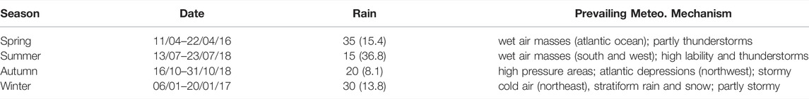
TABLE 2. Overview of chosen episodes with date, rain mean [mm] (maximum intensity [mm/h]) and driving meteorological mechanisms. Rain values are derived from German precipitation stations.
An hourly update cycle was used for the ERA5 data for all simulation experiments. To allow for the slow temporal spinup of soil related model variables, a preliminary so-called “open cycle” simulation over several weeks was done before each episode. These simulations were performed without assimilation, but with the same settings as the assimilation runs. They provided the initial conditions at the lower boundary for the subsequent assimilation runs. In order to test the impact of the assimilation of observations, the open cycle simulations serve as basis for comparison for our assimilation experiments. Unless explicitly mentioned otherwise, only the first forecast hour is evaluated in this study. In this way assimilation usually show largest impact and meteorological variables in the model should be in balance. This particularly applies to the comparison of moisture and precipitation values at the same time. The assimilation of observations modifies only the moisture variables, but not precipitation. In Table 3 an overview of the different experiments is given, with applied abbreviation, episode dates, assimilation variables and special settings.
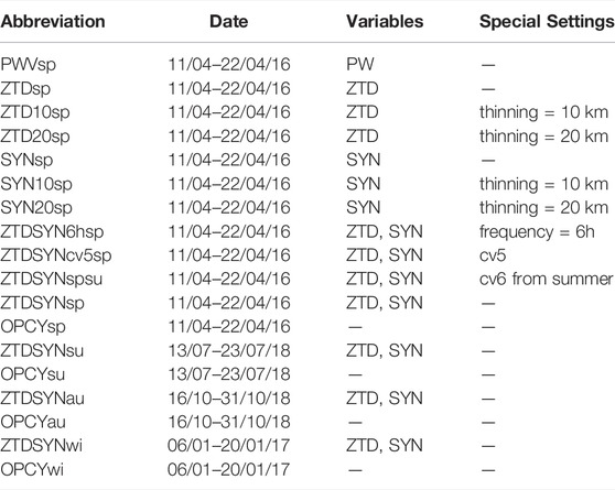
TABLE 3. Overview of assimilation experiments with abbreviations representing the assimilated observations: e.g., OPCY = open cycle, ZTDSYN = synoptic and ZTD data with the following additions: 10 (thinning distance of 10 km), 6 h (6 h cycling rate), cv5 (cv5 BE option), sp, su, au, and wi (spring, summer, autumn, and winter); additionally, date, assimilation variables and special settings are revealed.
Statistical Measures
Besides common statistical measures such as mean error or standard deviation, the Kling Gupta-efficiency (Gupta et al., 2009) is applied:
where
This goodness-of-fit measure combines three well-known metrics which can be used to describe the accordance of two variables: The correlation (cor) showing the relative relationship, the quotient of the respective standard deviations (dsd) revealing the variability bias (qd) and the quotient of mean (mean) comparing the magnitudes of two datasets (qm; mean bias). The KGE values range between –Infinity and +1. According to Knoben et al. (2019), an improvement compared to the average value is obtained if KGE > −0.41.
Precipitation shows a very high temporal and spatial variability, and the comparison of model pixels with point data from stations brings additional uncertainties. Categorical skill scores such as probability of detection (POD), false alarm ratio (FAR) and frequency bias (FBI) were therefore used for the comparison with precipitation stations (Wilks, 2011). In addition, a subdivision was made according to light (0.1–2.5 mm), moderate (2.5–10 mm) and heavy precipitation (
with uppercase and lowercase denoting observed event and prediction, respectively.
The probability of detection in Eq. 7 gives the number of correct hits compared to total observations. A value of 1 is optimal. The false alarm ratio in Eq. 8 gives the number of false positives in total predictions. Small values are desirable. The frequency bias in Eq. 9 compares the “total forecast yes” with the “total observed YES.” Values greater than 1 are overforecast, less than 1 are underforecast.
A bootstrap technique was used to determine the significance of the evaluations. According to Wilks (2011) and Bliefernicht et al. (2019), the time series of observations and simulations are recalculated from old pairs of values by random selection with replacement. This was repeated 1,000 times. Then, the contingency tables were derived from each new pair of time series and the categorical skill scores were recalculated. The confidence interval with a level of 95% then resulted from the 5 and 95% percentile of these distributions. If the contingency intervals of two experiments overlap, the differences are considered non-significant.
Results
Assimilation Variable
In WRF the assimilation of both, PWV and ZTD are possible. Hence, we start with a comparison of assimilation results for these two variables.
Figure 2 gives an overview of the performance of all simulation experiments compared to precipitation time series of 350 stations in the German part of our domain separated into light (0.5–2.5 mm; A) and moderate rain (2.5–10 mm; B). The colored bars indicate the confidence intervals of the respective experiment regarding the three different skill scores POD, FAR and FBI. This evaluation is only performed for light and moderate rain, since there are too few pairs of value for heavy rain. The assimilation of ZTD resulted in a better FAR and FBI (ZTDsp in Figure 2A). Small improvements are also obtained for POD (light rain) and moderate rain skill scores but without significance (Figure 2B).
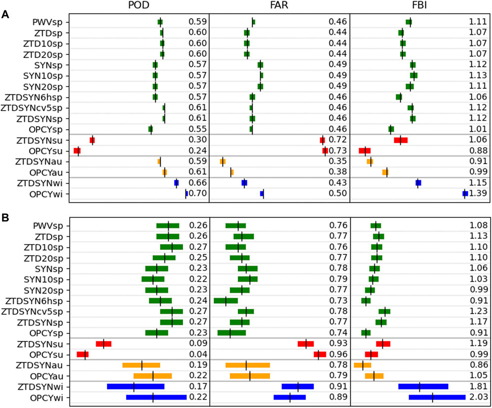
FIGURE 2. Comparison of all simulations with hourly precipitation amounts at approx. 350 stations regarding POD, FAR and FBI for (A) light rain (0.1–2.5 mm/h) and (B) moderate rain (2.5–10 mm/h). Confidence intervals (95%) of the respective simulation are presented as color bars. With abbreviations representing the assimilated observations: e.g., OPCY, open cycle; ZTDSYN, synoptic and ZTD data with the following additions: 10 (thinning distance of 10 km), 6h (6 h cycling rate), cv5 (cv5 BE option), sp, su, au, and wi (spring, summer, autumn, and winter).
Deviating results were obtained for the comparison with radiosonde data for the location Stuttgart. According to Figure 3B, on average, the assimilation run with PWV is slightly better than the corresponding ZTD run. A closer inspection shows that there are periods of time in which one or the other variant performs better. According to Figure 3A, the main differences with respect to the mixing ratio (MR), occur at altitudes below 4,000 m. This is also where the main water vapor resides and, in the first half of the episode, where rain is falling. Higher values for the mixing ratio in the profile for ZTD (Figure 3A) are usually linked with peaks in the integral values of PWV (not shown). The variations of the mixing ratio go along with those of temperature (T). Figure 3C reveals a clear impact on temperature, also for the first part of the episode. Variations with height and slightly higher temperatures were observed by assimilating ZTD. The impact was visible also for higher altitudes.
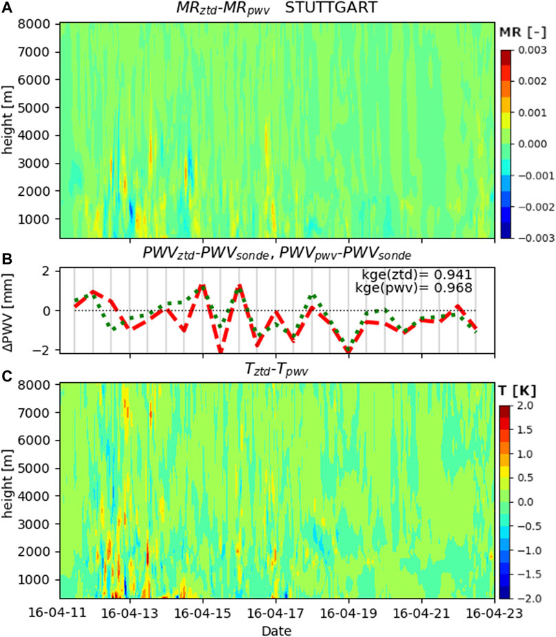
FIGURE 3. Difference of the mixing ratio (MR) with height (A) and temperature (T) (C) for assimilating ZTD (red) and PWV (green) at the Stuttgart location for the spring episode and difference of corresponding PWV values and radiosonde data (B).
Data Thinning
Data thinning is a necessary procedure, when the background error correlations are not additionally considered and when the spatial density of data to assimilate is very high, at least below 10 km. The spatial distance of the GNSS stations used here is typically larger than 20 km, with a few pairs of stations spaced less than 10 km apart. Synoptic stations exhibit a much higher spatial density, often below 10 km.
We performed six simulations which are briefly evaluated in the following: three for assimilating ZTD with thinning distances of 10 and 20 km, and without data thinning. Additionally, the same procedure was applied to three assimilation runs of synoptic data (SYN).
The comparison of SYN with radiosonde data reveals smaller mean errors for a thinning distance of 10 km but slightly increased standard deviations (Figures 4A,B). For ZTD the improvement is less clear with a slight decrease of the standard deviation for 10 km thinning distance (Figures 4C,D). These small differences appear at altitudes of approx. 2,000 m. The comparison with precipitation stations don’t show reliable differences among the various simulations of SYN or ZTD. For light rain (Figure 2A; bars 2–7) no differences are found and for moderate rain (Figure 2B; bars 2–7) only tendencies are observed, which are not significant.
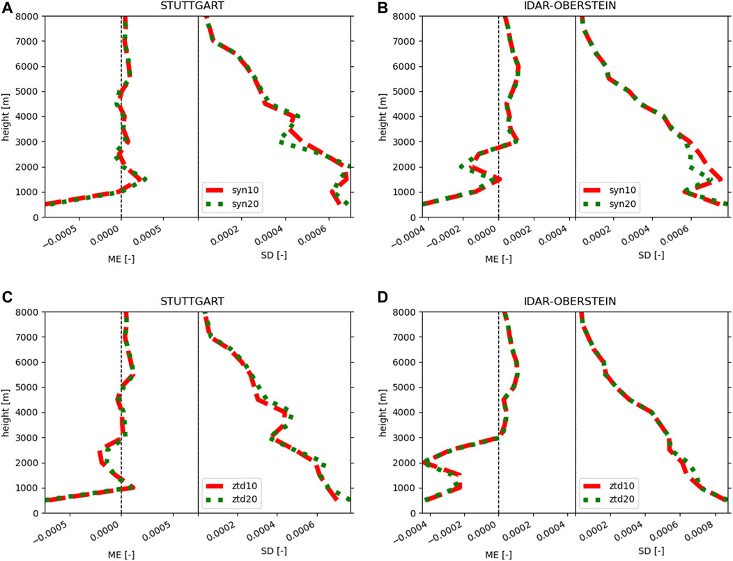
FIGURE 4. Mean error and standard deviation of the mixing ratio profile for the spring episode comparing the assimilation of synoptic data with thinning distances of 10 km (red) and 20 km (green) with radiosonde data from Stuttgart (A), Idar-Oberstein (B) and the respective results for assimilating ZTD for both locations (C,D).
Assimilation Frequency
In principle, the temporal assimilation cycle rate determines how closely the simulation is coupled to the observations. If the assimilation of observations adds value, then a higher rate of assimilation should lead to better simulation performance. To evaluate this aspect, we performed simulations with assimilation of ZTD and synoptic station data using an assimilation frequency of 1 and 6 h, respectively. Indeed, a higher rate of assimilation improves the POD with precipitation stations as shown in Figure 2A (ZTDSYN6hsp vs. ZTDSYNsp) with a slightly higher FBI value. The differences for moderate rain (Figure 2B) are not significant, but show the same tendencies. The mean KGE at the radiosonde location for the column integrated value of PWV is higher for the hourly assimilation rate at Idar-Oberstein (Figure 5F), but lower at Stuttgart (Figure 5B). Systematic differences were obtained for the mixing ratio profiles shown in Figures 5A,E; below 1,500 m the mixing ratio based on the hourly assimilation rate is lower, but at about 2000 m an obvious increase of mixing ratio values becomes apparent. This characteristic is constant throughout the whole episode and therefore widely independent of the meteorological situation. The results for temperature (Figures 5C,G) reveal similar patterns with low variations above 2000 m, an area of transition between 1,500 and 2000 m and obvious differences below. In these lower 2000 m, the daily cycle becomes apparent, but not at higher altitudes. One obtains weaker, but similar patterns for the comparison of the 6 hourly cycle run with the open cycle simulations (Figures 5D,H). Consequently, this feature is not an effect of the assimilation rate. It is rather the result of the strong influence that assimilation has essentially in the lower 2,000 m of the atmosphere, with little impact on the layers above.
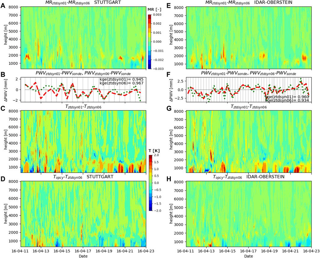
FIGURE 5. Difference of the mixing ratio (MR) with height (A) and temperature (T) (C) for the combined assimilation of ZTD and synoptic data at the Stuttgart location with 1 h (red) and 6 h (green) resolution for the spring episode and difference of corresponding PWV values and radiosonde data (B). (D) shows the respective comparison of the open cycle run and the combined assimilation of ZTD and synoptic data with 6 h cycling rate for temperature. (E–H) are the respective comparisons for Idar-Oberstein.
An added value of a higher assimilation rate becomes obvious when considering the comparison with radiosonde profiles also for altitudes below 2,000 m (Figure 6) with lower mean errors and standard deviations.
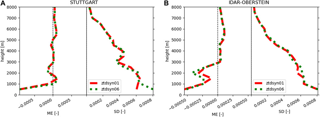
FIGURE 6. As in Figure 4, but for the comparison of the assimilation of ZTD and synoptic data with 1 h (red) and 6 h (green) cycling rate at the Stuttgart (A) and Idar-Oberstein (B) location.
Best Setup
In order to identify the optimal setup and also to find the main reason for the sudden change of assimilation patterns at elevation about 2,000 m above ground presented in Figure 5, the assimilation of synoptic and ZTD data was evaluated independently. One does not see an additional positive effect when assimilating SYN only or ZTD only for the comparison with precipitation stations (Figure 2, SYNsp/ZTDsp vs. OPCYsp) and the mean PWV at Stuttgart (Figure 7). The contour plot of Figures 7A,C clearly reveals that the assimilation of synoptic data is mainly responsible for the distribution of patterns above and below 1,500–2000 m also apparent in Figure 5. Synoptic stations influenced assimilation results mainly up to a height of 2,000 m with a maximum between 1,500 and 2,000 m in this evaluation. The assimilation of ZTD leads to much smoother differences of the mixing ratio with height, although the main effects are also observed below 2,000 m (Figure 7C).
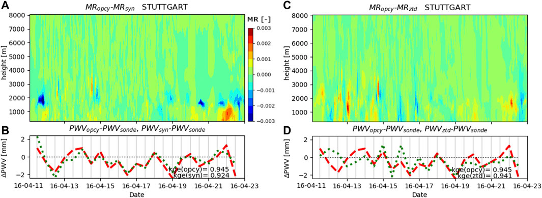
FIGURE 7. Difference of the mixing ratio (MR) with height at the Stuttgart location for the spring episode, comparing the open cycle simulation (red) with assimilating (A) synoptic data only (green) and (C) ZTD only (green) and difference of corresponding PWV values and radiosonde data (B,D).
The individual assimilation of both datasets shows drawbacks for certain time steps as can be seen from Figures 7B,D. Those variations often compensate each other. Overestimation due to the assimilation of one variable coincide with underestimations due to the other variable. The contour plots of Figure 7 support these findings and furthermore show that these variations occur usually at similar altitudes; overestimations in Figure 7B when assimilating SYN are mostly compensated by lower values based on the ZTD assimilation (Figure 7C) and vice versa. The evaluation of the ZTDSYN-experiments are jointly addressed for all episodes in subsection Seasonal Differences.
Background Error
The background error (BE) strongly influences how observations are assimilated into the model. The prerequisite for a successful assimilation is the correct temporal interaction of BE and assimilation period. In Figure 8 we show the impact of a BE obtained in spring and one in summer for the spring episode. For the integral PWV values (Figure 8B) moderate variations were obtained with a higher KGE (0.945 vs. 0.905) for the correct interaction of spring BE and spring episode. Additionally, significant shifts of water vapor in the vertical profile became apparent which can strongly influence the generation of precipitation.
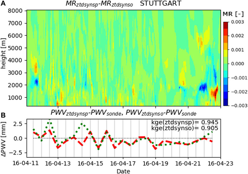
FIGURE 8. Difference of the mixing ratio (MR) with height (A) for the combined assimilation of ZTD and synoptic data based on the BE obtained in April 2016 (spring episode, red) and the BE obtained in July 2018 (summer episode, green) at the Stuttgart location for the spring episode and difference of corresponding PWV values and radiosonde data (B).
In addition to the temporal correspondence of the BE, the BE option determines how assimilated variables are treated within the model. In WRF the multivariate cv6 option considers also feedback mechanisms of assimilated variables on other meteorological quantities which are physically dependent. This allows feedback of temperature on water vapor and thus probably enables a faster temporal spinup in the model with updated initial conditions. In theory, the cv6 option should be superior compared to the cv5 option, especially for high assimilation frequencies and when water vapor is assimilated.
No significant differences for the comparison with precipitation stations are observed. Tendencies of improvement for the cv6 option and moderate rain are shown for FAR and FBI (Figure 2B). Figure 9 indicates that there are only minor differences between both simulations at the radiosonde’s locations, thus a closer look at individual timesteps is necessary. At 14th of April at 4 p.m. a shift of mixing ratio with height becomes apparent in Figure 9A. The cv6 option shows an increase of water vapor at about 1,400 m, but a reduction at 3,800 m. This does not necessarily change the integral PWV value but can influence the generation of precipitation, when moisture saturation is reached at certain levels or not. The differences in PWV at the radiosonde locations are indeed almost negligible.
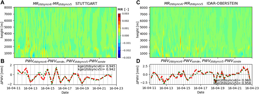
FIGURE 9. Difference of the mixing ratio (MR) with height (A) for the combined assimilation of ZTD and synoptic data based on the cv6 BE option (red) and the cv5 BE option (green) and bias of corresponding PWV values and radiosonde data for Stuttgart (B) and Idar-Oberstein (C,D).
Figure 10 shows a comparison of vertical profiles at the Stuttgart site for time step 14th of April 2016 12 p.m., when only temperature is assimilated. For altitudes below 5,500 m the mean error is widely reduced with the cv6 option. This clearly reveals the benefit that temperature can have on water vapor through feedback when applying the cv6 option.
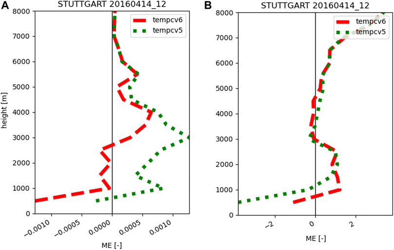
FIGURE 10. Mean error of the mixing ratio (A) and temperature (B) for the 14th of April 2016 12 p.m. comparing the assimilation of temperature only with radiosonde data, based on the cv6 BE option (red) and the cv5 BE option (green) for Stuttgart.
Seasonal Differences
Based on the best identified setup for assimilating synoptic stations and ZTD from GNSS stations with the cv6-option (ZTDSYN), we run simulations for four episodes in four different seasons. We investigate whether improvements can be achieved by assimilation for each season.
In Figure 11, the profiles of simulated mixing ratios are compared to radiosonde data at Stuttgart for every available time step and evaluated for their mean error and standard deviation. The respective profiles for Idar-Oberstein are shown in Figure 12. During the spring episode, assimilation mainly affects the mixing ratios at altitudes below 3,000 m, improving the mean error and standard deviation. In winter, the improvement was somewhat smaller, but still noticeable below 3,000 m. Overall, the greatest improvements were achieved in the summer months and also at higher altitudes. Almost no effect of assimilation is apparent in autumn.
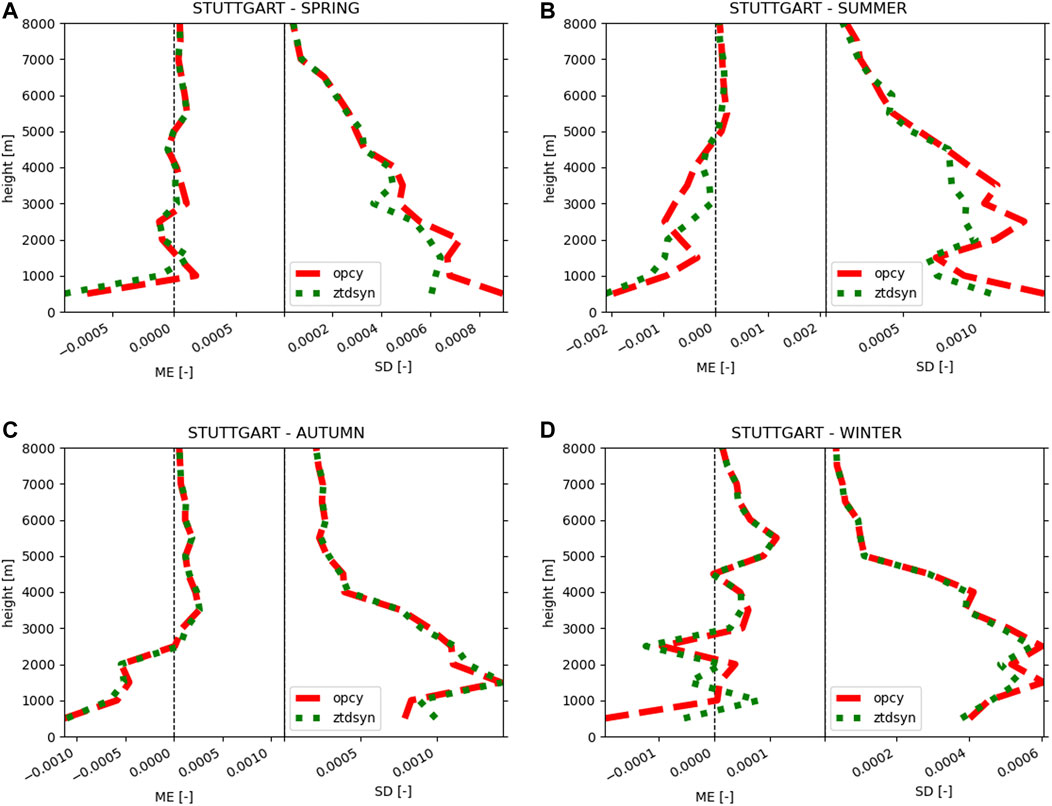
FIGURE 11. As in 4, but for the open cycle simulation (red) and the assimilation of ZTD and synoptic data (green) in spring (A), summer (B), autumn (C) and winter (D).
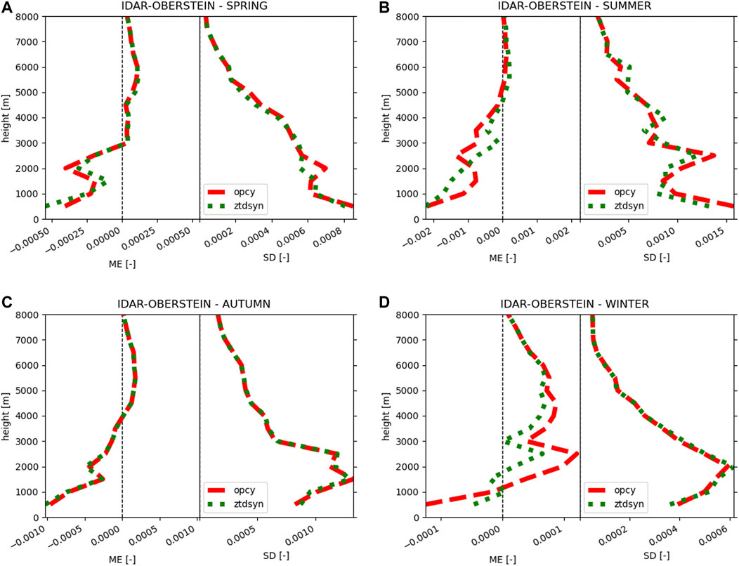
FIGURE 12. As in 4, but for the open cycle simulation (red) and the assimilation of ZTD and synoptic data (green) in spring (A), summer (B), autumn (C) and winter (D) at Idar-Oberstein.
The assimilation increased precipitation amounts in spring and summer. One indication for this is that the number of forecasts of light and moderate rain are increased in Figure 2 (FBI, ZTDSYN vs. OPCY, green and red bars). In autumn and winter precipitation amounts are reduced by assimilation and also FBI is getting smaller (yellow and blue bars). The POD is improved by assimilation in spring with no effect on FAR and in summer both POD and FAR are improved. In autumn FAR is improved, but not POD. In winter the high FBI is reduced by assimilation which leads to improvements of FAR, but again a lower POD value. These results are mainly based on light rain (Figure 2A) since moderate rain evaluations reveal similar results, but are usually not significant.
Water Budget
In order to evaluate the impact of assimilation on the water budget and to understand the mechanisms which may modify the respective components, the mean sub-daily evolution of evapotranspiration, net radiation, latent heat and sensible heat of the domain mean was analyzed first. In Figure 13 we compare results for the spring episode originating from the open cycle simulation, the assimilation of GNSS data and synoptic station data, and GNSS data only. If only GNSS data was assimilated (ZTD), evapotranspiration (ET) remains almost unchanged. Though, due to the increase of atmospheric water vapor in the spring episode, cloudiness is probably enhanced and solar radiation is reduced at the surface, leading to smaller surface fluxes. This effect can be seen by a reduction of net radiation in the model and an increase of precipitation (PREC) in spring (Table 4). The reduced net radiation fluxes at the surface are shown by slightly reduced latent heat and sensible heat fluxes around noon. The additional assimilation of synoptic station data (especially temperature) shows a direct impact on evapotranspiration and also feeds back to net radiation (Figure 13A). Energy fluxes are modified, showing a reduction of sensible heat (SH) and an increase of latent heat (LH) during daytime compared to the open cycle simulation (see Figure 13B). In this way, a small additional impact of evaporation on precipitation is possible.
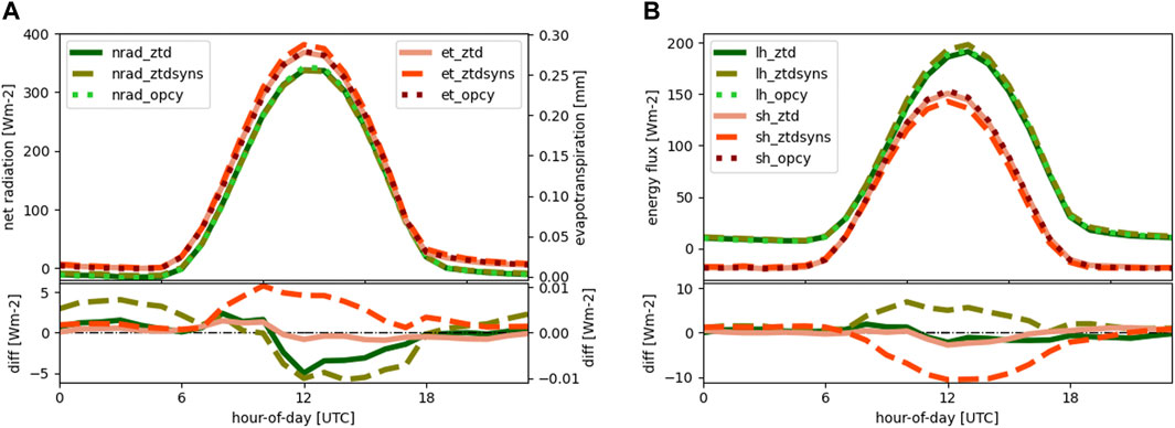
FIGURE 13. Daily cycle of the domain mean regarding net radiation (nrad) and evapotranspiration (et) (A), and sensible heat (sh) and latent heat fluxes (lh) (B) for the open cycle simulation (opcy), best assimilation setup (ztdsyn) and assimilating ZTD only (ztd) for the spring episode.
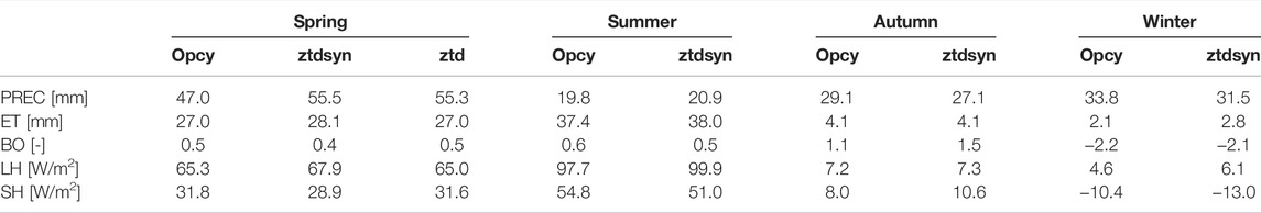
TABLE 4. Water cycle and energy budget components from simulations without assimilation (opcy), best assimilation setup (ztdsyn) and assimilating ZTD only (ztd, only spring) for our four episodes in every season considering the domain mean.
The same mechanisms and effects of assimilating GNSS and synoptic station data become apparent for the other seasons (Table 4). The summer episode is comparable with the spring episode, showing a reduction of the Bowen-ratio (BO, ratio of sensible heat and latent heat) and an increase of precipitation and evapotranspiration. In autumn, precipitation is reduced and no effect on evapotranspiration is observed. Yet, the Bowen ratio is increased since only sensible heat is increased, not latent heat. In winter, precipitation is also reduced by assimilation. Latent heat and therefore evapotranspiration is increased, but since sensible heat is also increased the Bowen ratio shows only minor changes.
Discussion
We chose a thinning distance of 10 km, which is in accordance with the results presented in Mile et al. (2019). The differences in our evaluations are small and not significant, but in our study region only very few GNSS stations are affected by spatial thinning and still we see certain differences. For other domains the optimal thinning distance might vary due to differences of model grid spacings, temporal resolution and assimilation variables or their respective quality. Our results show that it is worth to take this aspect into consideration.
More frequent observations of good quality should improve the forecasts. This is not always the case. Differences between simulation and observations or even biases of observations can propagate deeper into simulation results due to a higher assimilation frequency and thus increase the discrepancy between model and reality. For example Nykiel et al. (2016) also showed comparisons for 1 and 6 h assimilation cycling rates. According to their results, the 6 h cycle performs better than the 1 h cycle. They claimed that the model needs a certain spinup time to reach stable conditions after changing the initial state which seems to be not satisfyingly fulfilled by the 1 h frequency simulation. If such effects occur, the use of Digital Filter Initializations [DFI; (Skamarock et al., 2008)] may reduce potential initial model imbalances, but this was not tested within this study. Based on the analysis of the simulations presented here, such effects were not evident. Improvements due to a higher assimilation rate prevailed. The reason is that for certain individual time steps the assimilation clearly brings added value. If assimilation times do not match with these time steps, important observations might get ignored and thus potential improvements reduced. It is possible, that a compromise between the applied assimilation frequencies of 1 and 6 h performs best. We did some tests with a 3 h assimilation frequency, but differences between 1 and 3 h frequencies were not significant.
If reducing spinup times potentially deteriorates the simulation results, the choice of the background error option can mitigate detrimental effects. In WRF, the multivariate cv6 option considers also feedback mechanisms of assimilated variables on other meteorological variables which are physically dependent. This allows, for instance, feedback of temperature on water vapor and probably leads to a faster temporal model spinup due to updated initial conditions. This is the main reason why the multivariate BE option cv6 showed benefits compared to the cv5 option. Hints for that behaviour can be found in the faster and often more intense reaction of PWV for cv6 in Figures 9B,D when observed PWV values change. Another advantage of the BE option cv6 compared to the cv5 option is that for individual time steps the assimilation of only temperature can have a significant benefit on water vapor results.
However, the BE comprises more than just different BE options. Especially the temporal dependence of the BE is important. Poli et al. (2007) reported convergence problems for some minimizations when observation error estimates are applied in summer which were calculated for another season of the year. They showed that the ZWD assumed background error reveals a strong seasonal dependence and concluded that adjustments are necessary for summer episodes. Our results confirm these findings. It is therefore important to use a BE that is suitable in terms of time, location (domain-dependent) and also for the assimilated variables (BE option) for performing the simulation. The hybrid background error techniques found in WRF are a very promising set of tools for future studies in this respect: A flow-dependent estimation of the background error statistics is implemented there by combining static and ensemble-estimated error covariances (Wang et al., 2008a; Wang et al., 2008b).
Regarding the choice of variables, the assimilation of ZTD offers advantages as compared to PWV. Slightly improved results were obtained and no additional pre-processing is required. The differences as compared to the assimilation of PWV are minor and not every model system provides an operator for assimilating ZTD. ERA5 is used for both, the calculation of PWV from GNSS data and also as forcing data for WRF. Correlated errors in the PWV assimilation experiment may explain the better performance of ZTD, though ERA5 provides forcing data only at the domain boundaries. No differences were found between mean temperature profiles at the radiosonde locations (not shown). Either ZTD or PWV must be used in WRF, when simultaneously GNSS stations and for instance InSAR data are assimilated. There is no evidence in our results against the use of PWV. Assuming equivalent ZHD calculations for both the preparation of PWV from GNSS measurements and the separation of ZTD into ZWD and ZHD in WRF, the differences between PWV and ZTD are only related to pressure and temperature. Pressure is usually very conservative, so that differences arise mainly due to temperature. The positive influence of the additional assimilation of temperature can be interpreted exactly in this direction: a meaningful assimilation of water vapor on the basis of ZTD is only guaranteed by reasonable temperature data. Therefore, it is advisable to assimilate temperature data at the same time when assimilating ZTD.
The effect of assimilating ZTD and synoptic station data simultaneously can be seen in our best assimilation setup. The assimilation of synoptic stations lead to larger variations with altitude at heights between 1,500–2,000 m, which can also lead to deterioration compared to open cycle simulations. The additional assimilation of ZTD often reduced these falsified patterns. However, there is no guarantee that such a simultaneous assimilation of different variables always yields added value; this should be evaluated for each individual setup. Here, the reliability of temperature data plays an important role.
In general, improvements are possible for all seasons based on such an optimal setup, even though the impact on mean statistical values might be small. The reliability of the obtained differences (confidence intervals) is often large due to the short duration of our episodes. Additionally, radiosonde data is only available every 6 or 12 h. We applied an update cycle of 1 h for ERA5 which restricted the self-development of meteorological patterns in WRF. Choosing an update cycle of 6 h instead of 1 h may therefore also lead to a larger impact of assimilation. The added value by assimilation is usually much higher for individual time steps. It also needs to be noted that no significant deterioration was observed by assimilation. The seasonal results show that it is very important to have an open cycle simulation as reference to evaluate potential benefits of the assimilation process. In autumn, very good results and high agreement with validation data were already obtained with the open cycle simulation leaving almost no room for further improvement. The same holds true for winter, where the improvement by assimilation was limited to the reduction of humidity in the model and an improved false alarm ratio. In summer, convection with high temporal and spatially variability is very difficult to model in space and time, so assimilation of observations is most promising for such episodes and the largest improvements can be obtained there. Since improvements are often difficult to achieve for other rain episodes, a thorough selection of assimilation options may determine whether a simulation is improved by assimilation or not.
We only evaluated a selection of possible influencing factors and corrections in this study. The use of more variable bias corrections of GNSS data is very promising. Arriola et al. (2016) successfully applied a variational bias correction and showed the advantages compared to a static one. Additionally, many forward observation operators show potential of improvement. Singh et al. (2019), Singh et al. (2021) introduced an improved observation operator which takes also hydrometeors into account.
Our evaluation of the water budget shows the main impact of the assimilation of GNSS data and temperature on simulation results and the two associated effects: The assimilation of water vapor data (e.g., GNSS, InSAR, etc.) can lead to a modification of precipitation amounts when saturation excess is reached. This usually also has an impact on runoff, which has not been evaluated in this study. In contrast, the assimilation of temperature data or any other source of energy (e.g., radiation) is able to modify the energy fluxes and impacts the water balance primarily through evaporation. However, a small impact on precipitation is also possible through feedback, which leads to an additional improvement in our experiments. Consequently, all components of the water cycle can be strengthened or weakened by the assimilation process depending on the differences between model state and assimilated observational data.
Conclusion
This study showed that the best assimilation setup is a combination of parameter selection, spatial thinning, assimilation frequency and background error settings. The high spatial and temporal resolution of 10 km and 1 h shows that the added value of high information density largely outweighs possible observational error correlations. Improvements in overall performance are achieved, in particular, through the joint assimilation of water vapor and energy variables such as temperature. By choosing the corresponding multivariate background error option cv6, we were able to achieve an improvement for each of the episodes considered here. The evaluation of the water cycle shows that all components of the water cycle can be affected by our assimilation tests.
In general, the consideration of feedback processes between water vapor and energy variables during assimilation seems to have further potential for improvement and it is certainly worthwhile to investigate this aspect further in the future.
Data Availability Statement
The raw data supporting the conclusion of this article will be made available by the authors, without undue reservation as far as data is available (simulations) and upon reasonable request.
Author Contributions
BF, HK and TR contributed to the conception and design of the study. PY created the GNSS dataset and wrote the GNSS data section. AW prepared the input datasets, carried out the simulations and performed the analysis. All authors revised and approved the submitted version.
Funding
The research was conducted in the framework of the AtmoWater project (No. KU 2090/10-1, project number: 321886779), with the financial support of the DFG (German Research Foundation). This work was additionally supported by the LANDKLIF project. The LANDKLIF project is sponsored by the Bavarian State Ministry of Science and the Arts in the context of the Bavarian Climate Research Network (bayklif).
Conflict of Interest
The authors declare that the research was conducted in the absence of any commercial or financial relationships that could be construed as a potential conflict of interest.
Publisher’s Note
All claims expressed in this article are solely those of the authors and do not necessarily represent those of their affiliated organizations, or those of the publisher, the editors and the reviewers. Any product that may be evaluated in this article, or claim that may be made by its manufacturer, is not guaranteed or endorsed by the publisher.
Acknowledgments
We would like to thank the GNSS data providers, such as SAPOS and GREF from Germany, RENAG, TERIA, RGP, and SAT-INFO from France, Swisstopo from Switzerland, and also EPN and IGS. We are also grateful to National Centers for Environmental Information (NCEI) for providing the radiosonde data. Furthermore, we would like to acknowledge the German Meteorological Service (DWD) for supplying us with synoptic station data.
References
Altamimi, Z., Rebischung, P., Métivier, L., and Collilieux, X. (2016). ITRF2014: A New Release of the International Terrestrial Reference Frame Modeling Nonlinear Station Motions. J. Geophys. Res. Solid Earth 121, 6109–6131. doi:10.1002/2016jb013098
Anlauf, H., Pingel, D., and Rhodin, A. (2011). Assimilation of GPS Radio Occultation Data at DWD. Atmos. Meas. Tech. 4, 1105–1113. doi:10.5194/amt-4-1105-2011
Arriola, J. S., Lindskog, M., Thorsteinsson, S., and Bojarova, J. (2016). Variational Bias Correction of Gnss Ztd in the Harmonie Modeling System. J. Appl. Meteorology Climatology 55, 1259–1276. doi:10.1175/JAMC-D-15-0137.1
Barker, D., Huang, W., Guo, Y., and Bourgeois, A. (2003). A Three-Demiensional Variational (3DVAR) Data Assimilation System for Use with MM5. technical report, 68. doi:10.5065/D6CF9N1J
Barker, D., Huang, W., Guo, Y., Bourgeois, A., and Xiao, A. (2004). A Three-Dimensional Variational Data Assimilation System for MM5: Implementation and Initial Results. Monthly Weather Rev. 132, 897–914. doi:10.1175/1520-0493(2004)132<0897:atvdas>2.0.co;2
Bennitt, G. V., Johnson, H. R., Weston, P. P., Jones, J., and Pottiaux, E. (2017). An Assessment of Ground-Based GNSS Zenith Total Delay Observation Errors and Their Correlations Using the Met Office UKV Model. Q.J.R. Meteorol. Soc. 143, 2436–2447. doi:10.1002/qj.3097
Bennitt, G. V., and Jupp, A. (2012). Operational Assimilation of Gps Zenith Total Delay Observations into the Met Office Numerical Weather Prediction Models. Monthly Weather Rev. 140, 2706–2719. doi:10.1175/MWR-D-11-00156.1
Bevis, M., Businger, S., Herring, T. A., Rocken, C., Anthes, R. A., and Ware, R. H. (1992). GPS Meteorology: Remote Sensing of Atmospheric Water Vapor Using the Global Positioning System. J. Geophys. Res. 97, 15787. doi:10.1029/92JD01517
Bevis, M., Businger, S., Chiswell, S., Herring, T. A., Anthes, R. A., Rocken, C., et al. (1994). Gps Meteorology: Mapping Zenith Wet Delays onto Precipitable Water. J. Appl. Meteorol. 33, 379–386. doi:10.1175/1520-0450(1994)033<0379:gmmzwd>2.0.co;2
Bliefernicht, J., Waongo, M., Salack, S., Seidel, J., Laux, P., and Kunstmann, H. (2019). Quality and Value of Seasonal Precipitation Forecasts Issued by the West African Regional Climate Outlook Forum. J. Appl. Meteorology Climatology 58, 621–642. doi:10.1175/JAMC-D-18-0066.1
Boehm, J., Werl, B., and Schuh, H. (2006). Troposphere Mapping Functions for GPS and Very Long Baseline Interferometry from European Centre for Medium-Range Weather Forecasts Operational Analysis Data. J. Geophys. Res. Solid earth 111, B02406. doi:10.1029/2005jb003629
Boniface, K., Ducrocq, V., Jaubert, G., Yan, X., Brousseau, P., Masson, F., et al. (2009). Impact of High-Resolution Data Assimilation of GPS Zenith Delay on Mediterranean Heavy Rainfall Forecasting. Ann. Geophysicae 27. doi:10.5194/angeo-27-2739-2009
Carrassi, A., Bocquet, M., Bertino, L., and Evensen, G. (2018). Data Assimilation in the Geosciences: An Overview of Methods, Issues, and Perspectives. Wires Clim. Change 9, e535. doi:10.1002/wcc.535
Cucurull, L., Vandenberghe, F., Barker, D., Ribas, E., and Rius, A. (2004). Three-Dimensional Variational Data Assimilation of Ground-Based GPS ZTD and Meteorological Observations during the 14 December 2001 Storm Event over the Western Mediterranean Sea. Monthly Weather Rev. 132, 749–763. doi:10.1175/1520-0493(2004)132<0749:tvdaog>2.0.co;2
Dach, R., Hugentobler, U., Fridez, P., and Meindl, M. (2007). Bernese GPS Software Version 5.0. User Manual. Astron Institute, 640. Bern: Univ Bern.
De Pondeca, M. S. F. V., and Zou, X. (2001). A Case Study of the Variational Assimilation of GPS Zenith Delay Observations into a Mesoscale Model. J. Appl. Meteorol. 40, 1559–1576. doi:10.1175/1520-0450(2001)040<1559:acsotv>2.0.co;2
Dee, D. P. (2005). Bias and Data Assimilation. Q. J. R. Meteorol. Soc. 131, 3323–3343. doi:10.1256/qj.05.137
Desroziers, G., Berre, L., Chapnik, B., and Poli, P. (2005). Diagnosis of Observation, Background and Analysis-Error Statistics in Observation Space. Q. J. R. Meteorol. Soc. 131, 3385–3396. doi:10.1256/qj.05.108
Dhanya, M., and Chandrasekar, A. (2016). Impact of Variational Assimilation Using Multivariate Background Error Covariances on the Simulation of Monsoon Depressions over India. Ann. Geophys. 34, 187–201. doi:10.5194/angeo-34-187-2016
Dudhia, J. (1989). Numerical Study of Convection Observed during the Winter Monsoon Experiment Using a Mesoscale Two-Dimensional Model. J. Atmos. Sci. 46, 3077–3107. doi:10.1175/1520-0469(1989)046<3077:nsocod>2.0.co;2
Durre, I., Vose, R. S., and Wuertz, D. B. (2006). Overview of the Integrated Global Radiosonde Archive. J. Clim. 19, 53–68. doi:10.1175/JCLI3594.1
DWD (2022). German Met. Service Glossary. Offenbach: German Meteorological Service (Accessed March 03, , 2022).Available from: https://www.dwd.de/DE/service/lexikon/Functions/glossar.html
Estey, L. H., and Meertens, C. M. (1999). Teqc: The Multi-Purpose Toolkit for Gps/glonass Data. GPS Solutions 3, 42–49. doi:10.1007/pl00012778
Eyre, J. R. (2016). Observation Bias Correction Schemes in Data Assimilation Systems: a Theoretical Study of Some of Their Properties. Q.J.R. Meteorol. Soc. 142, 2284–2291. doi:10.1002/qj.2819
Falvey, M., and Beavan, J. (2002). The Impact of GPS Precipitable Water Assimilation on Mesoscale Model Retrievals of Orographic Rainfall during SALPEX’96. Monthly Weather Rev. 130, 2874–2888. doi:10.1175/1520-0493(2002)130<2874:tiogpw>2.0.co;2
Fisher, M. (2003). “Background Error Covariance Modelling,” in Seminar on Recent developments in data assimilation for atmosphere and ocean, Shinfield Park, Reading, September 2003 (Reading: ECMWF), 45–64.
Giannaros, C., Kotroni, V., Lagouvardos, K., Giannaros, T. M., and Pikridas, C. (2020). Assessing the Impact of Gnss Ztd Data Assimilation into the Wrf Modeling System during High-Impact Rainfall Events over greece. Remote Sensing 12, 383. doi:10.3390/rs12030383
Guerova, G., Bettems, J.-M., Brockmann, E., and Matzler, C. (2006). Assimilation of COST 716 Near-Real Time GPS Data in the Nonhydrostatic Limited Area Model Used at MeteoSwiss. Meteorol. Atmos. Phys. 91, 149–164. doi:10.1007/s00703-005-0110-6
Guerova, G., Jones, J., Douša, J., Dick, G., de Haan, S., Pottiaux, E., et al. (2016). Review of the State of the Art and Future Prospects of the Ground-Based GNSS Meteorology in Europe. Atmos. Meas. Tech. 9, 5385–5406. doi:10.5194/amt-9-5385-2016
Guo, Y.-R., Lin, H.-C., Ma, X., Huang, X.-Y., Terng, C., and Kuo, Y. (2006). Impact of WRF-Var (3DVar) Background Error Statistics on Typhoon Analysis and Forecast. Boulder, CO, US: NCAR.
Gupta, H. V., Kling, H., Yilmaz, K. K., and Martinez, G. F. (2009). Decomposition of the Mean Squared Error and NSE Performance Criteria: Implications for Improving Hydrological Modelling. J. Hydrol. 377, 80–91. doi:10.1016/j.jhydrol.2009.08.003
Gutman, S. I., Sahm, S. R., Benjamin, S. G., Schwartz, B. E., Holub, K. L., Stewart, J. Q., et al. (2004). Rapid Retrieval and Assimilation of Ground Based GPS Precipitable Water Observations at the NOAA Forecast Systems Laboratory: Impact on Weather Forecasts. J. Meteorol. Soc. Jpn. 82, 351–360. doi:10.2151/jmsj.2004.351
Hdidou, F. Z., Mordane, S., Moll, P., Mahfouf, J.-F., Erraji, H., and Dahmane, Z. (2020). Impact of the Variational Assimilation of Ground-Based Gnss Zenith Total Delay into Arome-morocco Model. Tellus A: Dynamic Meteorology and Oceanography 72, 1–13. doi:10.1080/16000870.2019.1707854
Herring, T. A., King, R. W., Floyd, M. A., and McClusky, S. C. (2018). Introduction to GAMIT/GLOBK, Release 10.7. Cambridge, Massachusetts: Massachusetts Institute of Technology.
Hersbach, H., Bell, B., Berrisford, P., Hirahara, S., Horányi, A., Muñoz-Sabater, J., et al. (2020). The ERA5 Global Reanalysis. Q.J.R. Meteorol. Soc. 146, 1999–2049. doi:10.1002/qj.3803
Hong, S., and Lim, J. J. (2006). The WRF Single–Moment 6–class Microphysics Scheme (WSM6). J. Korean Meteorol. Soc. 42, 129–151.
Ide, K., Ghil, M., and Lorenc, A. (1999). Unified Notation for Data Assimilation: Operational, Sequential and Variational. J. Meteorol. Soc. Jpn. 75, 181–189. doi:10.2151/jmsj1965.75.1b_181
IGRA (2022). IGRA Radiosonde Data. Boulder: National Centers for Environmental Information. Available from: https://www.ncdc.noaa.gov/data-access/weather-balloon/integrated-global-radiosonde-archive (Accessed January 18, 2022).
Johasson, J. M., Emardson, T. R., Jarlemark, P. O. J., Gradinarsky, L. P., and Elgered, G. (1998). The Atmospheric Influence on the Results from the Swedish GPS Network. Phys. Chem. Earth 23, 107–112. doi:10.1016/s0079-1946(97)00251-6
Knoben, W. J. M., Freer, J. E., and Woods, R. A. (2019). Technical Note: Inherent Benchmark or Not? Comparing Nash-Sutcliffe and Kling-Gupta Efficiency Scores. Hydrol. Earth Syst. Sci. 23, 4323–4331. doi:10.5194/hess-23-4323-2019
Lindskog, M., Ridal, M., Thorsteinsson, S., and Ning, T. (2017). Data Assimilation of GNSS Zenith Total Delays from a Nordic Processing centre. Atmos. Chem. Phys. 17, 13983–13998. doi:10.5194/acp-17-13983-2017
Liu, Z.-Q., and Rabier, F. (2002). The Interaction between Model Resolution, Observation Resolution and Observation Density in Data Assimilation: A One-Dimensional Study. Q. J. R. Meteorol. Soc. 128, 1367–1386. doi:10.1256/003590002320373337
Lorenz, E. N. (1965). A Study of the Predictability of a 28-variable Atmospheric Model. Tellus 17, 321–333. doi:10.3402/tellusa.v17i3.9076
Macpherson, S. R., Deblonde, G., Aparicio, J. M., and Casati, B. (2008). Impact of NOAA Ground-Based GPS Observations on the Canadian Regional Analysis and Forecast System. Monthly Weather Rev. - MON WEATHER REV 136, 2727–2746. doi:10.1175/2007MWR2263.1
Mascitelli, A., Federico, S., Fortunato, M., Avolio, E., Torcasio, R. C., Realini, E., et al. (2019). Data Assimilation of GPS-ZTD into the RAMS Model through 3d-Var: Preliminary Results at the Regional Scale. Meas. Sci. Technol. 30, 055801. doi:10.1088/1361-6501/ab0b87
Mateus, P., Tomé, R., Nico, G., and Catalao, J. (2016). Three-Dimensional Variational Assimilation of InSAR PWV Using the WRFDA Model. IEEE Trans. Geosci. Remote Sensing 54, 7323–7330. doi:10.1109/TGRS.2016.2599219
Mateus, P., Miranda, P. M. A., Nico, G., Catalão, J., Pinto, P., and Tomé, R. (2018). Assimilating InSAR Maps of Water Vapor to Improve Heavy Rainfall Forecasts: A Case Study with Two Successive Storms. J. Geophys. Res. Atmos. 123, 3341–3355. doi:10.1002/2017JD027472
Mile, M., Benáček, P., and Rózsa, S. (2019). The Use of GNSS Zenith Total Delays in Operational AROME/Hungary 3D-Var over a central European Domain. Atmos. Meas. Tech. 12, 1569–1579. doi:10.5194/amt-12-1569-2019
Mlawer, E. J., Taubman, S. J., Brown, P. D., Iacono, M. J., and Clough, S. A. (1997). Radiative Transfer for Inhomogeneous Atmospheres: RRTM, a Validated Correlated-K Model for the Longwave. J. Geophys. Res. 102, 16663–16682. doi:10.1029/97jd00237
Nakamura, H., Koizumi, K., Mannoji, N., and Seko, H. (2004). Data Assimilation of GPS Precipitable Water Vapor into the JMA Mesoscale Numerical Weather Prediction Model and its Impact on Rainfall Forecasts. J. Meteorol. Soc. Jpn. 82, 441–452. doi:10.2151/jmsj.2004.441
Navon, I. M. (2009). “Data Assimilation for Numerical Weather Prediction: a Review,” in Data Assimilation for Atmospheric, Oceanic and Hydrologic Applications (Springer), 21–65.
Niu, G.-Y., Yang, Z.-L., Mitchell, K. E., Chen, F., Ek, M. B., Barlage, M., et al. (2011). The Community Noah Land Surface Model with Multiparameterization Options (Noah-MP): 1. Model Description and Evaluation with Local-Scale Measurements. J. Geophys. Res. 116, D12109. doi:10.1029/2010JD015139
Nykiel, G., Mariusz, F., Kroszczyński, K., and Baldysz, Z. (2016). “Assimilation of GNSS ZTD Data from Local Dense GNSS Networks in WRF Model,” in COST ES1206 ”GNSS4SWEC” WG Meeting (Germany: Potsdam). doi:10.13140/RG.2.2.34874.18885
Oigawa, M., Tsuda, T., Seko, H., Shoji, Y., and Realini, Eu. (2018). Data Assimilation experiment of Precipitable Water Vapor Observed by a Hyper-Dense GNSS Receiver Network Using a Nested NHM-LETKF System. Earth Planets Space 70, 74. doi:10.1186/s40623-018-0851-3
Parrish, D. F., and Derber, J. C. (1992). The National Meteorological Center's Spectral Statistical-Interpolation Analysis System. Mon. Wea. Rev. 120, 1747–1763. doi:10.1175/1520-0493(1992)120<1747:tnmcss>2.0.co;2
Pichelli, E., Ferretti, R., Cimini, D., Panegrossi, G., Perissin, D., Pierdicca, N., et al. (2015). InSAR Water Vapor Data Assimilation into Mesoscale Model MM5: Technique and Pilot Study. IEEE J. Sel. Top. Appl. Earth Observations Remote Sensing 8, 3859–3875. doi:10.1109/JSTARS.2014.2357685
Poli, P., Moll, P., Rabier, F., Desroziers, G., Chapnik, B., Berre, L., et al. (2007). Forecast Impact Studies of Zenith Total Delay Data from European Near Real-Time GPS Stations in Météo France 4DVAR. J. Geophys. Res. 112 (D6). doi:10.1029/2006JD007430
Poli, P., Healy, S., Rabier, F., and Pailleux, J. (2008). Preliminary Assessment of the Scalability of GPS Radio Occultations Impact in Numerical Weather Prediction. Geophys. Res. Lett. 35 (23). doi:10.1029/2008gl035873
Prein, A. F., Langhans, W., Fosser, G., Ferrone, A., Ban, N., Goergen, K., et al. (2015). A Review on Regional Convection-Permitting Climate Modeling: Demonstrations, Prospects, and Challenges. Rev. Geophys. 53, 323–361. doi:10.1002/2014rg000475
Rabier, F. (2005). Overview of Global Data Assimilation Developments in Numerical Weather-Prediction Centres. Q. J. R. Meteorol. Soc. 131, 3215–3233. doi:10.1256/qj.05.129
Rennie, M. P. (2010). The Impact of GPS Radio Occultation Assimilation at the Met Office. Q.J.R. Meteorol. Soc. 136, 116–131. doi:10.1002/qj.521
Rohm, W., Guzikowski, J., Wilgan, K., and Kryza, M. (2019). 4dvar Assimilation of Gnss Zenith Path Delays and Precipitable Water into a Numerical Weather Prediction Model Wrf. Atmos. Meas. Tech. 12, 345–361. doi:10.5194/amt-12-345-2019
Saastamoinen, J. (1972). “Atmospheric Correction for the Troposphere and Stratosphere in Radio Ranging Satellites,” in The Use of Artificial Satellites for Geodesy (American Geophysical Union), 247–251. doi:10.1029/GM015p0247
Schaer S. helvétique des sciences naturelles and Commission géodésique S. (1999). Mapping and Predicting the Earth’s Ionosphere Using the Global Positioning System, 59. Zürich: Institut für Geodäsie und Photogrammetrie, Eidg. Technische Hochschule Zürich.
Shin, H. H., and Hong, S.-Y. (2013). Analysis of Resolved and Parameterized Vertical Transports in Convective Boundary Layers at gray-zone Resolutions. J. Atmos. Sci. 70, 3248–3261. doi:10.1175/jas-d-12-0290.1
Simmons, A., and Gibson, J. (2000). The Era-40 Project Plan. ERA-40 Project Report Series 1, ECMWF. Reading, United Kingdom.
Singh, R., Ojha, S. P., Puviarasan, N., and Singh, V. (2019). Impact of Gnss Signal Delay Assimilation on Short Range Weather Forecasts over the Indian Region. J. Geophys. Res. Atmos. 124, 9855–9873. doi:10.1029/2019jd030866
Singh, R., Ojha, S. P., Anthes, R., and Hunt, D. (2021). Evaluation and Assimilation of the Cosmic-2 Radio Occultation Constellation Observed Atmospheric Refractivity in the Wrf Data Assimilation System. J. Geophys. Res. Atmospheres 126, e2021JD034935. doi:10.1029/2021JD034935
Skamarock, W. C., Klemp, J. B., Dudhia, J., Gill, D. O., Barker, D., Duda, M. G., et al. (2008). A Description of the Advanced Research WRF Version 3, Tech. Note, NCAR/TN-475+STR. Tech. Rep. Boulder, CO: National Center of Atmospheric Research.
Smith, T. L., Benjamin, S. G., Gutman, S. I., and Sahm, S. (2007). Short-Range Forecast Impact from Assimilation of GPS-IPW Observations into the Rapid Update Cycle. Monthly Weather Rev. - MON WEATHER REV 135, 2914–2930. doi:10.1175/MWR3436.1
Stewart, L. M., Dance, S. L., and Nichols, N. K. (2013). Data Assimilation with Correlated Observation Errors: Experiments with a 1-D Shallow Water Model. Tellus A: Dynamic Meteorology and Oceanography 65, 19546. doi:10.3402/tellusa.v65i0.19546
Thébault, E., Finlay, C. C., Beggan, C. D., Alken, P., Aubert, J., Barrois, O., et al. (2015). International Geomagnetic Reference Field: the 12th Generation. Earth, Planets and Space 67, 79. doi:10.1186/s40623-015-0313-0
Vedel, H., and Huang, X.-Y. (2004). Impact of Ground Based GPS Data on Numerical Weather Prediction. J. Meteorol. Soc. Jpn. 82, 459–472. doi:10.2151/jmsj.2004.459
Wagner, A., Heinzeller, D., Wagner, S., Rummler, T., and Kunstmann, H. (2018). Explicit Convection and Scale-Aware Cumulus Parameterizations: High-Resolution Simulations over Areas of Different Topography in Germany. Mon. Wea. Rev. 146, 1925–1944. doi:10.1175/MWR-D-17-0238.1
Wang, W., Bruyère, C., Duda, M., Dudhia, J., Gill, D., Kavulich, M., et al. (2015). ARW User Guide. Tech. Rep. Boulder, CO: National Center for Atmospheric Research (Accessed January 18, 2022).
Wang, X., Barker, D. M., Snyder, C., and Hamill, T. M. (2008a). A Hybrid ETKF-3DVAR Data Assimilation Scheme for the WRF Model. Part I: Observing System Simulation Experiment. Monthly Weather Rev. 136, 5116–5131. doi:10.1175/2008MWR2444.1
Wang, X., Barker, D. M., Snyder, C., and Hamill, T. M. (2008b). A Hybrid ETKF-3DVAR Data Assimilation Scheme for the WRF Model. Part II: Real Observation Experiments. Monthly Weather Rev. 136, 5132–5147. doi:10.1175/2008MWR2445.1
Wang, X., Barker, D. M., Snyder, C., and Hamill, T. M. (2008c). A Hybrid ETKF-3DVAR Data Assimilation Scheme for the WRF Model. Part I: Observing System Simulation Experiment. Monthly Weather Review 136, 5116–5131. doi:10.1175/2008mwr2444.1
Wang, X., Barker, D. M., Snyder, C., and Hamill, T. M. (2008d). A Hybrid ETKF-3DVAR Data Assimilation Scheme for the WRF Model. Part II: Real Observation Experiments. Monthly Weather Review 136, 5132–5147. doi:10.1175/2008MWR2445.1
Wilks, D. S. (2011). Statistical Methods in the Atmospheric Sciences. Amsterdam; Boston: Elsevier Academic Press.
Yan, X., Ducrocq, V., Jaubert, G., Brousseau, P., Poli, P., Champollion, C., et al. (2009a). The Benefit of GPS Zenith Delay Assimilation to High-Resolution Quantitative Precipitation Forecasts: a Case-Study from COPS IOP 9. Q.J.R. Meteorol. Soc. 135, 1788–1800. doi:10.1002/qj.508
Yan, X., Ducrocq, V., Poli, P., Hakam, M., Jaubert, G., and Walpersdorf, A. (2009b). Impact of GPS Zenith Delay Assimilation on Convective-Scale Prediction of Mediterranean Heavy Rainfall. J. Geophys. Res. 114 (D3). doi:10.1029/2008JD011036
Yuan, P., Hunegnaw, A., Alshawaf, F., Awange, J., Klos, A., Teferle, F. N., et al. (2021). Feasibility of ERA5 Integrated Water Vapor Trends for Climate Change Analysis in continental Europe: An Evaluation with GPS (1994-2019) by Considering Statistical Significance. Remote Sensing Environ. 260, 112416. doi:10.1016/j.rse.2021.112416
Keywords: assimilation, WRF, GNSS, water vapor, data thinning, background error, assimilation frequency, water cycle
Citation: Wagner A, Fersch B, Yuan P, Rummler T and Kunstmann H (2022) Assimilation of GNSS and Synoptic Data in a Convection Permitting Limited Area Model: Improvement of Simulated Tropospheric Water Vapor Content. Front. Earth Sci. 10:869504. doi: 10.3389/feart.2022.869504
Received: 04 February 2022; Accepted: 11 March 2022;
Published: 11 April 2022.
Edited by:
Stefano Dietrich, National Research Council (CNR), ItalyReviewed by:
Stefano Federico, National Research Council (CNR), ItalyRandhir Singh, Indian Space Research Organisation, India
Fatima Zahra Hdidou, Direction de la Météorologie Nationale, Morocco
Copyright © 2022 Wagner, Fersch, Yuan, Rummler and Kunstmann. This is an open-access article distributed under the terms of the Creative Commons Attribution License (CC BY). The use, distribution or reproduction in other forums is permitted, provided the original author(s) and the copyright owner(s) are credited and that the original publication in this journal is cited, in accordance with accepted academic practice. No use, distribution or reproduction is permitted which does not comply with these terms.
*Correspondence: Andreas Wagner, YW5kcmVhcy53YWduZXJAZ2VvLnVuaS1hdWdzYnVyZy5kZQ==
†ORCID ID: Andreas Wagner orcid.org/0000-0001-5611-4961Benjamin Fersch orcid.org/0000-0002-4660-1165Peng Yuan orcid.org/0000-0002-1717-8425Thomas Rummler orcid.org/0000-0001-7765-2275Harald Kunstmann orcid.org/0000-0001-9573-1743