 Mingwei Guo
 Jiahang Li
 Xuechao Dong
- 1State Key Laboratory of Geomechanics and Geotechnical Engineering, Institute of Rock and Soil Mechanics, Chinese Academy of Sciences, Wuhan, China
- 2University of Chinese Academy of Sciences, Beijing, China
Slope-stability assessment involves the location of the critical slip surface and the corresponding factor of safety (FOS). Considering force-vector characteristics, the vector sum method was further studied based on the strength reduction definition of the FOS and stress field of slope, and the FOS can be calculated directly by the force limit equilibrium equation on the global sliding direction of the slope. For the sliding direction, it is rigidly proved to be determined only by the sliding shear stress along the slip surface based on the principle of minimum potential energy. Then, two examples with fixed slip surfaces were analyzed and the results were compared with the rigorous Morgenstern–Price method. Finally, two examples from the literature are investigated for searching the critical slip surface using the proposed method and a real-coded genetic algorithm. The calculated results revealed the rationality of the proposed method for both fixed slip surfaces and critical slip surfaces from the literatures in slope stability assessment. This proposed method provides a new path to assess the slope stability, which is worth to be further studied in practical engineering.
1 Introduction
The slope problem generally involves how to define the factor of safety for a specific slip surface and locate the critical slip surface associated with the minimum factor of safety (FOS). Presently, there are mainly two types of definitions of FOS for a specific slip surface. One is the strength reduction definition based on the concept of limit equilibrium, in which the FOS is the factor by which the shear strength of soil would have to be divided to bring the slope to the state of limit equilibrium (Duncan, 1996; Zheng et al., 2006; Cheng et al., 2007), and the other is the overloading definition, in which the FOS is calculated based on the normal and shear stresses along the slip surface (Zou et al., 1995; Kim and Lee, 1997). Several methods based on both the aforementioned definitions are widely used in practical engineering such as the limit equilibrium method (LEM) (Huang and Tsai, 2000; Chen, 2003; Hamdhan and Schweiger, 2013), the finite element method (FEM) (Shen and Karakus, 2014), and limit analysis method (LAM). Compared with the overloading definition of FOS, the strength reduction definition of FOS is more popular in slope stability assessment, such as the strength reduction technique by the finite element method and limit equilibrium method.
Based on the inherent vector characteristics, the vector sum method was first put forward in 2008 (Ge, 2008) and the FOS was defined as the ratio of the total resisting force to total driving force in the global sliding direction. In the past few years, this method has been developed from the stress field of the slope, the determination of the global sliding direction, and the definition of FOS. For the stress field to assess the slope stability with the vector sum method, the finite element method, the independent cover-based manifold method (Liu et al., 2017), the discontinuous deformation analysis (Fu et al., 2017), and the numerical manifold method were used. For the global sliding direction, the resisting shear stress along the slip surface was utilized based on the knowledge of the sliding failure mechanism in practical engineering (Ge, 2008), and recently, it was theoretically deduced based on the principle of minimum potential energy (Guo et al., 2019).
In this study, the vector sum method was further studied based on the strength reduction definition of FOS in slope stability assessment. For the global sliding direction, it is theoretically proved to be determined only by the sliding shear stress along the slip surface based on the principle of minimum potential energy. For the slope stability assessment with the proposed method, this study emphasizes the critical slip surface using the proposed method, and two examples studied in previous works were further analyzed by searching the critical slip surfaces. The calculating results demonstrate the rationality of the proposed method in slope stability assessment.
2 Vector Sum Method
Compared with the finite element strength reduction technique and the limit equilibrium method, the vector characteristics of force were considered in the proposed method, which is the highlight of the vector sum method. Because of the vector characteristics of force, there are two key issues in the vector sum method, the global sliding direction, and the expression of the safety factor. Therefore, how to rationally define the global sliding direction and the expression of the FOS determined the rationality and scientificity of the vector sum method.
Right now, the global sliding direction can be rigorously determined by the total sliding shear stress along the slip surface using the principle of minimum potential energy. On the basis of the strength reduction definition of the safety factor widely used in practical engineering, the vector sum method was further studied as explained in the following sections.
2.1 Global Sliding Direction
The moment the potential energy of a slope changes to a relative minimum, it will have a stationary value, which offers the mathematical method to obtain the global sliding direction of the slope. Therefore, the global sliding direction of the slope can be theoretically determined by the principle of minimum potential energy.
For a 2D simple slope (Figure 1), the force balance equation can be expressed as Eq. 1, here,
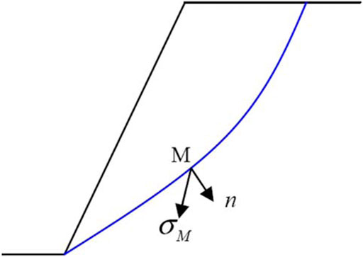
FIGURE 1. Sketch of a simple slope.
When the slope is about to slide, it can only slide along the potential slip surface because of the restriction of bedrock. Assuming the global sliding direction is d, the displacement of the slope can be expressed as Eq. 2.
Therefore, when the displacement of the slope is ds, the change of potential energy can be given by:
Then, the first-order variation can be written as
Eq. 4 can also be considered as:
where
Finally, the global sliding angle
where
2.2 The Safety Factor Based on Strength Reduction Technique
Because of the strength decrease of the soil, the potential sliding body can gradually fail from the normal stress state, as shown in Figure 2. At the critical stress state, the total resisting and driving forces should be equal along the global sliding direction, and the force equilibrium equation can be established by Eq. 7.
where
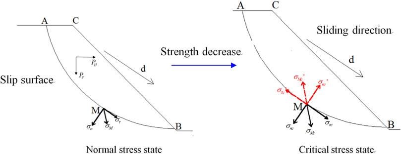
FIGURE 2. Sketch of the stress state from normal to critical state.
For the resisting stress on the slip surface, the Mohr–Coulomb yield criterion was utilized to determine the shear strength of the soil, which can be expressed as Eq. 8
where
Furthermore, the loads applied on the slope remain unchanged during the evolution process from the normal to the critical state, then, the assumption was made that the normal stress remains constant during the evolution process from the normal to the critical state of the slope.
Hence, the resisting forces along the slip surface along the sliding direction can be simplified as Eq. 9.
where
At the normal state of the slope, the macroscopic forces applied on the sliding body and micro forces along the slip surface should be equal to Eq. 10.
where
Because of being considered invariable during the evolution process from the normal state to the critical state of the slope for macroscopic forces, the driving force remains constant for the potential sliding body, which can be expressed as Eq. 11.
Connecting Eqs 7–11, the force equilibrium equation can be simplified as
That is,
Further simplification can be made as Eq. 14:
As an invariable along the slip surface, the safety factor can be finally expressed as:
Eq. 15 demonstrates that the resisting and driving shear stresses have an effect on the FS when the force equilibrium of a slope is considered along the sliding direction. Moreover, the safety factor (Eq. 15) can be directly obtained by integrals along the slip surface rather than iterative calculation, which is required in the LEM and SRM in computing the FS.
3 A Real-Coded Genetic Algorithm
3.1 Structure of the Real-Coded Genetic Algorithm
At first, the initial population should be generated based on the geometrically feasible requirements of the individual, then, the corresponding fitness of each individual is also computed. After crossover, mutation, and selection operation to this population based on modifications to previous studies on the genetic algorithm, the next generation can be obtained as follows:
1) The parents are selected to be crossed to generate the offspring as the candidate of the next generation.
2) Meanwhile, the mutation is also operated on the same parents and the generated offspring can still be considered as the candidate for the next generation.
3) The offspring generated previously by the crossover and mutation operation are combined with the parents as the total candidates of the next generation.
4) Using the selection operation, the total candidates are selected to constitute the next generation including a specified number of individuals.
The aforementioned routine process is repeated until the requirement of convergence or a given number of generations is met. A real-coded GA for specific slope stability problems is explained in the following sections in detail.
3.2 Geometrically Feasible Individuals of Slip Surface
According to previous studies on encoding the slip surface using polygons with N nodes denoted as Vi (i = 1 … … N), the kinematically feasible, upward-concave, trail slip surface is also taken into account, which can be completely defined by the coordinates of its nodes from the bottom to top. First, the extreme nodes (i = 1 or i = N) are randomly generated lying within specific intervals on the slope boundary. Then, similarly, the interior nodes must lie within an allowable search domain restricted by specific requirements of the feasible and upward-concave slip surface.
Figure 3 shows a feasible slip surface with N = 6 nodes from bottom to top, and the top to bottom generation has a similar process with obvious changes of nodes, which is not presented in detail in this study. As shown in Figure 3, the feasible slip surface with six nodes can be generated by fulfilling the following geometrical and kinematical compatibility constraints.
1) The extreme nodes V1 and V6 randomly located within their allowable intervals using a uniform probability distribution on the slope boundary have to be constrained by their corresponding lower and upper intervals, (V1a V1b) and (V6a V6b) (Figure 3).
2) For the interior nodes, the parallel and equidistant auxiliary lines perpendicular to V1VN (Li in Figure 3) are used to produce feasible intervals for these interior nodes. Take the node V3 for example, a feasible interval can be defined by the lower (V3a) from the intersection of L3 with the V1V6 segment and upper extreme (V3b) from the intersection of L3 and the line V1V2. In terms of V4 and V5, the aforementioned procedure can be repeated to produce their feasible intervals on the corresponding lines L4 and L5. For the interior node V2, the soil mechanics can be used to estimate the slope toe angle to determine the upper extreme V2b except the lower extreme V2a from the intersection of L2 with the V1V6 segment (Rafael and Rafael, 2015).
3) Once the feasible intervals are defined, the nodes can be randomly located within the intervals using a uniform probability distribution.
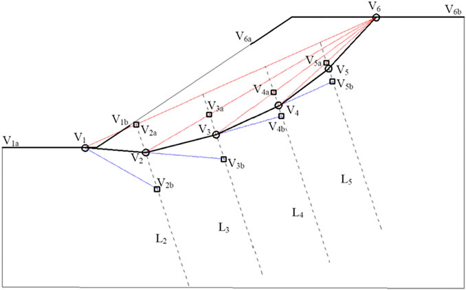
FIGURE 3. Generating process of a feasible slip surface of the initial population.
A feasible slip surface within the slope can be generated through the procedure mentioned previously, then, the initial population with certain individuals can be produced by repeating this procedure.
3.3 Selection Schemes
For the fitness of an individual of the population, the factor of safety (FS) can be naturally defined as the fitness of this individual. The critical slip surface of the slope we are trying to search corresponds to the global minimum FS within the slope, that is to say, the lower the FS of a slip surface is, the better it will be as the search target. The FS can be computed by the vector sum method in Section 3, therefore, the fitness of each individual can be determined as the basis of the selection schemes.
According to the fitness ranking (i.e., the individual can be ranked with a fitness from low to high), the selecting probability of an individual is computed by Eq. 16
where
3.4 Crossover Operators
Based on previous studies on GA operators to work with the slip surface, the heuristic and arithmetic crossover operators are used in this study.
Before this crossover operator is performed, two parents must be selected with a specified probability (rcrs). Given two feasible slip surfaces, Si and Sj, with factors of safety FS (Si)
where
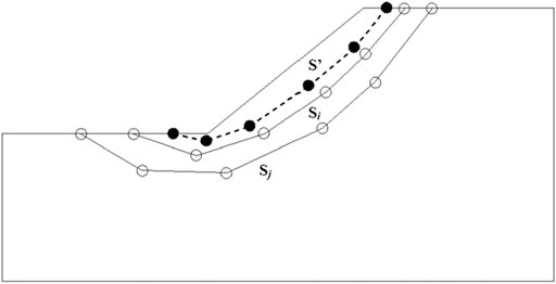
FIGURE 4. Sketch of the heuristic crossover operator.
Figure 5 shows the description of the arithmetic crossover operator, and two auxiliary polygonals, S′ and S″, can be produced by the given two parents, Si and Sj, as the offspring (Eqs 18, 19).
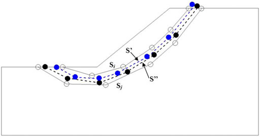
FIGURE 5. Sketch of the arithmetic crossover operator.
Similarly, the offsprings S′ and S″ also need to be individually tested through geometrical constraints described in Section 4.2, and if they are valid, they will be taken as the candidateS of the next generation. If no valid offspring is produced after a user-defined number of trails, the arithmetic operation of the parents, S′ and S″, returns no offspring.
3.5 Mutation Operators
Based on the custom mutation operators, four types are mainly used in this study, that is, uniform mutation, non-uniform mutation of single nodes, total non-uniform mutation, and extreme vertices mutation.
3.5.1 Uniform and Non-Uniform Mutation of a Single Node
For uniform and non-uniform mutations of a single node, there is a little difference between the interior node and extreme node. Figure 6 shows the mutation procedure on an interior node
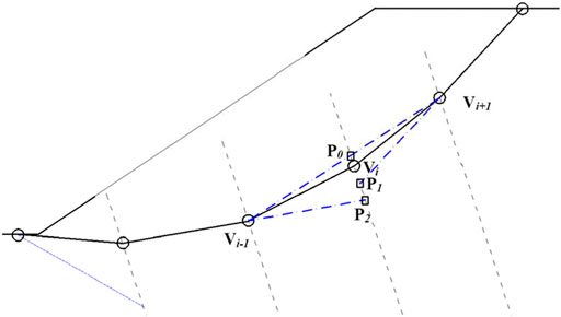
FIGURE 6. Sketch of uniform and non-uniform mutations of interior nodes.
For the extreme node, the feasible interval can be similarly obtained with a slight difference for interior nodes. Take the Vn for example, the feasible interval [PN0 or PN1] can be obtained as follows (Figure 7): PN0 is computed at the intersection between the slope boundary and a line traced from Vn-1 with a user-defined angle considering Rankine’s limit state (Li et al., 2010; Rafael and Rafael, 2015), whereas PN1 results as the intersection between the extension of the Vn-1Vn-2 segment and the slope boundary. If PN0 or PN1 lies outside the allowable extreme interval, it should be moved to the nearest interval extreme. The other extreme node V1 has a similar procedure and will not be discussed here.
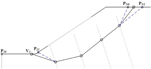
FIGURE 7. Sketch of uniform and non-uniform mutations of extreme nodes.
Using the feasible interval for all the nodes, the mutation can be operated. For uniform mutation of a single node, the mutated node
3.5.2 Total Non-Uniform Mutation and Extreme Vertices Mutation
The non-uniform mutation operator (Section 3.5.1) is applied to all nodes of a slip surface randomly selected from the population.
For extreme vertices mutation, the extreme nodes are mutated and the procedure is as follows: first, a valid individual (slip surface) is selected from the population, and the extreme nodes are mutated based on the procedure mentioned previously (Section 3.5.1). Then, the interior nodes will be newly generated using the new positions of both extreme nodes and the generation procedure in Section 3.2. Finally, a new slip surface will be produced as the candidate for the offspring.
In addition, a user-defined number of trails for each mutation operator is defined, and just like the crossover operation, if no valid offspring is produced after a user-defined number of trails, it will return no offspring.
3.6 Search Process
According to the description in Section 3, the search process of the real-coded GA to locate the critical slip surface is shown in Figure 8.
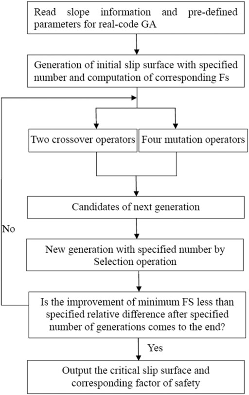
FIGURE 8. Search process of the critical slip surface using the real-code GA.
4 Application
To verify the reliability of the proposed approach, two examples are investigated from the literature and the results are compared with those in the literature. According to the theory of the vector sum method in Section 2, the finite element technique is used to obtain the stress field of the slope composed of elasto-plastic materials. The ideal elasto-plastic constitutive model, Mohr–Coulomb yield criterion, and non-associated flow rule are used in the elasto-plastic finite element analysis. As we know, the Gaussian integration points are used to integrate the stiffness matrix in the finite element analysis, and the discontinuous stresses with low accuracy at the boundary of elements are computed by the direct calculation of the stress integral. This study adopts the global stress smoothing technique to overcome the low accuracy deficiency. The stress at any position within an element can be calculated by
where n is the number of nodes of the element,
For the real-coded GA, many parameters, that is, the number of vertices Nvts defining the slip surface, the number of slip surfaces Mslip, probability of the crossover operator rcrs, probability of the mutation operator rmut, minimum number of generations Mterm before termination of search is allowed, and specified relative difference
4.1 Example 1
This example analyzes a homogenous benchmark slope organized by ACADS (Chen, 2003), and the standard FS of the slope is 1.0, that is, the slope is a critical slope.
These material properties of the homogenous slope are shown in Table 1. For computing conditions, the elastic model is adopted because this example is a critical slope, for which the standard FS is 1.00. For boundary conditions, the bottom is fixed and the lateral boundaries are normally restricted. The size of the slope is shown in Figure 9 and the calculating model of the finite element analysis is shown in Figure 10, and the total element number is 636.
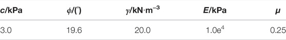
TABLE 1. Parameters of the material.
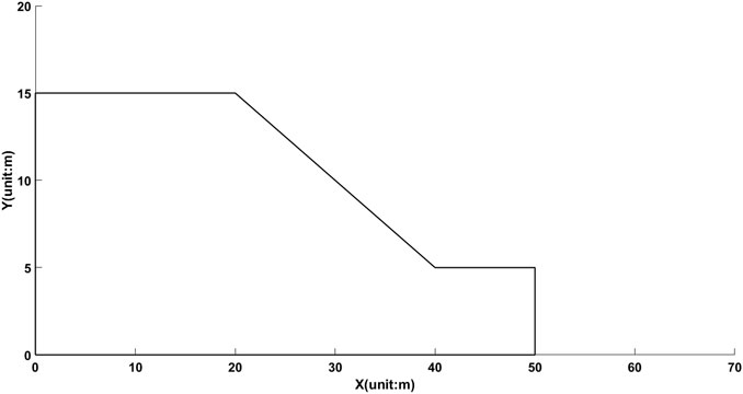
FIGURE 9. Geometry of the slope.
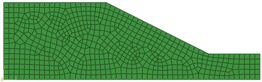
FIGURE 10. Calculating model of the finite element analysis.
The critical slip surface of this example can be searched using the real-code GA in Section 3 and the vector sum method in Section 2. Figure 11 shows the evolution with the number of generations using the real-code GA, of the minimum Fs with the vector sum method, which demonstrates the search process of the GA. Figure 12 shows the geometry and locations of the critical slip surfaces using the proposed approach and rigorous Morgenstern–Price method for comparison. From Figure 11 and Figure 12, it can be seen that either the location of the critical slip surface or corresponding minimum FS is in good agreement with the results obtained with the rigorous Morgenstern–Price method by the commercial software Geo-slope. Moreover, for this example, the minimum Fs by the proposed method or M–P method is almost equal to 1.0, which revealed that the vector sum method can reliably assess this example using this real-code GA.
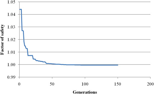
FIGURE 11. Evolution of Fs with the number of generations for example 1.
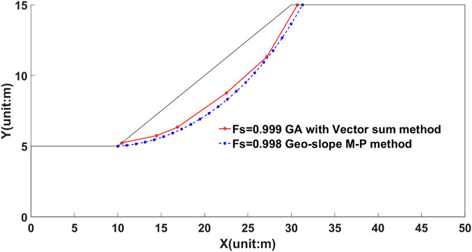
FIGURE 12. Locations of critical slip surfaces and corresponding Fs for example 1.
4.2 Example 2
This example is also initially organized by ACADS [Chen, 2003; Giam and Donald, 1989;], and used to test the ability of the proposed procedure for a non-circle slip surface. This slope includes a weak layer located between two strong layers, which is shown is Figure 13. Table 2 presents the properties of two types of soil layers. The factor of safety published by ACADS was equal to 1.26 for the specified slip surface, and for the critical slip surface, the FOS was organized to be 1.24. For boundary conditions, it is similar to that in example 1, that is, the bottom is fixed and the lateral boundaries are normally restricted.
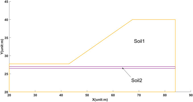
FIGURE 13. Profile of the slope for example 2.
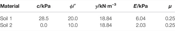
TABLE 2. Parameters of the material for example.2.
Moreover, this case was also studied with different optimization algorithms (Gandomi et al., 2017). Figure 14 shows the locations of critical slip surfaces and the corresponding FS by different optimization approaches, in which BBO means biogeography-based optimization and DE stands for differential evolution algorithm. From this figure, the exits of the critical slip surfaces with different approachs are almost located near the slope toe, and the entrances are located in a little different place on the top boundary of the slope. For the minimum FS, FS = 1.275, 1.214, 1.221, and 1.339, is obtained by GA with the vector sum method, DE with the M–P method, BBO with the M–P method, and GA with the M–P method, respectively. Except for FS = 1.339, the rest are consistent with the standard answer 1.24 organized by ACADS for this example. Figure 15 demonstrates the evolution process with the generations of the minimum FS, in which the global minimum FS can be obtained through almost 60 generations in the proposed GA (Figure 15).
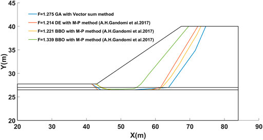
FIGURE 14. Locations of critical slip surfaces and corresponding Fs for example 2.
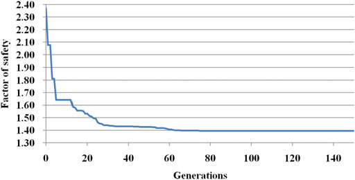
FIGURE 15. Evolution of Fs with the number of generations for example 2.
5 Discussions
1) Just like the conclusions of high efficiency to locate the critical slip surface for the real-coded GA reported in the literature (Sun et al., 2008; Sabhahit and Rao, 2011; Richard and Sitar, 2012; Rafael and Rafael, 2015), the real-coded GA presented in this study actually exhibits an excellent ability to find the critical slip surface for these complex slopes. From comparing the results of two examples with those reported in the literature, the vector sum method proposed in this study is verified to be reliable to assess slope-stability problems. Over traditional methods, that is, the limit equilibrium method and strength reduction technique, the vector sum method emphasizes the direction of the force and the global sliding direction of the slope, which brings new insights into the way we assess the slope problem. More importantly, this proposed method can not only provide the global sliding direction of the slope determined by rigorous theory but also directly compute the safety factor by force equilibrium of the sliding body on the basis of the stress state of the slope, which is also helpful to evaluate the slope stability under dynamic loads or some other complex loads. At present, the vector sum method still has a long distance to go for approval by researchers and engineers, but it explores a new approach to treat slope problems from other perspectives over traditional approaches.
2) Merely from the viewpoint of the formula to calculate the safety factor, the computing formula by force equilibrium (Eq. 15) of the proposed method is just the vector expression of the formula recognized as an important supplement for the theory of slope-stability analysis over the traditional LEM and SRM. The slope-stability problem is essentially a nondeterministic polynomial-time complete problem, and one approach cannot completely replace the other because of the approximation feature of all approaches to slope-stability problems (Tang et al., 2015). To be honest, for 2D slope-stability problems, it is not difficult to accurately evaluate the stability of the slope using either commercial software Geo-slope with the LEM or other with the SRM. However, in 3D complex problems, it is not easy to reasonably assess the slope problem, especial for dynamic slope problems. The proposed approach in this study also has high efficiency for 3D slope-stability problems with complex conditions as long as the stress state of the slope can be rationally obtained by numerical simulation.
6 Conclusion
1) Based on the popular strength reduction definition in the slope stability analysis, the vector sum method was further studied and the safety factor was deduced on the basis of the force equilibrium equation along the global sliding direction.
2) The proposed approach was proved to be reliable in assessing the slope stability by comparing the locations of critical slip surfaces and corresponding FS of examples with those obtained using the M–P method and other optimization algorithms in the literature.
3) For the real-coded GA, though only six vertices are considered in this study for finding the critical slip surface, it still exhibits high efficiency on locating the critical slip surface for two examples.
Data Availability Statement
The original contributions presented in the study are included in the article/Supplementary Material; further inquiries can be directed to the corresponding author.
Author Contributions
MG contributed to conception and design of the study. JL organized the database. XD performed the statistical analysis. MG wrote the first draft of the manuscript.
Funding
This study was funded by the National Science Foundation of China under Grant No. 51674239.
Conflict of Interest
The authors declare that the research was conducted in the absence of any commercial or financial relationships that could be construed as a potential conflict of interest.
Publisher’s Note
All claims expressed in this article are solely those of the authors and do not necessarily represent those of their affiliated organizations, or those of the publisher, the editors, and the reviewers. Any product that may be evaluated in this article, or claim that may be made by its manufacturer, is not guaranteed or endorsed by the publisher.
Acknowledgments
The authors gratefully acknowledge the financial support of the National Science Foundation of China under Grant No. 51674239.
References
Chen, Z. Y. (2003). Earth Slope Stability Analyses—Theory, Method and Programs. Beijing: China Water Power Press.
Cheng, Y. M., Lansivaara, T., and Wei, W. B. (2007). Two-dimensional Slope Stability Analysis by Limit Equilibrium and Strength Reduction Methods. Comput. Geotechnics 34, 137–150. doi:10.1016/j.compgeo.2006.10.011
Duncan, J. M. (1996). State of the Art: Limit Equilibrium and Finite-Element Analysis of Slopes. J. Geotechnical Eng. 122 (7), 577–596. doi:10.1061/(asce)0733-9410(1996)122:7(577)
Fu, X., Sheng, Q., Zhang, Y., Chen, J., Zhang, S., and Zhang, Z. (2017). Computation of the Safety Factor for Slope Stability Using Discontinuous Deformation Analysis and the Vector Sum Method. Comput. geotechnics 92, 68–76. doi:10.1016/j.compgeo.2017.07.026
Gandomi, A. H., Kashani, A. R., Mousavi, M., and Jalalvandi, M. (2017). Slope Stability Analysis Using Evolutionary Optimization Techniques. Int. J. Numer. Anal. Methods geomechanics 41, 151–264. doi:10.1002/nag.2554
Ge, X. R. (2008). Deformation Control Law of Rock Fatigue Failure,real-Time X-ray CT Scan of Geotechnical Testing, and New Method of Stability Analysis of Slopes and Dam Foundations. Chin. J. Geotechnical Eng. 30 (1), 1–20.
Giam, P. S. K., and Donald, I. B. (1989). Example Problems for Testing Soil Slope Stability Programs. Civil Eng. Res. 8, 1989.
Guo, M. W., Li, C. G., Wang, S. L., Yin, S. D., Liu, S. J., and Ge, X. R. (2019). Vector-Sum Method for 2D Slope Stability Analysis Considering Vector Characteristics of Force. Int. J. geomechanics 19 (6), 1436. doi:10.1061/(ASCE)GM.1943-5622.0001436
Hamdhan, I. N., and Schweiger, H. F. (2013). Finite Element Method-Based Analysis of an Unsaturated Soil Slope Subjected to Rainfall Infiltration. Int. J. Geomech. 13 (5), 653–658. doi:10.1061/(asce)gm.1943-5622.0000239
Huang, C.-C., and Tsai, C.-C. (2000). New Method for 3D and Asymmetrical Slope Stability Analysis. J. Geotech. Geoenviron. Eng. 126 (10), 917–927. doi:10.1061/(asce)1090-0241(2000)126:10(917)
Kim, J. Y., and Lee, S. R. (1997). An Improved Search Strategy for the Critical Slip Surface Using Finite Element Stress fields. Comput. Geotechnics 21 (4), 295–313. doi:10.1016/s0266-352x(97)00027-x
Li, Y.-C., ChenZhan Tony, Y.-M. L. T., Zhan, T. L. T., Ling, D.-S., and Cleall, P. J. (2010). An Efficient Approach for Locating the Critical Slip Surface in Slope Stability Analyses Using a Real-Coded Genetic Algorithm. Can. Geotech. J. 47 (7), 806–820. doi:10.1139/t09-124
Liu, G., Zhuang, X., and Cui, Z. (2017). Three-dimensional Slope Stability Analysis Using Independent Cover Based Numerical Manifold and Vector Method. Eng. Geology. 225, 83–95. doi:10.1016/j.enggeo.2017.02.022
Rafael, J. P., and Rafael, J. (2015). A Genetic Algorithm for Slope Stability Analyses with Concave Slip Surfaces Using Custom Operators. Eng. Optimization 47 (4), 453–472. doi:10.1080/0305215X.2014.895339
Richard, O. C., and Sitar, N. (2012). bSLOPE A General Limit Equilibrium Slope Stability Analysis Code for iOSGeotechnicalEngineering Report No. UCB/GT/12-01 2012. Berkeley, CA: Department of Civil and Environmental Engineering, University ofCalifornia.
Sabhahit, N., and Rao, A. (2011). Genetic Algorithms in Stability Analysis of Non-homogeneous Slopes. Int. J. Geotechnical Eng. 5 (1), 33–44. doi:10.3328/ijge.2011.05.01.33-44
Shen, J., and Karakus, M. (2014). Three-dimensional Numerical Analysis for Rock Slope Stability Using Shear Strength Reduction Method. Can. Geotech. J. 51, 164–172. doi:10.1139/cgj-2013-0191
Sun, J., Li, J., and Liu, Q. (2008). Search for Critical Slip Surface in Slope Stability Analysis by Spline-Based GA Method. J. Geotech. Geoenviron. Eng. 134 (2), 252–256. doi:10.1061/(asce)1090-0241(2008)134:2(252)
Tang, H., Liu, X., Xiong, C., Wang, Z., and Ez Eldin, M. A. M. (2015). Proof of Nondeterministic Polynomial-Time Complete Problem for Soil Slope-Stability Evaluation. Int. J. Geomechanics 16 (5), 595. doi:10.1061/%28ASCE%29GM.1943-5622.0000595
Zheng, H., Tham, L. G., and Liu, D. (2006). On Two Definitions of the Factor of Safety Commonly Used in the Finite Element Slope Stability Analysis. Comput. Geotechnics 33, 188–195. doi:10.1016/j.compgeo.2006.03.007
Keywords: slope stability, vector sum method, genetic algorithm, critical slip surface, safety factor
Citation: Guo M, Li J and Dong X (2022) Determining the Critical Slip Surface of Slope by Vector Sum Method Based on Strength Reduction Definition. Front. Earth Sci. 10:865017. doi: 10.3389/feart.2022.865017
Received: 29 January 2022; Accepted: 31 March 2022;
Published: 29 April 2022.
Edited by:
Fei Meng, Swinburne University of Technology, AustraliaReviewed by:
Ashok Kumar Gupta, Jaypee University of Information Technology, IndiaYunfeng Ge, China University of Geosciences, China
Copyright © 2022 Guo, Li and Dong. This is an open-access article distributed under the terms of the Creative Commons Attribution License (CC BY). The use, distribution or reproduction in other forums is permitted, provided the original author(s) and the copyright owner(s) are credited and that the original publication in this journal is cited, in accordance with accepted academic practice. No use, distribution or reproduction is permitted which does not comply with these terms.
*Correspondence: Mingwei Guo, bXdndW9Ad2hyc20uYWMuY24=