Deciphering the Properties of Different Arctic Ice Types During the Growth Phase of MOSAiC: Implications for Future Studies on Gas Pathways

The increased fraction of first year ice (FYI) at the expense of old ice (second-year ice (SYI) and multi-year ice (MYI)) likely affects the permeability of the Arctic ice cover. This in turn influences the pathways of gases circulating therein and the exchange at interfaces with the atmosphere and ocean. We present sea ice temperature and salinity time series from different ice types relevant to temporal development of sea ice permeability and brine drainage efficiency from freeze-up in October to the onset of spring warming in May. Our study is based on a dataset collected during the Multidisciplinary drifting Observatory for the Study of Arctic Climate (MOSAiC) Expedition in 2019 and 2020. These physical properties were used to derive sea ice permeability and Rayleigh numbers. The main sites included FYI and SYI. The latter was composed of an upper layer of residual ice that had desalinated but survived the previous summer melt and became SYI. Below this ice a layer of new first-year ice formed. As the layer of new first-year ice has no direct contact with the atmosphere, we call it insulated first-year ice (IFYI). The residual/SYI-layer also contained refrozen melt ponds in some areas. During the freezing season, the residual/SYI-layer was consistently impermeable, acting as barrier for gas exchange between the atmosphere and ocean. While both FYI and SYI temperatures responded similarly to atmospheric warming events, SYI was more resilient to brine volume fraction changes because of its low salinity ($<$ 2). Furthermore, later bottom ice growth during spring warming was observed for SYI in comparison to FYI. The projected increase in the fraction of more permeable FYI in autumn and spring in the coming decades may favor gas exchange at the atmosphere-ice interface when sea ice acts as a source relative to the atmosphere. While the areal extent of old ice is decreasing, so is its thickness at the onset of freeze-up. Our study sets the foundation for studies on gas dynamics within the ice column and the gas exchange at both ice interfaces, i.e. with the atmosphere and the ocean.

1 Introduction

Arctic sea ice has a major impact on global climate and the ongoing sea ice retreat induces intense shifts at the atmosphere-ocean interface, e.g. air-sea gas fluxes. Summer sea ice extent has decreased since the 1970s and has accelerated since 2000 (Comiso et al., 2008). As a consequence of the diminishing summer sea ice extent, the relative proportion of younger and thinner sea ice is increasing. From 1984–2017, the areal fraction of first-year ice (FYI) in the Arctic Ocean increased from approximately 40% to 70% (Tschudi et al., 2020), while the areal fraction of thicker old ice decreased. For instance, the fraction of winter sea ice cover older than 5 years decreased from 30% in 1984 to 2% in 2018 (Stroeve and Notz, 2018). Interestingly, the fraction of second-year ice (SYI) aged 1–2 years slightly increased from about 12% to 17% over the same period (Tschudi et al., 2020). Despite the slightly increasing areal extent of SYI, its thickness at the onset of freeze-up is decreasing, leading to increased winter ice growth beneath (Petty et al., 2018). However, this might be extremely sensitive to snow depth on the sea ice, as SYI likely accumulates more snow which affects ice growth (Merkouriadi et al., 2017). Seasonal sea ice, or FYI, is more susceptible to phase changes in the entire ice slab than older multi-year sea ice (MYI) when it warms (Vancoppenolle et al., 2005). The shift to more seasonal ice affects the overall physical properties of the Arctic ice pack, and therefore likely also the ice permeability and potential gas pathways within the ice (Verdugo et al., 2020).

While globally-representative monthly rates of change of atmospheric carbon dioxide and methane concentrations are correlated with sea ice dynamics, it is still unclear if sea ice acts as an active driver or is simply a proxy for alternative drivers (Hambler and Henderson, 2022). Furthermore, sea ice has been shown to be a source of ozone-depleting compounds in summer, as well as in winter (Granfors et al., 2013; Abrahamsson et al., 2018). To gain insights into potential underlying mechanisms, we designed an integrative biogeochemistry study carried out during the MOSAiC drift expedition, tracing the evolution of the sea ice’s permeability (derived from temperature and salinity) and the development and modification of climate-relevant gas (CRG) pathways in various ice types from autumn freeze-up (October) to spring warming (May). These CRGs include methane, halocarbons, nitrous oxide, dimethylsulfide, and dimethylsulfoxide. An overview of Team BioGeoChemistry (BGC) activities is summarized in a manuscript prepared by E. Damm et al.

MOSAiC was an international transpolar drift expedition in which the German icebreaker RV Polarstern anchored into an ice floe to gain new insights into Arctic climate over a full annual cycle. In October 2019, RV Polarstern moored to an ice floe in the Siberian sector of the Arctic at 85° N and 137° E to begin the drift towards the North Pole and the Fram Strait via the Transpolar Drift Stream. Overview papers describing the activities of the ice physics, physical oceanography, and atmospheric science teams are available from Nicolaus et al. (2022), Rabe et al. (2022), and Shupe et al. (2022), respectively. In our paper, we present baseline information to understand the temporal development of sea ice permeability for different ice types during the ice growth season inferred from temperature and salinity measurements. Our goal was to estimate the variations of the brine content in the ice column during the winter/early spring season and to establish time series of brine volume fraction and Rayleigh number as preconditions to interpret how CRG circulation evolves from the onset of sea ice growth to spring warming. The data presented in this paper were collected during the first three legs of the expedition, because all the ice coring activities took place on the same ice floe and the ice surface melt season had not yet started. The end dates of legs 1, 2, and 3 were 13 December, 24 February, and 4 June, respectively. Data collection during leg 3 stopped on 9 May. At the end of leg 3, RV Polarstern left the floe (approximately 400 km north of Svalbard) and travelled to Svalbard for supplies and personnel exchange. The RV Polarstern drift trajectory is shown in Figure 1.

FIGURE 1

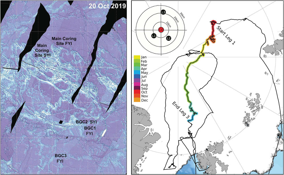
FIGURE 1. Left panel: Central Observatory map of 20 October 2019 generated from helicopter laser scanner surveys (credit: Stefan Hendricks). Brighter shades of blue indicate larger surface elevation, i.e. pressure ridges can be seen as well. The main coring and BioGeoChemistry (BGC) FYI and SYI sites were on the same floe from late October 2019 to early May 2020, but their relative positions changed due to local ice movements. Right panel: The RV Polarstern MOSAiC track is shown by the black line and the drift trajectory from legs 1 to 3 by the coloured segments, modified from Nicolaus et al. (2022). The background shows the sea ice extent for March 2020. In the top left of the panel, the position of the Central Observatory (CO) in the red circle relative to the L sites of the Distributed Network for 22 October 2019 is shown and modified from Krumpen and Sokolov (2020).

To study brine dynamics of young sea ice at the ice/water interface, Notz and Worster (2008) showed in situ measurements of sea ice salinity to capture desalination at specific ice depths on a better than hourly basis over a few days in March. Using the mushy-layer approach for interpretation, they show that brine gravity drainage occurs continuously in the lower centimetres of activity growing sea ice. Newly formed sea ice also loses salt through salt segregation at the ice/ocean interface. More specifically, salts are rejected from growing ice crystals since the crystal lattice can only incorporate a limited amount of salt. The amount of salt incorporated into growing ice or the “initial entrapment” is positively correlated with the ice growth rate (Eicken, 1998). The rejected salts increase the seawater density at the ice/water boundary, triggering convection. Salt segregation is associated with the boundary-layer approach of convection, whereas brine gravity drainage is associated with the mushy-layer approach. Both modes play a role in sea ice salinity evolution as discussed in Middleton et al. (2016). The salinity for a specific ice depth that follows once brine drainage diminishes is referred to as the “stable salinity” (Nakawo and Sinha, 1981). The granular ice layer close to the top ice surface is often more saline than the underlying columnar ice, because it forms quickly and under turbulent sea conditions (Notz and Worster, 2008) and the bottom ice layer is more saline than the ice above because it is younger, which typically leads to a C-shaped salinity profile for FYI. The columnar sea ice near the ice surface is also more saline than the underlying columnar sea ice because it generally grows faster. Research by Johnston (2017) analyzed sea ice cores from fast and pack ice from the Canadian Archipelago (1980–2015), including FYI, SYI, and MYI. The study showed that the strength of SYI deteriorated 1 month after that of FYI in summer, because the SYI included a desalinated surface layer from the previous year. By desalination, we refer to drainage affecting the permeable ice fraction in the ice column, not just the brine release that occurs in the hours to days following new ice formation at the ice/ocean interface. Since the time series shown in this paper span from late October to early May, the ice surface melt season is not included. Therefore, salt loss in sea ice triggered by the flushing of melt water in summer is not represented in our time series.

Most time series studies of sea ice cores were carried out in regions of FYI, whereas old ice (SYI/MYI) has been investigated less. Pioneering work provided a landfast FYI time series in the Canadian Arctic from freeze-up to melt onset (Nakawo and Sinha, 1981), while Cox and Weeks (1988) compared numerical modelling results of FYI growth and field data to understand the evolution of sea ice properties. Time series of FYI in the growth and melt seasons have also been performed in Alaskan and Svalbard landfast ice (Oggier et al., 2020). Work by Granskog et al. (2017) compared FYI and SYI salinity and oxygen isotopic composition in drifting ice north of Svalbard but their data are limited to short time series on single floes over the January to June period.

As we partly deviate from basic definitions of sea ice nomenclature (WMO, 2014), we present some basic definitions and how they are used in this paper. FYI is sea ice that develops in a single growth season and is at least 30 cm thick. If FYI survives the summer melt season, it becomes residual ice. Starting on 1 January, residual ice transitions to SYI as defined by the World Meteorological Organization (WMO). For simplicity, we use SYI to describe both residual ice and SYI. In this paper, we consider the ice that grows underneath SYI during winter as a type of FYI. For biogeochemical studies in the Lincoln Sea, Lange et al. (2015) denoted this ice as “new ice.” The WMO defines new ice as a general term for any recently formed ice, irrespective of the conditions surrounding its formation. In our paper, we refer to ice growing beneath SYI as insulated first-year ice (IFYI), to highlight the importance of the SYI-layer’s thermal buffering capacity and low salinity, which directly impact CRG transport pathways. Additional snow accumulation would also contribute to the thermal buffering capacity of SYI sites. Rafted ice refers to any type of deformation resulting in an ice slab submerging below another.

A time series of ice cores is needed to dissect how SYI permeability differs from FYI over the course of the complete ice growth period. Further, quantifying the susceptibility of sea ice to brine gravity drainage with the Rayleigh number as used in previous biogeochemical studies such as Zhou et al. (2013), Crabeck et al. (2019), Gourdal et al. (2019), and Van der Linden et al. (2020) can lead to new insights on CRG pathways in sea ice. Drainage events transport CRG dissolved in the brine from the sea ice to the ocean (Damm et al., 2015), so the Rayleigh number hints at the relative onset of these events for different ice types. Brine drainage is a downward directed CRG pathway (e.g. Verdugo et al. (2020)), while upward directed CRG pathways in the entire ice column depend on bubble formation (e.g. Zhou et al., 2013; Tison et al., 2017; Crabeck et al., 2019). More importantly, one precondition for a sea-ice to air gas flux is bubble transport to the surface, which can only happen if the ice is permeable throughout the ice.

We hypothesize that FYI and SYI exhibit distinct differences in their temporal permeability evolution from late autumn to spring, with correspondingly different implications for brine release and gas dynamics within sea ice and at the interfaces with the atmosphere and ocean. While a plethora of sea ice core data exists for the spring to early autumn timeframe from previous field campaigns, FYI and SYI time series during the polar night are limited. Our study represents one of the first time series of FYI and SYI on the same ice floe for the entire ice growth period. For the first time, several co-incident polar night time series from spatially varying FYI and SYI types are presented. To investigate the inter-site spatial variability of the different ice types, we present more than one time series for both FYI and SYI. Ultimately, the aim is to improve the parameterization for various numerical biogeochemical models, furthering our understanding of CRG pathways in an Arctic Ocean with increasing FYI fraction in winter. With an improved process understanding of CRG cycling in the Arctic Ocean, we can ultimately predict the seasonal switches between the upward and downward directed CRG pathways as the Arctic Ocean warms and the fraction of seasonal ice increases.

2 Sampling Sites

The oldest part of the MOSAiC Central Observatory (CO) originated from the New Siberian Islands, where the ice formed during a polynya event in December 2018 (Krumpen et al., 2020). From a biogeochemical perspective, understanding the origin of ice floes is important, because it has been shown that the Transpolar Drift Stream transports methane trapped in sea ice from shallow shelf regions to the central Arctic Ocean (Damm et al., 2018). We investigated multiple locations representing FYI and SYI, both in the CO and the Distributed Network (DN) (Figure 1). The BioGeoChemistry (BGC) sites were identified as BGC1 (FYI), BGC3 (FYI), and BGC2 (SYI), respectively. There was also a main coring site (MCS) for FYI and SYI that multiple teams jointly worked on. These are denoted as MCS-FYI and MCS-SYI. BGC sites 1–3 are specific sites for studies of CRG circulation and at the MCS, BGC studies were conducted in addition to the detailed ice physics studies (Nicolaus et al., 2022).

2.1 Sites in the Central Observatory

Site BGC1 was a FYI area that developed in open seawater (presumably in October 2019) surrounded by residual sea ice (Figure 1). Site BGC2 was far more heterogeneous and included SYI, SYI with freshwater pockets, as well as ridged and rafted ice. The water pockets were presumably from melt ponds that had not completely refrozen. For the autumn to spring time series, only the SYI area without water pockets was repeatedly investigated. Site BGC3 contained FYI with localized rafted ice. At MCS-FYI, rafted areas were encountered in March and April 2020 and at MCS-SYI, the ice contained a strongly desalinated upper layer. The MCS was located suitably far away from the ship to not be affected by the RV Polarstern lights during polar night (Nicolaus et al., 2022).

2.2 Distributed Network

The DN consisted of ice floes of similar age as the central floe (Krumpen et al., 2020). We investigated ice at the DN sites L1, L2, and L3, which are described in an overview manuscript prepared by B. Rabe et al. At all three sites (5–10 October 2019), the level ice was approximately 0.35 m thick and classified as residual ice (eventually becoming SYI) (Krumpen and Sokolov, 2020). We collected 16 cores in October 2019, including rafted ice where the mean ice thicknesses were 3.0 m at L2 and 1.3 m at L3. We repeated coring at the FYI and SYI L1 and L2 sites until April 2020.

3 Methods

3.1 Ice Coring

The reader is referred to Nicolaus et al. (2022) for a comprehensive summary of the ice coring methodology at the main coring sites, which was more comprehensive because it accounted for the needs of multiple teams and targeted co-incident work on sea ice physical and biological processes. Here we present a brief ice coring methodology used for the data. Sea ice cores were collected with a Kovacs Mark II 9 cm diameter corer (Kovacs Enterprises, Inc.). Normally, three to four ice cores were collected at each site. In addition, vertical snow sampling was carried out for halocarbon analyses, and thus snow depth data is available. On the first leg of the expedition, ice cores were taken on an almost weekly basis, but afterwards, the coring dates were less frequent, due to the weather conditions and sea ice dynamics hampering access to the coring sites. In each case, the first core was used for temperature measurements while on all BGC-related ice cores, the salinity was measured. Each collected ice core was used for specific measurements of trace gases.

To measure ice temperatures on leg 1 at the BGC sites, about 4.5 cm deep holes were drilled into the core at 5 cm intervals starting from the snow/ice interface. On legs 2 and 3, holes were drilled at 2.5, 7.5, and 15 cm from the top and then at 10 cm intervals. For MCS cores from legs 1–3, holes were drilled at 2.5 cm from the top and 2.5 cm from the bottom of the core. Holes were then drilled at 10 cm intervals from both the top and bottom of the core until the core midpoint. Occasionally, temperature locations were adapted for breaks, gaps, or brittle segments in the cores. The temperatures were measured by a digital thermometer within minutes after the cores were retrieved. For the ice bottom temperature, the temperature probe was placed directly into the core bottom. To complete the sea ice thermal regime, temperatures were also measured in the air, as well as at the air/snow and snow/ice boundaries. The ice cores were placed into pre-labelled plastic sleeves sealed at the bottom end. At the top, the plastic sleeves were secured with multiple zip-ties. Since the cores in this study were not sectioned in the field, we acknowledge that some brine might have been lost. Losing brine results in an underestimation of sea ice permeability derived from temperature and salinity data. The ice cores were then transported to RV Polarstern and stored in a −20°C freezer. Each of the cores was sub-sampled, melted at room temperature, and processed for salinity within one or 2 days. The practical salinity was estimated by measuring the electrical conductivity and temperature of the melted samples using a WTW Cond 3151 salinometer equipped with the Tetra-Con 325 four-electrode conductivity cell. The absolute salinity [g/kg] is the amount of dissolved salts per mass of ice or solution after melting. The practical salinity [dimensionless] represents the salinity estimated from the electrical conductivity of the solution. For standard seawater composition, the absolute salinity is approximately equal to the practical salinity. In this paper, we present practical salinity.

3.2 Brine Volume Fractions

The brine volume fraction (BVF) was calculated from the temperature and salinity of each core sample. The fundamental unit of ice microstructure is an ice grain surrounded by brine and sometimes air voids. As the temperature and salinity of ice increase, the brine volume fraction increases. When the BVF exceeds 5% for columnar sea ice, the brine inclusions interconnect, and the ice is said to become permeable for brine movement (Golden et al., 2007). If the BVF is less than 5%, the ice is said to be impermeable. The ice core sectioning in the laboratory for BGC-related cores resulted in sample midpoints that did not always correspond to the ice depth associated with the temperature measurement. Therefore, ice temperatures were linearly interpolated between measurement depths and the interpolated values were extracted at each sample midpoint. If sample midpoints fell outside the interpolated temperature range, then the following rules were applied. If the length of an ice core exceeded the temperature core length, then the bottom ice temperature (normally equal to the seawater temperature) value was used for sample midpoints deeper than the maximum depth of the temperature core. Since the temperature core usually had a similar thickness to the adjacent cores (within 10 cm), we did not adjust the entire temperature profile for slightly different core lengths. If the snow/ice boundary temperature was not recorded and a sample midpoint was shallower than the uppermost ice temperature measurement, then the latter ice temperature was used. The temperature (T, in degree Celsius (°C)) assigned to the sample midpoint and the salinity of each melted ice sample were used to calculate the BVF. For −2.0°C $>T\ge$−30°C, the BVF was estimated according to Eq. 1 (Cox and Weeks, 1983). To calculate the sea ice density (ρ), the pure ice density as a function of temperature was first estimated from Fukusako (1990). The sea ice density equation considers temperature-dependent phase equilibrium relationships from Assur (1960) for brine salinity (S_b) and the ratio (k) of the mass of solid salts to the mass of salts in the brine. When implementing the sea ice density equation, we assumed no air volume. The BVF was calculated from Eq. 1, where F₁(T) = ρ_b S_b (1+k) and ρ_b is brine density. The brine salinity, density, and the amount of solid salts all vary as a function of temperature.

$BVF=\frac{\rho S}{F_1\left(T\right)}(1)$

The BVF estimation in Eq. 1 accounts for the eutectic points of different salts in seawater, meaning that some brine still exists below the eutectic temperature of the H₂O-NaCl phase equilibrium system. In the case of T ≥ −2.0°C, estimates for ρ and F₁(T) to calculate BVF were adjusted following Leppäranta and Manninen (1988) for warm ice conditions. These conditions only occurred in the ice column in early October 2019, at the ice bottom, as well as the interface of ice and water pockets.

3.3 Rayleigh Number

Since the BVF threshold of 5% is only a proxy indicating when brine channels are potentially interconnected, the Rayleigh number (Ra) is calculated to determine when brine gravity drainage can occur (Notz and Worster, 2009). The Ra is dimensionless, characterizes a fluid’s flow regime, and determines when convection occurs. The proposed critical Ra values that yield the onset of convection range between 2 and 10 in the literature. For experimental and field studies, Ra thresholds towards the lower end are typically used (Gourdal et al., 2019). The rationale behind this stems from the fact that critical Ra numbers occur transiently. Calculating a critical Ra depends on the physical properties and thus when ice cores are drilled. More specifically, the critical Ra might be missed if brine drainage occurs between ice coring dates. Secondly, brine loss upon core retrieval may result in a lower salinity than the in situ value (especially at the ice bottom) and consequently results in a lower Ra number. In Gourdal et al. (2019), the Ra number was used to delineate unstable gravity drainage and vertically stable phases for FYI in the Canadian Arctic during spring warming and summer melt. In their study, the authors found that dimethyl sulfide was transported from the ice bottom to the atmosphere during the vertically stable phase. In our paper, we employ the lower Ra threshold of 2 to interpret the relative onset of drainage events for different ice types between autumn and spring. The effective sea ice permeability, Π [m²], is a function of BVF and can be estimated from Eq. 2 (Freitag, 1999), where BVF_min is the minimum BVF between the ice depth in question and the ice bottom. The ice depth in question refers to the depth of an ice core sample, since an Ra is calculated for each sample interval. Therefore, a layer of low permeability can affect the propensity for brine gravity drainage in the entire ice column. The permeability is a variable in the Ra calculation shown in Eq. 3, where h [m] is the ice depth from the snow/ice surface to the ice/seawater interface, z [m] is the ice depth in question, β is the haline expansion coefficient of seawater, g is the acceleration due to gravity, ΔS_b is the salinity difference across (h-z) [ppt], κ is the thermal diffusivity for cold seawater, and μ is the dynamic viscosity constant of seawater extrapolated for the brine. The values for β, κ, and μ were taken from Gourdal et al. (2019) and all Ra parameter values are shown in Table 1. When calculating (h-z), we used the top of an ice sample as z and for ΔS_b, we used a constant seawater salinity of 32 ppt for simplicity. In the case of water pockets, we treat them as part of the ice column and maintain h as the ice depth from the snow/ice interface to the ice/seawater interface. The brine salinity was calculated following Notz and Worster (2009). Since Eq. 2 was derived for young ice, we acknowledge the limitations in estimating the Ra for FYI and SYI. Hence, the Ra is used as a relative indicator for the onset of drainage between the different sampling sites, but not as an absolute predictor of when it actually occurs.

$\mathrm{\Pi }=10^{-17}{\left[10^3\left(BV{F}_{\mathit{min}}\right)\right]}^{3.1}(2)$

$Ra=\frac{\left(h-z\right)g\beta \mathrm{\Delta }{S}_b\mathrm{\Pi }}{\kappa \mu }(3)$

TABLE 1

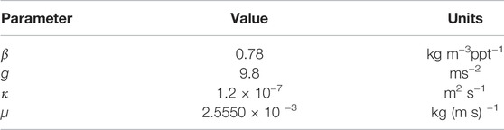
TABLE 1. Parameters for Rayleigh number calculation.

3.4 Time Series and Interpolation

To generate a time series of T, S, BVF, and Ra, we used the natural neighbor interpolation method in MATLAB. To generate smooth figures, temporal and vertical grid cells of 0.25 days and 10 cm were used in the mesh. The values were stored at sample midpoints and samples with no data were excluded. Physical property values at the same ice depth for adjacent ice cores on the same day were averaged prior to interpolation. To visualize water pocket evolution, values of 1 (water pocket exists) and 0 (no water pocket) were assigned for each sample. The water pocket indicators were also interpolated using the natural neighbor interpolation method and all mesh cells with a water pocket indicator above 0.5 were blanked out to approximate a water pocket’s expansion or contraction through time. For the presented time series, a seawater pocket was present at BGC3 in early November, but was not encountered the following coring week. This site likely consisted of two rafted FYI floes, which created the water pocket. Given the uncertainty, all the ice cores for BGC3 cores are included in the interpolation. We acknowledge that interpolating between large gaps in ice coring days does not show all short-term changes in the ice’s physical properties from autumn to spring, especially for temperature and BVF. However, the interpolations still show macro-trends in sea ice permeability and the impacts of isolated effects like warm air intrusions (WAI) in autumn. Since BGC3 has an ice temperature gap of more than 2 months, the interpolation for this site was divided into two segments. In each time series, snow thickness at the coring locations and air temperature trends are presented. The total number of ice cores with salinity profiles used in the interpolated graphics were 34 (BGC1), 37 (MCS-FYI), 19 (BGC3), 15 (BGC2), and 27 (MCS-SYI).

4 Results: Evolution of Sea Ice Permeability

4.1 Initial Conditions of the Central Observatory Compared to the Distributed Network

In Figure 2, we present the temperature, salinity, and BVF of sea ice upon the first site visit for the CO sites in comparison with the L sites in the DN. The highest salinities were observed for FYI, which showed C-shaped salinity profiles for BGC1 and MCS-FYI in late October. The FYI at BGC3 showed a more vertically uniform salinity profile, but the first site visit was in early November and the ice was observed to be rafted. The entire FYI slab was likely permeable from the ice surface down to the ice bottom during the first visit because the BVF was $\ge 5$% at all ice depths.

FIGURE 2

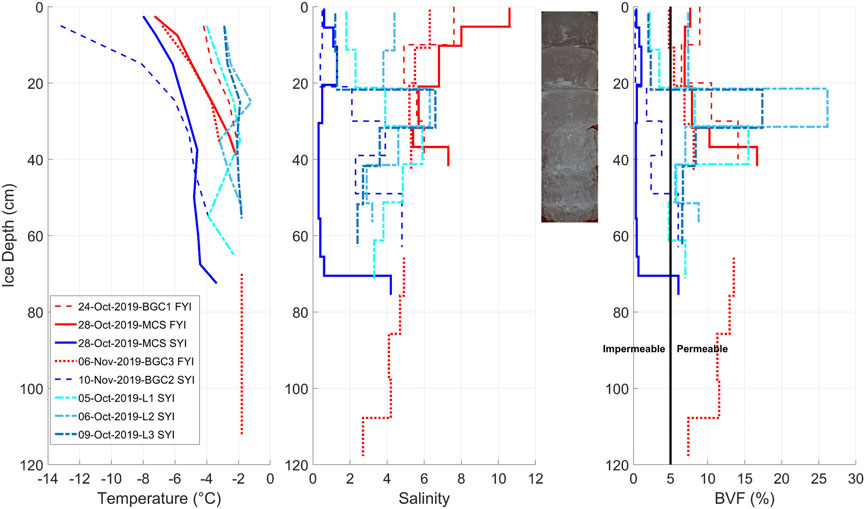
FIGURE 2. The initial (first site visit) temperature, salinity, and brine volume fraction (BVF) profiles taken from ice cores used for methane concentration analysis at the BGC sites, the main coring sites (MCS), and the Distributed Network. For the rafted FYI (BGC3), the ice mass below the seawater pocket was assumed to be isothermal because no temperature measurements were taken. The salinity profiles highlight the spatial variability of physical properties between FYI and SYI, as well as the variation within SYI. To show how the porous ice in the bottom segment of the ice in early autumn relate to the salinity profile, an ice core photograph from L2 is shown. The salinity for the 40–50 cm segment of L1 was linearly interpolated because of a leaking sample bag. The salinity and BVF profiles between each core are slightly offset vertically to ease visualization.

The SYI showed remarkable heterogeneity in its physical properties due to layers with very low salinity. These layers are usually the product of refrozen melt ponds or strongly desalinated residual ice layers during the previous summer melt. At the MCS-SYI site, the ice was rather fresh (salinity $<$ 1) down to a depth of 70 cm, hinting at strong desalination in this area. We observed a change in salinity from $<$ 1 to $>$ 4 at an ice depth of 70 cm, likely indicating the SYI to IFYI transition. The SYI at BGC2 consisted of freshwater ice in the upper 20 cm underlain by low salinity ice (2–4) from 20–50 cm, which we interpret as partially desalinated SYI. The salinity increased to $>$ 4 at an ice depth of 50 cm, representing the SYI to IFYI transition. At both MCS-SYI and BGC2, the entire ice slab above the SYI/IFYI boundary was impermeable. The initial physical properties at the DN SYI sites were quite different than at the CO, possibly because the first cores were taken in early October instead of late October. At the L sites, the salinity profiles generally showed low salinity ice (2–4) at the top of and bottom and a high salinity peak ($>$ 6) in the middle of the cores. The peak occurred at the visual horizon from solid ice to porous and brittle ice (Figure 2). Therefore, the peak may be the result of upwelling intrusive seawater that froze in the SYI voids.

The generally more saline conditions of the residual ice at the L sites point to the CO SYI sites having been more affected by melt ponds and more enhanced desalination of the SYI. The freshwater nature of these sites has considerable impacts on the sea ice growth and permeability evolution from autumn to spring. Therefore, the initial floe conditions described here serve as a benchmark for the time series description and discussion. For the description of the results, the time series are split into four phases as follows:

• Phase I: Early ice growth phase in autumn with warm air intrusions (late October to December)

• Phase II: Gradual freeze with no warm air intrusions (December to mid-January)

• Phase III: Coldest growth period and ice rafting (mid-January to mid-March)

• Phase IV: Initial spring warming (mid-March to early May)

These phases highlight when the FYI time series transitioned to rafted FYI at the MCS and changing upper boundary conditions that can affect the ice permeability and CRG pathways. The air temperature and snow thickness observed during ice coring are presented for each time series.

4.2 Phase I: Early Ice Growth Phase in Autumn With Warm Air Intrusions (late October to December)

4.2.1 First-Year Ice

At the start of the time series in late October, FYI exhibited typical C-shaped salinity profiles at BGC1 (Figure 3) and MCS-FYI (Figure 4). This pattern is in accordance with prior field studies and numerical modelling of FYI growth (Cox and Weeks, 1988). The C-shape revealed ongoing brine entrapment and gravity drainage as the main salt transport processes during this period. From late October to mid-November, the ice surface temperature decreased and the top of the ice eventually became impermeable. However, during this time, the bottom half of the ice column was always permeable and allowed brine drainage to continue. This shifted the original C-shaped profile to a less saline regime with less curvature. When considering the average value of all adjacent cores, the brine drainage induced a salinity decrease of approximately 16% in the upper 10 cm at BGC1 from 24 October to 14 November.

FIGURE 3

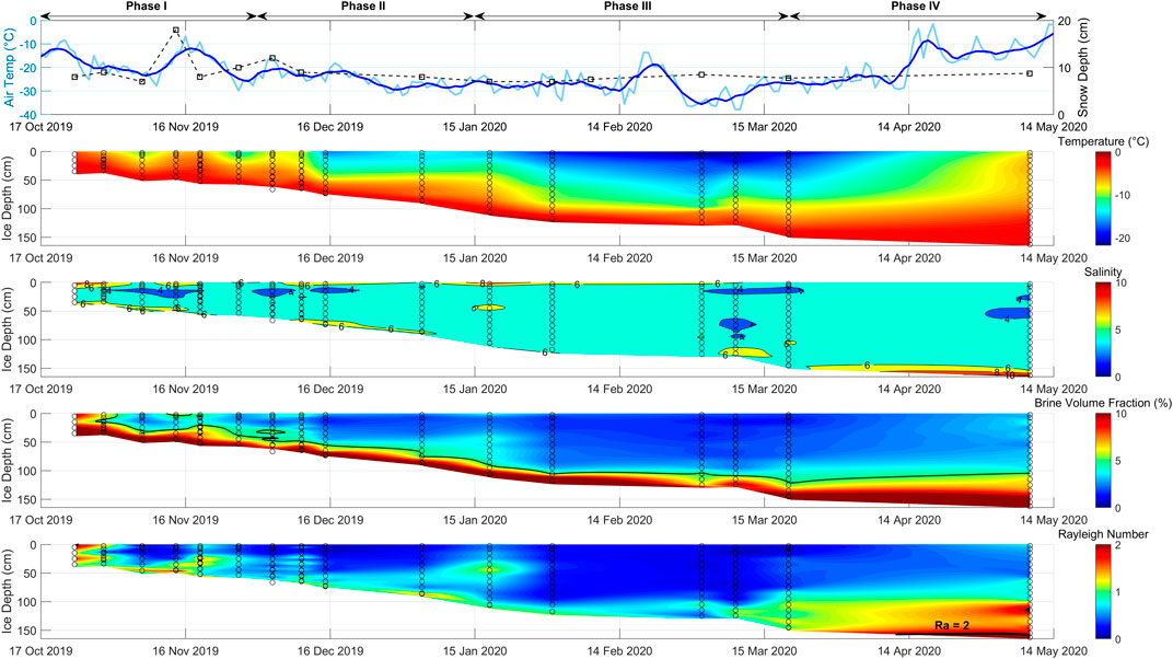
FIGURE 3. The evolution of temperature, salinity, brine volume fraction (BVF), and the Rayleigh number (Ra) at the BGC1 first-year ice site. The top panel shows the mean daily air temperature (light blue line) with a 7-day centered moving average (dark blue line) based on RV Polarstern onboard measurements and snow depth (dotted black line). The black circles represent ice sample midpoints, where values were stored to generate the interpolated fields. The thick black line in the BVF subplot indicates the 5% BVF contour and hence the assumed boundary between impermeable (BVF < 5%) and permeable (BVF ≥ 5%) ice. The BVF color bar is capped at 10%. The Ra color bar was capped at 2, which represents the minimum theoretical threshold for brine gravity drainage to occur based on the temperature and salinity. For the first coring date (24 October 2019), only the core with the maximum Ra number is shown.

FIGURE 4

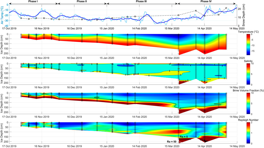
FIGURE 4. The evolution of physical properties at the main coring first-year ice site. See Figure 3 caption for a description of common labels and annotations. The FYI field rafted over a thinner and presumably younger and more saline ice floe and such ice cores were extracted on two occasions (21 March and 14 April). The ice thickness trend in spring is affected by both temporal and spatial variability.

In mid-November (15–20 November 2019), a storm with a warm air intrusion (WAI) exposed the ice surface to October-like temperatures, causing ice temperatures to warm up. Consequently, the sea ice column redeveloped permeable conditions at the top of the sea ice at BGC1 and throughout the entire ice column at the MCS. Since sea ice temperatures respond readily to atmospheric forcing, the onset of the WAI’s warming influence might have occurred before the 19 November coring date. Brine movement allowed the C-shape morphology to deviate from the expected shape for thin FYI, meaning that the peak salinity occasionally occurred at the bottom instead of the top of the sea ice by early December after the WAI. Interestingly, this phenomenon has been observed in the Bellingshausen Sea in the Antarctic (Carnat et al., 2016). We suggest that WAIs in late autumn may contribute to enhanced brine drainage in FYI by increasing the minimum BVF and thus the effective permeability in the ice column. After the WAI, low salinity layers of $<$ 4 for FYI were often observed temporally. The latter is less than the salinity of typical FYI. We suspect that the low salinity pockets developed in the middle of the ice column because this ice depth range provided the necessary brine density gradient and effective permeability to trigger brine release. This is not reflected in the Ra numbers, presumably because we are seeing the results of the WAI’s impact as opposed to a precursor for impending drainage.

At site BGC3, the FYI was up to 117 cm thick in early November (Figure 5), which numerical models indicate is unusually thick for FYI at this time of the year (Leppäranta, 1993). Since the initial salinity profile was $>4$ for the upper 100 cm, we interpreted BGC3 as rafted ice with two FYI slabs. In fact, a 20 cm thick seawater pocket was measured between 40 and 60 cm by inserting the ice thickness gauge down to the deeper ice slab after the shallower ice slab was extracted with the corer. At first, the ice temperatures were warm ($>$ −5°C) and the BVF exceeded 5% throughout the entire column, suggesting that it was permeable between the sea ice surface and ocean. By mid-November, the seawater pocket was no longer observed, presumably because it refroze or it was was not initially present in some areas. The decrease in maximum ice thickness from 117 to 104 cm supports the spatial variability argument, but given the heterogeneity and uncertainty associated with rafted ice, all the ice cores are shown in the time series. Under a relatively fresh surface layer with salinity $<$ 4, the salinity was mostly homogeneous with values between 4 and 6. Until the end of the initial growth phase, the 5% BVF contour remained at an ice depth of 50 cm, and therefore the bottom half of the ice was permeable. Despite the permeable nature of the ice, the Ra remained below 2, thereby suggesting no desalination. The latter is in accordance with the salinity time series.

FIGURE 5

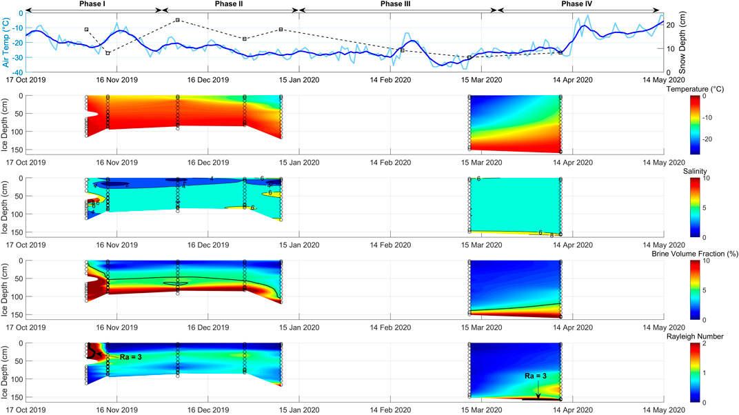
FIGURE 5. The evolution of physical properties at the BGC3 site. See Figure 3 caption for a description of common labels and annotations. In early November, a seawater pocket was encountered where the ice column consisted of two FYI layers affected by rafting.

4.2.2 Second-Year Ice

Compared to FYI, the residual ice which became SYI had a low salinity, especially in the strongly desalinated surface layer at the MCS, which resulted in lower permeability compared to saltier FYI. We describe the structure of SYI from top to bottom as refrozen melt ponds (if present) underlain by residual SYI. The freezing point of the frozen melt ponds was at, or slightly below, 0°C, rendering the permeability stable to cryotic ($<$ 0°C) temperature changes. On the other hand, the FYI developed permeable conditions when the ice surface temperature reached −5°C. The BVF of partially desalinated SYI is typically more sensitive to temperature than SYI with refrozen melt ponds, because it is characterized by a salinity in between freshwater ice and FYI. SYI has undergone significant brine drainage and flushing during its first summer melt season (Vancoppenolle et al., 2006), but can still have a salinity of around 2 as shown in prior studies (Granskog et al., 2017). At BGC2, the storm-induced warming resulted in a BVF between 2% and 3% in the SYI-layer beneath a fresh ice layer possibly from a refrozen melt pond (Figure 6), but the ice was still impermeable. During leg 1, additional sub-plots of BGC2 that were not part of the main time series were also cored. One of these sites contained actively refreezing freshwater pockets in November. At MCS-SYI, the low-salinity layer was about 70 cm thick, resulting in very low BVF in this layer throughout the time series (Figure 7). As a result, the impermeable to permeable transition always occurred at the interface between SYI and IFYI during the early ice growth phase. Overall, SYI acted as a low-permeability layer presumably hindering the sea ice-atmosphere interaction much earlier than near-surface FYI. The discrepancy between SYI with and without refrozen melt ponds was negligible in terms of permeability.

FIGURE 6

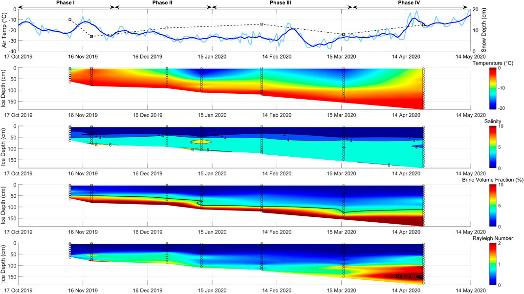
FIGURE 6. The evolution of physical properties at the BGC2 second-year ice site. See Figure 3 caption for a description of common labels and annotations.

FIGURE 7

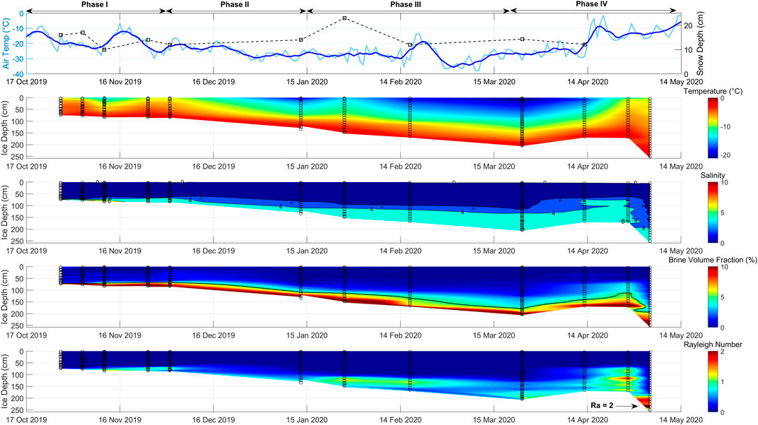
FIGURE 7. The evolution of physical properties at the main coring second-year ice site. See Figure 3 caption for a description of common labels and annotations. The relatively fresh SYI layer thickness above new ice growth varied spatially. The ice thickness trend is affected by both temporal and spatial variability.

4.2.3 Insulated First-Year Ice

Compared to FYI, IFYI showed a near-vertical or L-shaped salinity profile. The missing salinity increase near the surface typical for C-shaped profiles mainly results from the thermal buffering capacity of the SYI layer and the less turbulent conditions inhibiting frazil ice growth. The SYI insulated the IFYI from the atmosphere, resulting in a slower growth rate for IFYI in early winter, favoring less brine entrapment. Since the temperature gradient for thicker sea ice is weaker, the IFYI growth rate was initially slower compared to typical FYI. As a result of the slower ice growth rate and less turbulent conditions for ice formation, the salinity near the top of IFYI was lower than the salinity at the surface of FYI at the early stages of growth. Despite the lower salinity for IFYI compared to FYI, the IFYI was still permeable during the early growth phase because of its warmer temperature close to the seawater. The IFYI was permeable before and during the mid-November WAI. Even as ice temperatures decreased after the WAI, most of the IFYI was still permeable, because any cooling at the top of IFYI lagged behind cooling at the top of SYI. Overall, upper parts of IFYI was younger, less saline, and more insulated from transient ice surface temperature changes compared to surface FYI in the early growth phase. Consequently, the IFYI did not show the same distribution of low salinity pockets as FYI, resulting in a much more homogeneous ice salinity. The SYI shielded the IFYI from the mid-November WAI’s effects during the initial stage of IFYI formation.

4.3 Phase II: Gradual Freeze Without Warm Air Intrusions (December to Mid-January)

4.3.1 First-Year Ice

Since there were no obvious changes to the C-shaped salinity profiles, there was little salt expulsion in the ice column. Even though the surface ice temperatures showed a gradual negative trend, the thermal regime of the ice still changed in response to its increasing thickness. As the ice grew and cooled, the impermeable/permeable interface descended to 90 cm from the ice/snow interface at BGC1 and 80 cm at the MCS. While the permeable ice layer thickness remained constant, the permeable ice fraction in the ice column decreased as the gradual freezing progressed (Figures 3, 4).

4.3.2 Second-Year Ice

From December to mid-January, the impermeable/permeable boundary descended below the bottom of the SYI to 110 cm at the MCS and 90 cm at BGC2. Similar to the first phase, the BVF in the SYI layers was low because of the very low salinity. At BGC2, the BVF differences between refrozen melt ponds and typical SYI layers were insignificant and a more homogenous SYI layer developed. As during the early freezing period, the SYI-layers were an impermeable barrier (Figures 6, 7).

4.3.3 Insulated First-Year Ice

While the IFYI remained permeable in phase I, the top of the IFYI cooled and became impermeable in phase II (Figures 6, 7). Since the descent of the impermeable boundary below the SYI kept pace with IFYI formation, the thickness of permeable IFYI remained constant, while the fraction of permeable ice in the IFYI decreased at BGC2 (Figure 6). The salinity contours within the MCS IFYI sloped to greater ice depths versus time, hinting that there was a slow transport of salt towards the ice bottom (Figure 7). However, the Ra numbers ($<$ 1) were well below the minimum threshold for brine gravity drainage to occur. Since brine movement from brine expulsion is a very slow process (Notz, 2005), the spatial variability of the initial SYI thickness is the most plausible explanation for the dipping salinity contours at the MCS. Contrary to the MCS, the salinity contours in the IFYI at BGC2 remained at the same ice depth versus time.

4.4 Phase III: Coldest Growth Period and Ice Rafting Dynamics (Mid-January to Mid-March

4.4.1 First-Year Ice

From mid-January to March, the sea ice at the snow/ice interface cooled to its lowest annual temperature, reaching −20°C or lower at the surface. However, the ice thickness evolution at BGC1 (Figure 3) and MCS-FYI (Figure 4) were strikingly different. The sudden jump on 21 March in ice thickness at the MCS was due to ice rafting. The sea ice from the earlier phases of the time series rafted over a piece of thinner and presumably younger sea ice. For simplicity, the underlying ice slab is described as the “rafted ice mass.” At BGC1, no rafted ice was observed.

At the MCS, the rafted ice showed an increase in salinity at the ice bottom. From mid-February to mid-March, the ice thickness increased from 115 to 220 cm. Since BGC1 was not subject to ice rafting, its 150 cm thickness represents normal FYI growth conditions. This implies that the rafted ice mass at the MCS was only 70 cm thick and thus younger and therefore likely saltier than the main FYI mass on top. Since the rafted ice mass was younger, it started to form later in the freezing season during colder conditions. Since brine entrapment is more effective during rapid freezing, the rafted ice mass had a higher salinity. As a result, the salinity profile showed a very pronounced peak at the ice/water interface. For example, the salinity and BVF in the bottom 30 cm of the ice (190–220 cm) were 15 and 25%, respectively. The bottom 30 cm of the ice was soft and contained slush, due either to partially frozen seawater and/or perhaps a layer of platelet ice. Platelet ice was observed beneath the MOSAiC CO with a remotely operated underwater vehicle (ROV) (Katlein et al., 2020). However, the thin sections of the associated ice cores at the ROV sites revealed only weak evidence of platelet ice, likely because rapid congelation ice growth concealed the platelet ice signature (Katlein et al., 2020). Overall, the bottom 50 cm of the ice at the MCS was permeable and possibly just below the freezing point in the case of platelet ice. Furthermore, the bottom 30 cm of the ice at the MCS had a Ra number exceeding 50 and was thus very susceptible to impending brine gravity drainage.

Despite a decreasing growth rate at BGC1, there was no corresponding reduction in the salinity for newly formed ice. In mid-February, the ice floe drifted towards the Fram Strait and was increasingly affected by warmer and more saline Atlantic water (Rabe et al., 2022). The absolute salinity increased from approximately 32–34 g kg⁻¹ during the mid-February to April period, but likely had a minimal impact on the salinity of new ice. Differential ice growth rates, brine loss upon core extraction, as well as brine drainage between the freeze-up date and the date of core extraction, are other factors contributing to bottom ice salinity changes.

For FYI, a rafting event in winter has important implications for how the ice’s physical properties evolve during spring warming. Hence, FYI now branches into two categories: 1) level FYI, and 2) rafted FYI.

4.4.2 Second-Year Ice

Like phases I and II, the SYI remained an impermeable ice layer. However, the temperature of the SYI still decreased to the point where the upper 100 cm of the ice was below −10°C by mid-March. The freezing point of the fresh SYI is only slightly below 0°C rather than close to the freezing point of seawater (approximately −1.8°C). Since the fresh SYI layers do not contain brine, less energy is required to bring it to the melting point compared to FYI. However, at the melting point, more energy is required to melt fresh SYI compared to salty FYI.

4.4.3 Insulated First-Year Ice

The IFYI at the MCS appeared to experience an accelerated growth rate in mid-January, but this was only because the overlying SYI layer thickness showed considerable variability (Figure 7). At BGC2, the IFYI growth rate appeared constant and the overlying SYI thickness was more consistent during the drift (Figure 8). As during the previous phase, the IFYI temperature and salinity profiles varied less than FYI because of the insulating effect of the overlying SYI.

FIGURE 8

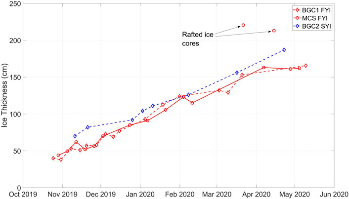
FIGURE 8. Maximum ice thickness observations for BGC1, the main coring (MCS) FYI site, and the BGC2 SYI sites are plotted as a function of time. Since the MCS SYI site had a highly variable SYI thickness overlying the insulated FYI, it is not presented. Site BGC3 is not included, because the initial thickness was affected by ice rafting.

4.5 Phase IV: Initial Spring Warming (Mid-March to Early May)

4.5.1 First-Year Ice

Consequences of Typical Ice Growth in Preceding Phase III

From mid-March to early May, the ice thickness at BGC1 increased from 150 to 165 cm. The slower growth rate was caused by the warmer air temperatures, but also transient thermal properties of the ice. As the ice temperature increases, the bulk thermal conductivity of the ice decreases because the brine volume fraction increases. Furthermore, the effective heat capacity increases in response to phase change in the ice, resulting in a lower thermal diffusivity. The ice warming and nearly negligible growth rate allowed the permeable layer of the ice slab and Ra numbers to increase. Since desalination did not occur here, the salinity profile was L-shaped and retained its high salinities near the ice/ocean interface (Figure 3). Hence, Ra numbers at the ice bottom in early May were higher at BGC1 than at the MCS. At BGC1, the high Ra numbers indicated that the system was approaching desalination. Note that the salinity at the bottom-most sample at BGC1 ($>$ 10) is a sampling artifact, because the sample thickness was only 5 cm.

Potential Consequences of an Ice Rafting Event in Preceding Phase III

At the MCS, the highly permeable bottom ice (190–220 cm) was primed for earlier brine drainage in spring, as inferred from the convection onset derived from the Ra number. Furthermore, ice temperatures increased from mid-March to mid-April (Figure 4). Brine in the 190–200 cm interval of the rafted ice mass possibly drained as revealed by the downwards sloping salinity contours between the two coring dates intersecting the rafted ice mass. Nevertheless, the BVF and Ra values at the ice bottom on 14 April still indicated permeable and drainage-susceptible conditions. The warm highly saline bottom layer observed on 21 March could have been mixed with seawater upon core extraction, resulting in higher salinity compared to in situ rafted ice conditions. Therefore, our interpretation of brine drainage in the rafted ice mass could also be due to spatially varying rafted ice mass salinity.

From mid-April to early May, the observed ice thickness decreased from 200 to 160 cm, because we transitioned from a FYI field with rafted ice to a FYI field without rafted ice. In early May, the ice surface temperatures warmed by several degrees. As the ice warmed, the BVF in the entire ice column increased. Consequently, the impermeable boundary rose in the ice column by about 40 cm and new ice formation ceased. Since the ice growth stopped, the salinity peak at the bottom of the ice disappeared after brine drained into the ocean. Consequently, the C-shaped salinity profile developed more linearity.

4.5.2 Second-Year Ice

Although the top of the SYI temperatures increased by at least 10°C at both sites from mid-March to early May, the freshness of SYI (or presence of fresh layers) conditioned its impermeable state (Figures 6, 7). Even in early May, the SYI was impermeable because it consisted of fresh ice layers. Although the FYI remained impermeable at the surface, its BVF increased in response to warmer temperatures. Since the SYI’s BVF did not change, its thermal properties were still the same as during the previous phases. Therefore, we infer that the SYI’s capacity to transport heat was unaffected by spring warming.

4.5.3 Insulated First-Year Ice

At the MCS, the total ice thickness (SYI + IFYI) increased from 206 to 260 cm during the mid-March to early May period, with thinner ice thicknesses on intermittent coring dates due to spatial variability. Because of the spatial variability, the impermeable boundary appeared to rise in the ice column during the time series. Interestingly, the impermeable boundary descended in early May, but this was likely due to thicker overlying SYI. At BGC2, the SYI layer thickness was constant, allowing for a better evaluation of IFYI growth patterns. Compared to typical FYI, the IFYI at BGC2 continued to grow until early May, because the fresh SYI cap acted as an efficient heat transport conduit. Consequently, ice growth and associated brine entrapment occurred for longer for the IFYI. In terms of brine release, the bottom 60 cm of the IFYI at the MCS were still permeable in early May. However, given the increasing Ra numbers, it was approaching a brine gravity drainage event. At BGC2, the increasing Ra numbers from 100–190 cm suggest this portion of the IFYI was also approaching a brine gravity drainage event.

5 Discussion

5.1 Effects of Ice Type on the Sea Ice Growth

Key factors affecting sea ice growth include air temperature, the temperature gradient in the ice column, ocean heat flux, the thermal properties of sea ice, and snow cover (Cox and Weeks, 1988). While the coring sites on the central floe generally experienced the same air temperature, the thickness and characteristics of SYI influenced how IFYI evolved in comparison to FYI. In late October, the FYI was already 40 cm thick, while the IFYI was in its initial growth stage (5–10 cm). Overall, the growth rate of FYI at our sites was linear from autumn to winter (approximately 0.7 cm/day). The influence of decreasing air temperatures in winter was offset by the sea ice’s increasing thickness and thickening snowpack (where applicable), which reduced the thermal gradient. When sea ice temperatures rose in spring, the temperature gradient decreased further, resulting in ice growth rates of less than 0.2 cm/day by early May (Figure 8). For the sites shown in Figure 8, the snow cover thicknesses were similar. For BGC1, MCS-FYI, and BGC2, the mean and standard deviations of the snow depths were 9.0 ± 2.8, 10.7 ± 3.8, and 11.1 ± 3.1 cm, respectively. Hence, the relative difference in growth rates between these sites can likely be attributed to other factors. Although the snow thickness did not show an increasing trend versus time at BGC1, Wagner et al. (2021) showed that the snow water equivalent increased at their CO site from late October to early February. Compaction of the snowpack over time would increase its thermal conductivity to offset its buffering capacity to slow ice growth. Site BGC3 was the most variable in terms of snow with a mean and standard deviation of 13.0 ± 5.9 cm and the MCS-SYI site had the thickest snow (14.4 ± 3.7 cm).

The thermal properties of FYI vary with temperature. In particular, the atmospheric warming episode in mid-April likely affected the FYI, because the mean daily air temperature increased to −2°C. Considering that the mid-November WAI helped develop permeable ice conduits from the ice surface to the ocean when the mean daily air temperature increased to only −5°C, it is reasonable to assume that ice near the ice/snow interface also became permeable in mid-April even though no ice cores were extracted in the mid-April WAI to verify this. Ice mass buoy data from the DN, however, show a clear warming signal in the ice in mid-April (Koo et al., 2021). Sea ice responds quickly to surface temperature changes, so a shift towards −2°C in the sea ice would result in BVF values between 10% and 20% in the near-surface ice for salinities between 4 and 8 (Cox and Weeks, 1983). Consequently, a higher BVF would lower the thermal conductivity of the ice. Furthermore, the upper 15 cm of FYI at the MCS was characterized by relatively less dense granular ice as revealed by density measurements, as well as ice texture analyses from thin sections (Nicolaus et al., 2022). The lower density of granular ice fosters an even lower thermal conductivity compared to columnar ice. Although heat capacity has a greater influence than the thermal conductivity on the transient thermal diffusivity of ice when phase change occurs, latent heat effects must be considered during both warming and cooling phases, i.e. before and after the WAI in mid-April. This is why we emphasize the role of the thermal conductivity of ice for ice growth here.

The melt ponds on the overlying SYI in summer (e.g. at BGC2) need time to refreeze, which can delay the onset of IFYI formation (Flocco et al., 2015). The latter is corroborated by our field observations. Considering that initial IFYI thickness at the MCS was only 5–10 cm in October, IFYI growth likely started in mid to late October. For most of the winter, the IFYI growth rate is slower than that of FYI. Consequently, the total ice thicknesses of both FYI or IFYI beneath the SYI sites reach comparable values by mid-March if the SYI thickness is 50 cm or less. However, in spring, the growth patterns start to diverge again. The IFYI continues to grow towards the end of April at a faster rate than the FYI (which either decelerates or completely stops), because the overlying SYI’s thermal properties are the same in spring as they are in the autumn and winter. Since the SYI’s salinity is so low, the BVF does not change in response to warming, resulting in a nearly constant thermal conductivity.

The net result of these processes is that the low-salinity SYI layer acts as an efficient heat transport conduit, contributing to later IFYI growth in spring compared to normal FYI. In fact, the warmer the ice temperature, the larger the difference in thermal properties between FYI and SYI (Schwerdtfecer, 1963). Hence the differences are mostly relevant for the spring season. For example, the thermal conductivity of sea ice with a density of 900 kg m⁻³ decreases by approximately 15% and 30% if its temperature increases from −8°C to −1°C for salinities of 4 and 8, respectively. Since the mid-April WAI was a short episode, seasonal FYI thermal conductivity changes is likely only one factor that can explain the later IFYI growth in spring compared to FYI. At the SYI sites, the snow is fresh, but at the FYI sites, the snow contains salts. Wetter snow with brine has a higher thermal conductivity than dry snow (Steffen and DeMaria, 1996), meaning that the snow at the SYI sites may be more effective at shielding the sea ice from spring warming and WAIs and preserving the temperature gradient between the snow/ice and ice/ocean interfaces. Consequently, the IFYI can grow later in spring compared to FYI. Merkouriadi et al. (2020) demonstrated that thicker snow cover reduces the impact of WAIs on slowing ice growth. Thus, we suggest that snow with a lower thermal conductivity could have a similar effect compared to snow of equal thickness and a higher thermal conductivity. Considering the paucity of ice cores in spring, we also acknowledge that the ice thickness differences between the FYI and SYI sites in spring may also be due to spatial variability.

5.2 Ice-type Related Effects on Sea Ice Brine

Sea ice brine volume fraction is affected by ice type, atmospheric warming episodes, and dynamic forcing (Figure 9). While atmospheric events directly alter the temperature of the ice, sea ice dynamics redistribute ice slabs in the atmosphere-ice-ocean column, which in turn, affects ice temperature profiles. If the rafting event creates a water pocket, then this creates a thermal buffer, as well as a potentially isolated sink for brine drainage from the upper layer. In all situations, an increase in BVF can trigger an ice desalination event, but the timing of such events are influenced by enhanced thermal and mechanical disturbances.

FIGURE 9

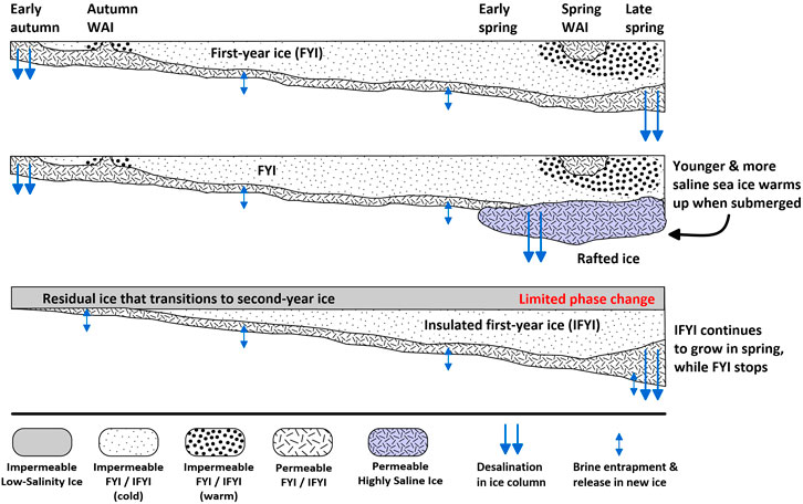
FIGURE 9. Some key processes affecting first-year ice (FYI), residual and second-year ice (SYI), and insulated first-year ice (IFYI) growth patterns, permeability, and desalination: atmospheric forcing, ice floe collisions, and ice-type dependent heat transport. The acronym WAI indicates “warm air intrusion.”

5.2.1 First-Year Ice

In late October when ice temperatures are relatively high, FYI is permeable over its whole depth. Consequently, desalination occurs in the ice column and lowers the ice salinity. During this time, atmosphere-ocean CRG exchange through the ice is theoretically possible. As the air temperature drops in early November, an impermeable layer develops at the surface of the FYI, presumably limiting CRG exchange with the atmosphere. However, since the sea ice is still in its early growth phase, the permeability boundary is very susceptible to short-term temperature fluctuations, especially at the surface, and this is why the mid-November WAI has a major impact on FYI permeability. The depth to the top of the deepest permeable layer readily responds to changes in the sea ice surface temperature from late October to early December. When the WAI reached the ice floe, FYI became permeable from the ice surface to the bottom. The re-development of permeable ice may foster further brine drainage from the sea ice, resulting in low salinity pockets.

From autumn to spring, the low salinity pockets were mainly concentrated in the upper 50 cm of the ice, because this was the average FYI thickness when the WAI reached the floe. The reason the low salinity pockets reveal themselves as isolated features in time and space is likely due to the spatial heterogeneity of the surface energy balance affected mainly by snow insulation, as well as the intrinsic properties of the ice and brine connectivity. Hypothetically, FYI fields with thicker snow cover would develop less permeable ice conditions during WAIs compared to areas with windswept surfaces and are thus less susceptible to warm spell-induced brine gravity drainage because the thicker snow effectively insulates the ice from air temperature changes.

After the WAI passes, the permeability evolution of FYI returns to a typical pattern, meaning that the impermeable boundary descends as the ice grows and cools in winter. The descent of the permeable boundary is most pronounced for level FYI at BGC3, because it had the thinnest snow cover (6 cm) during the coldest air temperature period of the drift in mid-March. For our sites, this phase lasts until mid-March when level FYI diverges into two paths: 1) level FYI, and 2) rafted FYI.

1. During spring warming, the impermeable boundary within level FYI rises in the ice column in response to warmer sea ice temperatures. Since the ice growth slows considerably, the slope between the depths to permeable ice versus permeable layer thickness is steep in comparison to SYI with a constant SYI-layer thickness. By early May, the Ra number suggests that a desalination event in FYI is approaching. The timing of such a desalination event fits with the numerical modelling of Vancoppenolle et al. (2006), who showed that the bottom 50 cm of FYI desalinates by brine gravity drainage in May during spring warming when the total ice thickness is approximately 150 cm thick. After this phase, the modelling shows that the top of the sea ice desalinates in late spring once ice surface melting and flushing occurs. During the melting phase, the Ra number vertical profile typically shows the highest values at the top of the sea ice when the entire ice column is permeable (e.g. Gourdal et al. (2019); Zhou et al. (2013)). Furthermore, the flushing phase occurs earlier for landfast sea ice compared to sea ice in the central Arctic Ocean. During the spring warming phase prior to melt, the highest Ra numbers occur in the bottom permeable region of the ice as indicated by our time series.

2. The situation of rafted ice is radically different, especially if the thinner FYI rafted under the main ice floe. Since the underlying ice is thinner than the original FYI field, it is presumably younger, meaning that it started to form later in the freezing season when air temperatures were colder and possibly during lead opening and closing. Colder conditions for ice growth foster more brine entrapment (Nakawo and Sinha, 1981), promoting more saline ice. Due to dynamic forcing, this rafted and more saline ice mass warms up following submergence, creating a thick and highly permeable FYI layer. Our results demonstrate that younger and more saline ice that rafts under FYI is primed for earlier desalination to the ocean. This priming may be influenced by how effectively the two ice slabs bond together by freezing, as well as the presence of water pockets. On the other hand, level FYI needs more time to develop the right conditions for convection, effectively delaying desalination to the ocean by approximately 1 month.

5.2.2 First-Year Ice With Seawater Pockets Generated by Rafting

In the previous paragraph, we discussed the impacts of dynamic forcing (i.e. rafting) on FYI permeability in late winter and early spring. But, what happens if rafting occurs very early in the ice growth phase like at BGC3? We suppose that seawater pockets created by rafting have interesting implications for brine gravity drainage. As shown in Figure 5, the ice layers above and below the water pocket are permeable, even in early November. The delayed onset of the impermeable surface layer is likely due to the relatively thick snow cover at this site (18 cm). Despite the entire ice slab being permeable, only the upper ice block can desalinate. This occurs, because the temperature of the seawater pocket is at approximately −1.8°C, effectively regulating the temperature of the deeper ice block and creating isothermal ice conditions. If the deeper ice block’s conditions are isothermal, then there is no brine density gradient within the ice to trigger drainage to the ocean. In fact, this ice may first become slushy and then dissolve. Of course, the former statement does not account for any brine drainage that might have occurred before the rafting event or before the lower ice block became isothermal. The upper ice block, however, can desalinate into the water pocket before the water pocket refreezes. This may be why a low salinity layer develops in the upper FYI block as the water pocket disappears. If the seawater pocket were isolated, then we would expect a highly saline ice layer to form as it refroze. Hence, the connectivity of the seawater pocket (open or closed state) to the underlying ocean likely determines if lateral exchanges play a role and the fate of the brine and its associated dissolved CRG contents that are released into it. In a closed system, one could imagine a highly concentrated saline layer that ultimately gets incorporated into the ice as the water pocket freezes and a potentially anoxic environment develops.

5.2.3 Second-Year Ice With Low-Salinity Ice Layers

The permeability evolution of the SYI sites is strikingly different compared to the FYI sites, because of the way SYI responds to temperature changes. In late autumn prior to the WAI, the impermeable boundary is flush with the SYI/IFYI interface and the IFYI is very thin due to the fresh ice layer’s influence at delaying basal ice growth. The relatively thick snow cover at MCS-SYI also contributes to delaying the growth of new ice. When the WAI encounters the floe, the sea ice temperatures increase. However, unlike FYI, the impermeable boundary remains at the same position, theoretically preventing any CRG exchange between the atmosphere and the ocean. The IFYI grows during this time, allowing the permeable ice layer to thicken. After the WAI passes and air temperatures decrease towards winter, the permeability evolution is quite similar to level FYI. In early December, the gap between the depths to the permeable layers at the FYI and SYI sites begins to close, because the sea ice enters a phase of prolonged cooling and its increasing thickness renders the permeable ice boundary less sensitive to ice surface temperature changes. This similarity lasts until mid-March, at which point the permeability evolution for IFYI starts to diverge from level FYI once again. Recall that during spring warming, the FYI stops growing and the IFYI continues to grow. Therefore, while the impermeable boundary rises in both FYI and IFYI, the permeable ice layer for the IFYI thickens. This results in a relatively weak slope between the depth to the permeable ice layer and permeable ice thickness for SYI sites with a consistent SYI-layer thickness like BGC2. Furthermore, the permeable ice thickness for IFYI is greater than for level FYI at the same time in spring. Similar to FYI, the increasing Ra numbers in the permeable ice layer suggests that a desalination event is approaching. We suspect that impending desalination events for the IFYI potentially release more brine than typical FYI, because the IFYI permeable ice thickness is greater. However, because of the low-salinity SYI layer, the impermeable boundary at SYI sites will ultimately ascend to the SYI/IFYI interface, while the impermeable boundary for typical FYI will rise to the ice surface. This means that the entire spring and summer desalination phase for IFYI will be shorter.

6 Implications for an Arctic With More Seasonal Ice

As suggested by satellite observations over the past three decades, warming has already led to an increase of 40% to 70% of the FYI areal fraction of sea ice cover in the Arctic in winter (Tschudi et al., 2020). Since FYI is more saline than old ice (SYI and MYI), our research supports the idea that this shift can have important consequences for sea ice physical properties and thus CRG exchange. For example, during the MOSAiC drift, we discovered that SYI was consistently an impermeable barrier from autumn to spring, presumably inhibiting CRG exchange between the atmosphere and ocean. This also applies to MYI, whose fraction of winter sea ice decreased by 28% from 1984 to 2018 (Stroeve and Notz, 2018). The SYI was characterized by low salinities, because they contained refrozen melt ponds or desalinated residual ice that had survived the last summer melt. Consequently, warm air intrusions (WAIs) in autumn increased the SYI temperature, but not its permeability. On the contrary, the FYI sites became permeable from the ice surface to the ice bottom in autumn during WAIs. As the Arctic warms, FYI may become less salty compared to “classical” FYI due to more permeable conditions in autumn. Accordingly, the drainage of brine containing dissolved CRG may occur earlier in the growth phase. From 1990 to 2012, there has been an increase in the frequency of WAIs originating from the North Atlantic and North Pacific during late autumn and early winter (Woods and Caballero, 2016). Further, there has been a noticeable increase in the number of extreme cyclones, especially in November and December (Rinke et al., 2017). The latter is consistent with increased number and duration warming events observed in the Atlantic sector of the Arctic during late autumn and winter (Graham et al., 2017). This warming delays the onset of FYI growth, thereby resulting in thinner late autumn FYI and facilitating permeable conduit development. If snow depth decreases concurrently (Webster et al., 2014; Stroeve et al., 2020), the ice’s thermal insulation will be reduced. The declining snow depth on Arctic sea ice serves to make the sea ice more sensitive to air temperature changes during these short-term events. In addition to an expanding FYI cover, the Arctic Ocean has also experienced an increase in the mean drift speed of sea ice from 1979 to 2007, possibly resulting in an increased deformation rate (Rampal et al., 2009). If rafting and ridging events become more pronounced, there may be increased submergence of lead ice. Our time series reveal that any form of presumably younger and more saline FYI submerged during ice rafting is pre-conditioned for earlier desalination to the ocean as well. The effects of WAIs in late autumn and a warmer and more dynamic FYI pack may result in enhanced autumn and earlier spring desalination events, respectively, shifting the magnitude and timing of downward directed CRG transport.

While the areal extent of SYI has only slightly increased since the 1980s, it is thinning, especially at the marginal ice zones (Mallett et al., 2021). Consequently, IFYI growth beneath SYI is enhanced (Petty et al., 2018), however, this is also largely dependent on snow depth on sea ice (Merkouriadi et al., 2017, 2020). More frequent WAIs in autumn can delay melt pond refreezing and the onset of IFYI growth, as inferred from numerical models of melt pond evolution (Flocco et al., 2015). However, our results suggest that the termination of IFYI growth in spring may occur later than FYI growth. While WAIs in spring similarly influence the temperature gradients of FYI and SYI fields (SYI + IFYI) with the same total ice thickness, their effects on the sea ice’s thermal properties depend strongly on salinity. As ice temperatures increase, the thermal conductivity of FYI decreases, while the thermal conductivity of nearly fresh SYI remains constant. In addition, the relatively dry and fresh snow at the SYI sites may better shield the sea ice from warming and contribute to later IFYI growth in spring. Given the observed increase in WAIs into the Arctic during spring (Kapsch et al., 2013), we expect reduced FYI growth in spring compared to IFYI.

7 Conclusion

We collected a time series of Arctic sea ice cores at multiple FYI and SYI sites representing a range of spatially variable ice conditions in the MOSAiC Central Observatory and within the surrounding Distributed Network from autumn to spring. For the first time, the evolution of sea ice permeability during the polar winter was tracked simultaneously for both ice types and with these new insights, we discussed how the development of different ice types could change in a warming Arctic with consequences for the preferred pathways of climate relevant gases (CRG) in sea ice. Some specific findings were:

• First-year ice was characterized by permeable conditions for brine containing dissolved CRG from the ice surface to the ocean in late October (early autumn)

• First-year ice re-developed permeable conditions for brine containing dissolved CRG from the ice surface to the ocean during warm air intrusions in mid-autumn

• Residual ice, that became second-year ice, was consistently an impermeable barrier from autumn to spring, presumably inhibiting CRG exchange between the atmosphere and ice

• Relatively young and more saline FYI submerged during ice rafting was pre-conditioned for earlier desalination to the ocean in spring compared to FYI that formed in autumn

• Later ice growth was observed beneath SYI compared to FYI in spring, prolonging the period of dissolved CRG uptake in sea ice

Overall, this study highlights downward directed CRG pathways to the ice/ocean interface in FYI and SYI by inferring sea ice permeability and potential brine release from several time series of temperature and salinity measurements from autumn to spring. Brine contains dissolved CRG; therefore, seasonal weather patterns and events like WAIs and ice rafting that influence permeability also determine the fate of CRG during the growth phase of sea ice. The physical properties presented in this paper lay the foundation for subsequent analyses on actual CRG contents measured in the ice cores, as well as air-ice and ice-ocean gas fluxes.

Data Availability Statement

The original contributions presented in the study are available in PANGAEA and the links are provided in the Supplementary Material. Further inquiries can be directed to the corresponding author.

Author Contributions

Contributed to conception and design: MA, ED, PSP, KA, DB, MAG, TK, MN, MO, AR, and CH. Contributed to acquisition of data: MA, ED, PSP, KA, DB, JB, GC, JC, AD, DVD, SF, NK, TK, CM, MO, AR, JS, TS, ES, MS, AU, JV, LW, and LZ. Contributed to analysis and interpretation of data: MA, ED, PSP, KA, DB, DVD, MAG, TK, MO, AR, JV, and CH. Drafted and/or revised the article: All authors. Approved submitted version for publication: All authors.

Funding

The work was funded by:

• German Federal Ministry for Education and Research (BMBF) through financing the Alfred-Wegener-Institut Helmholtz Zentrum für Polar-und Meeresforschung (AWI) and the RV Polarstern expedition PS122 under grant N-2014-H-060_Dethloff

• The AWI through its projects: AWI_ICE, AWI_SNOW, AWI_ECO, AWI_BGC

• German Research Foundation (DFG): 429838323

• German Research Foundation (DFG): 414169436

• German Research Foundation (DFG): TRR172-AC3 project (grant: 268020496)

• The Swedish Research Council Formas (grant: 2018-01398)

• Swedish Polar Research Secretariat

• The Research Council of Norway - through project HAVOC (grant: 280292)

• EU H2020 - ARICE (EU grant agreement: 730695)

• US National Science Foundation (NSF) Office of Polar Programs: OPP-1735862

• US National Science Foundation (NSF) Office of Polar Programs: OPP-1821911

• US National Science Foundation (NSF) Office of Polar Programs: OPP-1753423

• US National Science Foundation (NSF) Office of Polar Programs: OPP-1753418

• The National Aeronautics and Space Administration (NASA) Cryospheric Sciences Internal Scientist Funding Model (ISFM)

• Dutch Science Foundation (NWO) under the Polar Program, project number: 866.18.002

• Chinese Polar Environmental Comprehensive Investigation and Assessment Programs, funded by the Chinese Arctic and Antarctic Administration; National Natural Science Foundation of China (grant: 41676186)

Conflict of Interest

The reviewer BC declared a past co-authorship with the author MA to the handling editor.

The remaining authors declare that the research was conducted in the absence of any commercial or financial relationships that could be construed as a potential conflict of interest.

Publisher’s Note

All claims expressed in this article are solely those of the authors and do not necessarily represent those of their affiliated organizations, or those of the publisher, the editors and the reviewers. Any product that may be evaluated in this article, or claim that may be made by its manufacturer, is not guaranteed or endorsed by the publisher.

Acknowledgments

This work was carried out and data used in this manuscript was produced as part of the international Multidisciplinary drifting Observatory for the Study of the Arctic Climate (MOSAiC) with the tag MOSAiC20192020. We thank all persons involved in the expedition of the Research Vessel RV Polarstern during MOSAiC in 2019–2020 (AWI_PS122_00) as listed in Nixdorf et al. (2021). We highly acknowledge all the participants for the fieldwork at the main coring site, especially Allison Fong and Rob Rember during leg 1, Sinhue Torres Valdes during leg 2, and Clara Hoppe and Susanne Spahic during leg 3, who all contributed enormously to the development of a safe and efficient coring procedure. We also thank Markus Rex and Verena Mohaupt for their leadership on leg 1 of the MOSAiC drift campaign. Antonia Immerz also deserves credit for her tireless effort to assist us and all other teams with data management for the MOSAiC central storage and PANGAEA. As part of the Akademik Fedorov cruise, the ice coring program received support from Jari Haapala. We acknowledge the assistance of the students of the MOSAiC school led by Josefine Lenz. As part of the writing process, we thank Sandro Dahlke for helpful discussions about atmosphere-ice interactions.

References

Abrahamsson, K., Granfors, A., Ahnoff, M., Cuevas, C. A., and Saiz-Lopez, A. (2018). Organic Bromine Compounds Produced in Sea Ice in Antarctic Winter. Nat. Commun. 9, 1–8. doi:10.1038/s41467-018-07062-8

PubMed Abstract | CrossRef Full Text | Google Scholar

Angelopoulos, M., Damm, E., Simões Pereira, P., Abrahamsson, K., Bauch, D., Bowman, J. S., et al. (2022). Physical Properties of Sea Ice Cores for Biogeochemistry Studies Measured on Legs 1 to 3 of the MOSAiC Expedition. PANGAEA. doi:10.1594/PANGAEA.943811

CrossRef Full Text | Google Scholar

Assur, A. (1960). Composition of Sea Ice and its Tensile Strength, Vol. 44. Wilmette, Illinois: US Army Snow, Ice and Permafrost Research Establishment.

Google Scholar

Carnat, G., Brabant, F., Dumont, I., Vancoppenolle, M., Ackley, S. F., Fritsen, C., et al. (2016). Influence of Short-Term Synoptic Events and Snow Depth on DMS, DMSP, and DMSO Dynamics in Antarctic Spring Sea Ice. Elem. Sci. Anthropocene 4. doi:10.12952/journal.elementa.000135

CrossRef Full Text | Google Scholar

Comiso, J. C., Parkinson, C. L., Gersten, R., and Stock, L. (2008). Accelerated Decline in the Arctic Sea Ice Cover. Geophys. Res. Lett. 35. doi:10.1029/2007GL031972

CrossRef Full Text | Google Scholar

Cox, G. F. N., and Weeks, W. F. (1983). Equations for Determining the Gas and Brine Volumes in Sea-Ice Samples. J. Glaciol. 29, 306–316. doi:10.1017/s0022143000008364

CrossRef Full Text | Google Scholar

Cox, G. F. N., and Weeks, W. F. (1988). Numerical Simulations of the Profile Properties of Undeformed First-Year Sea Ice During the Growth Season. J. Geophys. Res. 93, 12449–12460. doi:10.1029/JC093iC10p12449

CrossRef Full Text | Google Scholar

Crabeck, O., Galley, R. J., Mercury, L., Delille, B., Tison, J. L., and Rysgaard, S. (2019). Evidence of Freezing Pressure in Sea Ice Discrete Brine Inclusions and its Impact on Aqueous‐Gaseous Equilibrium. J. Geophys. Res. Oceans 124, 1660–1678. doi:10.1029/2018JC014597

CrossRef Full Text | Google Scholar

Damm, E., Bauch, D., Krumpen, T., Rabe, B., Korhonen, M., Vinogradova, E., et al. (2018). The Transpolar Drift Conveys Methane from the Siberian Shelf to the Central Arctic Ocean. Sci. Rep. 8, 1–10. doi:10.1038/s41598-018-22801-z

PubMed Abstract | CrossRef Full Text | Google Scholar

Damm, E., Rudels, B., Schauer, U., Mau, S., and Dieckmann, G. (2015). Methane Excess in Arctic Surface Water- Triggered by Sea Ice Formation and Melting. Sci. Rep. 5, 1–9. doi:10.1038/srep16179

CrossRef Full Text | Google Scholar

Eicken, H. (1998). Deriving Modes and Rates of Ice Growth in the Weddell Sea from Microstructural, Salinity, and Stable-Isotope Data. Antarct. Res. Ser. 74, 89–122.

Google Scholar

Flocco, D., Feltham, D. L., Bailey, E., and Schroeder, D. (2015). The Refreezing of Melt Ponds on Arctic Sea Ice. J. Geophys. Res. Oceans 120, 647–659. doi:10.1002/2014JC010140

CrossRef Full Text | Google Scholar

Freitag, J. (1999). The Hydraulic Properties of Arctic Sea Ice-Implications for the Small-Scale Particle Transport. Rep. Polar Res. 325, 1–150. doi:10.2312/BzP_0325_1999

CrossRef Full Text | Google Scholar

Fukusako, S. (1990). Thermophysical Properties of Ice, Snow, and Sea Ice. Int. J. Thermophys. 11, 353–372. doi:10.1007/BF01133567

CrossRef Full Text | Google Scholar

Golden, K. M., Eicken, H., Heaton, A. L., Miner, J., Pringle, D. J., and Zhu, J. (2007). Thermal Evolution of Permeability and Microstructure in Sea Ice. Geophys. Res. Lett. 34. doi:10.1029/2007GL030447

CrossRef Full Text | Google Scholar

Gourdal, M., Crabeck, O., Lizotte, M., Galindo, V., Gosselin, M., Babin, M., et al. (2019). Upward Transport of Bottom-Ice Dimethyl Sulfide During Advanced Melting of Arctic First-Year Sea Ice. Elem. Sci. Anthropocene 7. doi:10.1525/elementa.370

CrossRef Full Text | Google Scholar

Graham, R. M., Cohen, L., Petty, A. A., Boisvert, L. N., Rinke, A., Hudson, S. R., et al. (2017). Increasing Frequency and Duration of Arctic Winter Warming Events. Geophys. Res. Lett. 44, 6974–6983. doi:10.1002/2017GL073395

CrossRef Full Text | Google Scholar

Granfors, A., Karlsson, A., Mattsson, E., Smith, W. O., and Abrahamsson, K. (2013). Contribution of Sea Ice in the Southern Ocean to the Cycling of Volatile Halogenated Organic Compounds. Geophys. Res. Lett. 40, 3950–3955. doi:10.1002/grl.50777

CrossRef Full Text | Google Scholar

Granskog, M. A., Rösel, A., Dodd, P. A., Divine, D., Gerland, S., Martma, T., et al. (2017). Snow Contribution to First-Year and Second-Year Arctic Sea Ice Mass Balance North of Svalbard. J. Geophys. Res. Oceans 122, 2539–2549. doi:10.1002/2016JC012398

CrossRef Full Text | Google Scholar

Hambler, C., and Henderson, P. A. (2022). Temperature, Carbon Dioxide and Methane. Res. Square. doi:10.21203/rs.3.rs-558940/v2

CrossRef Full Text | Google Scholar

Johnston, M. E. (2017). Seasonal Changes in the Properties of First-Year, Second-Year and Multi-Year Ice. Cold Regions Sci. Technol. 141, 36–53. doi:10.1016/j.coldregions.2017.05.006

CrossRef Full Text | Google Scholar

Kapsch, M.-L., Graversen, R. G., and Tjernström, M. (2013). Springtime Atmospheric Energy Transport and the Control of Arctic Summer Sea-Ice Extent. Nat. Clim. Change 3, 744–748. doi:10.1038/nclimate1884

CrossRef Full Text | Google Scholar

Katlein, C., Mohrholz, V., Sheikin, I., Itkin, P., Divine, D. V., Stroeve, J., et al. (2020). Platelet Ice Under Arctic Pack Ice in Winter. Geophys. Res. Lett. 47, e2020GL088898. doi:10.1029/2020GL088898

CrossRef Full Text | Google Scholar

Koo, Y., Lei, R., Cheng, Y., Cheng, B., Xie, H., Hoppmann, M., et al. (2021). Estimation of Thermodynamic and Dynamic Contributions to Sea Ice Growth in the Central Arctic Using ICESat-2 and MOSAiC SIMBA Buoy Data. Remote Sens. Environ. 267, 112730. doi:10.1016/j.rse.2021.112730

CrossRef Full Text | Google Scholar

Krumpen, T., Birrien, F., Kauker, F., Rackow, T., von Albedyll, L., Angelopoulos, M., et al. (2020). The MOSAiC Ice Floe: Sediment-Laden Survivor from the Siberian Shelf. Cryosphere 14, 2173–2187. doi:10.5194/tc-14-2173-2020,2020

CrossRef Full Text | Google Scholar

Krumpen, T., and Sokolov, V. (2020). The Expedition AF122/1: Setting up the MOSAiC Distributed Network in October 2019 with Research Vessel AKADEMIK FEDOROV. Rep. Polar Mar. Res. 744.

Google Scholar

Lange, B. A., Michel, C., Beckers, J. F., Casey, J. A., Flores, H., Hatam, I., et al. (2015). Comparing Springtime Ice-Algal Chlorophyll a and Physical Properties of Multi-Year and First-Year Sea Ice from the Lincoln Sea. PloS One 10, e0122418. doi:10.1371/journal.pone.0122418

PubMed Abstract | CrossRef Full Text | Google Scholar

Leppäranta, M. (1993). A Review of Analytical Models of Sea‐Ice Growth. Atmosphere-Ocean 31, 123–138. doi:10.1080/07055900.1993.9649465

CrossRef Full Text | Google Scholar

Leppäranta, M., and Manninen, T. (1988). “The Brine and Gas Content of Sea Ice with Attention to Low Salinities and High Temperatures,” in Tech. Rep. (Helsinki, Finland: Finnish Institute of Marine Research).

Google Scholar

Mallett, R. D. C., Stroeve, J. C., Tsamados, M., Landy, J. C., Willatt, R., Nandan, V., et al. (2021). Faster Decline and Higher Variability in the Sea Ice Thickness of the Marginal Arctic Seas When Accounting for Dynamic Snow Cover. Cryosphere 15, 2429–2450. doi:10.5194/tc-15-2429-2021

CrossRef Full Text | Google Scholar

Merkouriadi, I., Cheng, B., Graham, R. M., Rösel, A., and Granskog, M. A. (2017). Critical Role of Snow on Sea Ice Growth in the Atlantic Sector of the Arctic Ocean. Geophys. Res. Lett. 44, 479. doi:10.1002/2017GL075494

CrossRef Full Text | Google Scholar

Merkouriadi, I., Cheng, B., Hudson, S. R., and Granskog, M. A. (2020). Effect of Frequent Winter Warming Events (Storms) and Snow on Sea-Ice Growth - A Case from the Atlantic Sector of the Arctic Ocean During the N-Ice2015 Campaign. Ann. Glaciol. 61, 164–170. doi:10.1017/aog.2020.25

CrossRef Full Text | Google Scholar

Middleton, C. A., Thomas, C., De Wit, A., and Tison, J.-L. (2016). Visualizing Brine Channel Development and Convective Processes During Artificial Sea-Ice Growth Using Schlieren Optical Methods. J. Glaciol. 62, 1–17. doi:10.1017/jog.2015.1

CrossRef Full Text | Google Scholar

Nakawo, M., and Sinha, N. K. (1981). Growth Rate and Salinity Profile of First-Year Sea Ice in the High Arctic. J. Glaciol. 27, 315–330. doi:10.3189/S0022143000015409

CrossRef Full Text | Google Scholar

Nicolaus, M., Perovich, D., Spreen, G., Granskog, M., Albedyll, L., Angelopoulos, M., et al. (2022). Overview of the MOSAiC Expedition – Snow and Sea Ice. Elem. Sci. Anth 10, 000046. doi:10.1525/elementa.2021.000046

CrossRef Full Text | Google Scholar

Nixdorf, U., Dethloff, K., Rex, M., Shupe, M., Sommerfeld, A., Perovich, D. K., et al. (2021). MOSAiC Extended Acknowledgement. doi:10.5281/zenodo.5179739

CrossRef Full Text | Google Scholar

Notz, D. (2005). Thermodynamic and Fluid-Dynamical Processes in Sea Ice. Ph.D. thesis (Cambridge: University of Cambridge).

Notz, D., and Worster, M. G. (2009). Desalination Processes of Sea Ice Revisited. J. Geophys. Res. 114. doi:10.1029/2008JC004885

CrossRef Full Text | Google Scholar

Notz, D., and Worster, M. G. (2008). In Situ Measurements of the Evolution of Young Sea Ice. J. Geophys. Res. 113. doi:10.1029/2007JC004333

CrossRef Full Text | Google Scholar

Oggier, M., Eicken, H., Jin, M., and Høyland, K. (2020). Seasonal and Interannual Variability of Sea-Ice State Variables: Observations and Predictions for Landfast Ice in Northern Alaska and Svalbard. Cryosphere Discuss. 2020, 1–28. doi:10.5194/tc-2020-52

CrossRef Full Text | Google Scholar

Petty, A. A., Holland, M. M., Bailey, D. A., and Kurtz, N. T. (2018). Warm Arctic, Increased Winter Sea Ice Growth? Geophys. Res. Lett. 45, 12–922. doi:10.1029/2018GL079223

CrossRef Full Text | Google Scholar

Rabe, B., Heuzé, C., Regnery, J., Aksenov, Y., Allerholt, J., Athanase, M., et al. (2022). Overview of the Mosaic Expedition: Physical Oceanography. Elem. Sci. Anth 10, 00062. doi:10.1525/elementa.2021.00062

CrossRef Full Text | Google Scholar

Rampal, P., Weiss, J., and Marsan, D. (2009). Positive Trend in the Mean Speed and Deformation Rate of Arctic Sea Ice, 1979-2007. J. Geophys. Res. 114. doi:10.1029/2008JC005066

CrossRef Full Text | Google Scholar

Rinke, A., Maturilli, M., Graham, R. M., Matthes, H., Handorf, D., Cohen, L., et al. (2017). Extreme Cyclone Events in the Arctic: Wintertime Variability and Trends. Environ. Res. Lett. 12, 094006. doi:10.1088/1748-9326/aa7def

CrossRef Full Text | Google Scholar

Schmithüsen, H. (2021a). Continuous Meteorological Surface Measurement During POLARSTERN Cruise PS122/1. PANGAEA. Bremerhaven: Alfred Wegener Institute, Helmholtz Centre for Polar and Marine Research. doi:10.1594/PANGAEA.935221

CrossRef Full Text | Google Scholar

Schmithüsen, H. (2021b). Continuous Meteorological Surface Measurement During POLARSTERN Cruise PS122/2. PANGAEA. Bremerhaven: Alfred Wegener Institute, Helmholtz Centre for Polar and Marine Research. doi:10.1594/PANGAEA.935222

CrossRef Full Text | Google Scholar

Schmithüsen, H. (2021c). Continuous Meteorological Surface Measurement During POLARSTERN Cruise PS122/3. PANGAEA. Bremerhaven: Alfred Wegener Institute, Helmholtz Centre for Polar and Marine Research. doi:10.1594/PANGAEA.935223

CrossRef Full Text | Google Scholar

Schwerdtfecer, P. (1963). The Thermal Properties of Sea Ice. J. Glaciol. 4, 789–807. doi:10.3189/S0022143000028379

CrossRef Full Text | Google Scholar

Shupe, M. D., Rex, M., Blomquist, B., Persson, P. O. G., Schmale, J., Uttal, T., et al. (2022). Overview of the Mosaic Expedition: Atmosphere. Elem. Sci. Anth. 10, 00060. doi:10.1525/elementa.2021.00060

CrossRef Full Text | Google Scholar

Steffen, K., and DeMaria, T. (1996). Surface Energy Fluxes of Arctic Winter Sea Ice in Barrow Strait. J. Appl. Meteor. 35, 2067–2079. doi:10.1175/1520-0450(1996)035<2067:sefoaw>2.0.co;2

CrossRef Full Text | Google Scholar

Stroeve, J., Liston, G. E., Buzzard, S., Zhou, L., Mallett, R., Barrett, A., et al. (2020). A Lagrangian Snow Evolution System for Sea Ice Applications (SnowModel‐LG): Part II-Analyses. J. Geophys. Res. Oceans 125, e2019JC015900. doi:10.1029/2019JC015900

CrossRef Full Text | Google Scholar

Stroeve, J., and Notz, D. (2018). Changing State of Arctic Sea Ice Across All Seasons. Environ. Res. Lett. 13, 103001. doi:10.1088/1748-9326/aade56

CrossRef Full Text | Google Scholar

Tison, J. L., Delille, B., and Papadimitriou, S. (2017). “Gases in Sea Ice,” in Gases in Sea Ice (Chichester, UK: John Wiley & Sons), 433–471. Chap. 18. doi:10.1002/9781118778371.ch18

CrossRef Full Text | Google Scholar

Tschudi, M. A., Meier, W. N., and Stewart, J. S. (2020). An Enhancement to Sea Ice Motion and Age Products at the National Snow and Ice Data Center (NSIDC). Cryosphere 14, 1519–1536. doi:10.5194/tc-14-1519-2020

CrossRef Full Text | Google Scholar

Van der Linden, F. C., Tison, J. L., Champenois, W., Moreau, S., Carnat, G., Kotovitch, M., et al. (2020). Sea Ice CO₂ Dynamics across Seasons: Impact of Processes at the Interfaces. J. Geophys. Res. Oceans 125, e2019JC015807. doi:10.1029/2019JC015807

CrossRef Full Text | Google Scholar

Vancoppenolle, M., Fichefet, T., and Bitz, C. M. (2006). Modeling the Salinity Profile of Undeformed Arctic Sea Ice. Geophys. Res. Lett. 33. doi:10.1029/2006GL028342

CrossRef Full Text | Google Scholar

Vancoppenolle, M., Fichefet, T., and Bitz, C. M. (2005). On the Sensitivity of Undeformed Arctic Sea Ice to its Vertical Salinity Profile. Geophys. Res. Lett. 32. doi:10.1029/2005GL023427

CrossRef Full Text | Google Scholar

Verdugo, J., Damm, E., and Nikolopoulos, A. (2020). Methane Cycling within Sea Ice: Results from Drifting Ice During Late Spring, North of Svalbard. Cryosphere 15, 2701–2717. doi:10.5194/tc-15-2701-2021

CrossRef Full Text | Google Scholar

Wagner, D. N., Shupe, M. D., Persson, O. G., Uttal, T., Frey, M. M., Kirchgaessner, A., et al. (2021). Snowfall and Snow Accumulation Processes During the MOSAiC Winter and Spring Season. Cryosphere Discuss. 2021, 1–48. doi:10.5194/tc-2021-126

CrossRef Full Text | Google Scholar

Webster, M. A., Rigor, I. G., Nghiem, S. V., Kurtz, N. T., Farrell, S. L., Perovich, D. K., et al. (2014). Interdecadal Changes in Snow Depth on Arctic Sea Ice. J. Geophys. Res. Oceans 119, 5395–5406. doi:10.1002/2014JC009985

CrossRef Full Text | Google Scholar

WMO (2014). “World Meteorological Organization (WMO) Sea Ice Nomenclature: WMO-No. 259 Supplement to Vol. I, II and II, 5th Session of JCOMM Expert Team on Sea Ice,” in Tech. Rep. (Geneva: World Meteorological Organization).

Google Scholar

Woods, C., and Caballero, R. (2016). The Role of Moist Intrusions in Winter Arctic Warming and Sea Ice Decline. J. Clim. 29, 4473–4485. doi:10.1175/JCLI-D-15-0773.1

CrossRef Full Text | Google Scholar

Zhou, J., Delille, B., Eicken, H., Vancoppenolle, M., Brabant, F., Carnat, G., et al. (2013). Physical and Biogeochemical Properties in Landfast Sea Ice (Barrow, Alaska): Insights on Brine and Gas Dynamics Across Seasons. J. Geophys. Res. Oceans 118, 3172–3189. doi:10.1002/jgrc.20232

CrossRef Full Text | Google Scholar