 Franz A. Livio1*
 Francesco Bovo2
 Fabio Gabrieli2Roberto Gambillara1
 Sandro Rossato3
 Silvana Martin3
 Alessandro M. Michetti1,4
- 1Università Degli Studi Dell’Insubria, Dipartimento di Scienza ed Alta Tecnologia, Como, Italy
- 2Università di Padova, Dipartimento di Ingegneria Civile Edile e Ambientale (DICEA), Padova, Italy
- 3Università di Padova, Dipartimento di Geoscienze, Padova, Italy
- 4INGV Istituto Nazionale di Geofisica e Vulcanologia, Napoli, Italy
We investigated the Mt. Peron niche area of the Masiere di Vedana rock avalanche (BL), one of the major mass movements that affected the Eastern Southern Alps in historical times. So far, a geomechanical characterization and a stability analysis of the niche area, where potential rockfall sources are present, are lacking. The Mt. Peron niche area is a rocky cliff almost inaccessible to field-based measurements. In order to overcome this issue, we performed a geo-structural characterization of a sector of the cliff by means of a UAV-based photogrammetric survey. From the virtual outcrop, we extracted the orientation of 159 fractures that were divided into sets based on a K-means clustering algorithm and field-checked with some measurements collected along a rappelling descent route down to the cliff. Finally, with the aim of evaluating the stability of the volume under investigation, we performed a stability analysis of three rock pillars included in our survey by means of a distinct element numerical simulation. Our results indicate that two out of the three pillars are characterized by a stable state, under the simulation assumptions, whereas the third is close to failure, and for this reason, its condition needs further investigation.
Introduction
In the last ca. 30 years, analysis and monitoring of landslides have benefitted from remote sensing (Delacourt et al., 2007; Scaioni et al., 2014), including optical remote sensing (Mondini et al., 2011), SAR interferometry (e.g., Schlögel et al., 2015) and time series analysis (e.g., Liu et al., 2013), LiDAR (Ventura et al., 2011; Jaboyedoff et al., 2012), and optical correlation (Leprince et al., 2008; Travelletti et al., 2012).
Amongst the sectors of the landslides, the uppermost one is the toughest to investigate, due to the common presence of steep slopes, limited accessibility, and poor visibility from a near zenithal perspective (i.e., the satellite and aerial one). On the other hand, this area hosts some of the most important features in the characterization of landslides: the crown, the lateral flanks, the higher detachment scarps, and, possibly, the uppermost part of the deposit. In this article, for the sake of conciseness, we will refer to this complex area as “niche”. Niche areas can benefit from terrestrial-based remote sensing or, more recently, from imagery taken from an oblique aerial perspective, following the introduction of camera-equipped unmanned aerial vehicles (UAVs; see Nex and Remondino, 2014). The latter solution offers high flexibility of the scale range, avoids the possible logistic problems connected with ground-based instruments, and allows the choice of optimal perspectives in comparison to aerial-borne surveys. Moreover, a collection of digital images of the terrain, taken from different perspectives, can be used to reconstruct a 3D model of the ground surface (i.e., a virtual outcrop) and consequently to collect structural measurements and monitor areas not reachable by other means (Ruggles et al., 2016; Cawood et al., 2017; Esposito et al., 2017).
The reconstruction of 3D point clouds by means of close-range photogrammetry (i.e., a workflow of digital image processing, including Structure from Motion and Multi-View Stereo (SfM-MvS) (Gallup et al., 2007; Goesele et al., 2007; Jancosek et al., 2009; Westoby et al., 2012), has gained an increasing interest in the scientific community since the middle 90s. This approach was more recently boosted by the spreading of high-resolution digital cameras, increasing capabilities of personal computers, and the development of cloud computing. With the matching of a set of photographs, representing the same object from slightly different points of view, camera positions are calculated (SfM) and a 3D point cloud is reconstructed (MvS) representing the Digital Surface Model of the ground (DSM). The output is similar to the DSM reconstructed through a LiDAR survey even though the SfM-MvS does not offer the penetrative potential of laser pulses. Nevertheless, in poorly vegetated areas, it is an effective and low-cost alternative to airborne or terrestrial LiDAR (e.g., Fonstad et al., 2013; Cawood et al., 2017; Cook, 2017). UAVs equipped with high-resolution cameras considerably expanded the acquisition potential of data by means of this technique.
In this article, we present the results of a study performed on the Mt. Peron (1,486 m a.s.l.) niche area of the Masiere di Vedana rock avalanche (e.g., Pellegrini et al., 2006; Rossato et al., 2020), one of the major mass movements that occurred in the Eastern Southern Alps in historical times (Rossato et al., 2018). The mechanisms and dynamics of this landslide are still debated (see Rossato et al., 2020 for a review) whereas the deposits have been well studied (Genevois et al., 2006; Pellegrini et al., 2006; Rossato et al., 2020). Less effort has been spent so far on the characterization of the niche area, a sub-vertical rock cliff, ca. 800 m wide and 500 m high, that poses a significant landslide hazard due to impending blocks prone to rockfalls. Geomechanical analysis of the niche area would require detailed structural measurements that are largely lacking due to the objective difficulty to reach many sectors of the near-vertical rock cliffs.
We performed a UAV-based photographic survey of a sector of the niche area and built a virtual outcrop of the rock walls and measured a large number of fractures. Digital discontinuity orientations were compared with measurements taken at the base of the rock cliff, in the summit area, and along a rappel descent. The data obtained in the virtual outcrop were then used to run numerical simulations for the stability analysis of three pillars of the cliff, by means of a distinct element model with the ultimate goal of evaluating which pillars are in the less stable condition and therefore highlighting the need to concentrate further surveys and future analyzes (e.g., of brittle failure and runout) on these latest areas.
The Mt. Peron Niche Area: Geological and Geomorphological Setting
From a geological point of view (Figure 1), the Mt. Peron niche is located between two important regional structures: to the north, the Val Carpenada-Val Vido-Val Madonuta thrust (CVM) and, to the south, the Belluno thrust (BL) and the Belluno syncline (BS). The dominant lithologies are Triassic limestones and dolomites belonging to the Trento platform and close to the boundary with the Belluno through. In the upper sector of the Cordevole river, the metamorphic basement and Permian sandstones, dolomites, and limestones crop out (Figure 1). Locally, the western side of the Mt. Peron is mainly composed of the Calcari Grigi Group limestones, forming the core of a km-scale hanging wall anticline of the Belluno thrust with an associated secondary back thrust (Mt. Peron back thrust—PBT, Figure 2). The eastern flank of Mt. Peron is mainly made up of the Vajont Limestone Fm., with a thin sequence of Fonzaso Fm. and Rosso Ammonitico Fm. limestones (Figure 2). Two tectonic structures isolate the collapsed sector and the unstable flank of Mt. Peron: BL and PBT (Figure 2). Additionally, the Mt. Peron niche appears strongly dissected by several systems of fractures, isolating potentially unstable blocks for hundreds to thousands of cubic meters (Figure 3). This poses a significant hazard to the densely populated area at the base of Mt. Peron's southern slope.
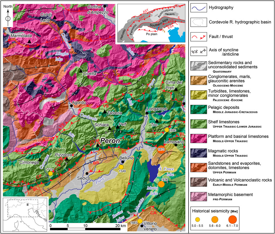
FIGURE 1. Simplified geological map of the Alpine sector where the study area (Mt. Peron) is located. List of acronyms: BL: Belluno thrust; BS: Belluno syncline; and CVM: Val Carpenada-Val di Vido-Val Madonuta thrust. The major historical earthquakes that occurred in the area are reported, along with their reconstructed magnitude (Mw) (source: Rovida et al., 2022).
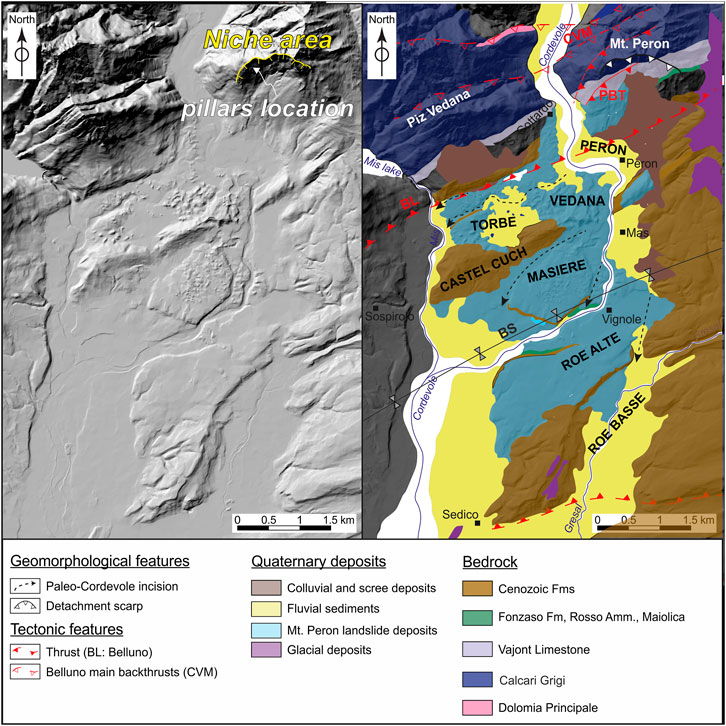
FIGURE 2. Shaded relief model (left) and geological map (right) of the study area. BL: Belluno thrust; BS: Belluno syncline; CVM: Val Carpenada-Val di Vido-Val Madonuta thrust; and PBT: Peron back thrust (modified after Rossato et al., 2020).
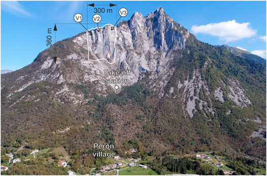
FIGURE 3. Aerial view of the Mt. Peron niche (view from the south); the area included in the virtual outcrop, south-facing and near-vertical with its dimensions, the take-off location of the UAV, and the three rock pillars analyzed by means of the distinct element method (V1 to V3) are also indicated.
Geomorphologically, the study area is located in the Piave river valley, 10 km west of Belluno, in a tract of the river valley that has been deeply modified by glacial advances during the quaternary, with the Piave glacier up to 800 m thick (Pellegrini et al., 2006). The Cordevole river is a tributary of the Piave river and crosscuts the study area. This is a typical mountain stream, 79 km long, with a catchment surface area of about 830 km2, an elevation ranging from ca. 2,000 to 275 m a.s.l. and a mean annual rainfall of ca. 1,500 mm. It crosses the Venetian Dolomites and passes in between the Piz Vedana (1,324 m a.s.l.), to the west, and the Mt. Peron (1,486 m a.s.l.), to the east. When the Cordevole river reaches the plain, it starts flowing on the rock avalanche deposits, cross-cutting them with an overall north-east/south-west path and a ca. 1% gradient. Locally, the river flows into meanders eroded into bedrock, probably reusing an ancient bed, older than the rock avalanche (Rossato et al., 2020). Some younger paleo-channels ascribable to the Cordevole river can be recognized across the rock avalanche deposits, suggesting that multiple river avulsion occurred after the event, prior that the river encased in its current bed (Figure 2).
From the seismotectonic point of view, the area experienced several moderate earthquakes in the last centuries (e.g., in Jun. 29, 1873, Alpago event, Mw 6.29, Io IX-X MCS and in Nov. 18, 1936, Alpago–Cansiglio earthquake, Mw 6.06, Io IX MCS; Rovida et al., 2020, 2022; Figure 1) reaching intensity values up to VII-VIII (MCS). Earthquakes are a common trigger event for rockfalls in this region, where large past events have been possibly associated with a dynamic triggering in historical and pre-historical times (e.g., Rossato et al., 2018, 2020; von Wartburg et al., 2020).
Dataset and Methods
Data Acquisition
In order to take advantage of a refined 3D view of the study area, we have performed a photographic coverage of the Mt. Peron niche area through a drone flight.
We used a DJI Phantom 4 Pro Plus multi-rotor UAV (unmanned aerial vehicle) equipped with a built-in high-resolution camera. The built-in lens has a field of view of 84° with a focal length of 8.8 mm/24 mm (35 mm equivalent focal length). The camera is equipped with a 1" 20 MP CMOS sensor, and we recorded photographs in RAW format; all the photographs were manually shot with the drone hovering.
We chose to model the three major pillars visible in the niche area (Figure 3), considering that these are the most hazardous features for potential instability. It is noteworthy that the niche area presents an elevation drop of ca. 500 m with an almost vertical rock wall. It is an inaccessible site and remote sensing is the most important data source for this case study. A total of 145 photographs (Figure 4A) were shot following a parallel-axis shooting strategy with the addition of a grid of oblique photographs, especially for the upper sector, where complex rock dihedra are present. Photographs were processed in RAW format and were acquired from 50 to a maximum of 200 m from the target surface, with most of the images shot at ca. 100 ± 50 m. We obtained an optimal overlapping of the photographs for the 3D model building, with the modeled area covered by at least nine photographs for each sector of the point cloud (Figure 4B).
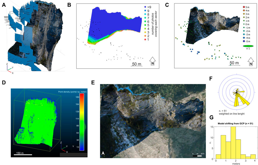
FIGURE 4. (A) Modeled virtual outcrop with the location of the acquired photographs from UAV; (B) coverage of the point cloud, view from above; (C) accuracy of the relative position of cameras as calculated from geotagged photographs and relocated after structure from motion calculations; (D) 3D dense cloud point density (nr. points/sq. meter); (E) comparison of the virtual outcrop georeferencing with an orthophoto coverage from aerial imagery (25 cm of resolution, courtesy of Veneto Region): shifting from a set of visually selected GCPs (n = 51) is reported in the map (yellow arrows; the length of each arrow indicates the amount of shifting); (F) direction of shifting and (G) its amount is also shown.
Point Cloud Generation
We used the SfM photogrammetry software Metashape (Agisoft, 2022) to produce a 3D point cloud from the UAV photography. The camera alignment was obtained; thanks to the co-registration of 81,306 tie points, and the internal accuracy of the model was tested over 16 control points manually checked over the different photos, with an RMS reprojection error of 0.189 m. The dense point cloud was built without down-sampling of the original images (i.e., ultra-high-quality setting in Metashape) and with a mild depth filtering.
We were not able to position ground control points (GCPs) on the site due to the inaccessibility of the surveyed cliff. We then relied on the direct georeferencing of the model by means of the photographs’ geotagging, as recorded by the built-in navigation—grade GNSS receiver. We are aware that this is a source of uncertainty in the model reconstruction; so, after the point cloud generation, we analyzed the accuracy of the model positioning through an ex-post 2D validation approach. We provided an estimate of the accuracy in the absolute georeferencing of the virtual outcrop by comparing the orthophoto derived from our virtual outcrop with a high-resolution orthophoto-mosaic derived from an aerial coverage of the area from the Veneto Region (AGEA 2015; last accessed in 2022; courtesy of Veneto Region). The reference orthophoto coverage has a nominal resolution (GSD) of ca. 30 cm (specifically 50 cm in mountain regions and 20 cm in plain sectors).
Fracture Measurement on the Virtual Outcrop
For fracture digitizing and orientation measurements, we used the CloudCompare software (CloudCompare, 2022). CloudCompare is a non-commercial processing software for 3D point clouds and meshes and is available under the GNU General Public License. It includes many functionalities and is widely used for its versatility and the availability of many science-oriented plugins developed by the user community. We performed data digitization through the plug-in Compass (Thiele et al., 2017) which provides an assisted interpretation procedure for linear fracture detection. Planar surfaces can be directly measured on the point cloud, if well exposed, by clicking on the fracture surface; the calculated orientation is the best-fitting planes passing through the points included in the circular window around the clicked point. Alternatively, the estimation of the structure orientation is based on its intersection with a non-flat surface (i.e., the virtual outcrop surface). Linear traces of discontinuities on the virtual outcrop can be digitized in CloudCompare by manually selecting the points including the discontinuity trace. Then, a computer-assisted procedure helps in selecting all the points in the cloud connecting two near points. The software uses a least-cost-path algorithm to follow these discontinuity traces along the surface between the user-defined start and end points and then calculates the best-fitting plane to estimate the orientation. The least-cost-path procedure, applied on points included in a spherical search, is based on user-defined scalar values, associated with each point in the cloud (e.g., color similarity, brightness, or presence of high-curvature regions—edges). We, here, adopted an approach based on the brightness of the points (i.e., the absolute value of the associated color in a greyscale rendering), since fractures are visually associated with hairline shadows in the acquired images. Finally, once the fracture trace on the modeled surface is defined (Figure 5), the best fitting plane is calculated (i.e., the plane where most of the points on the fracture lie) together with its orientation (i.e., dip direction and dip).
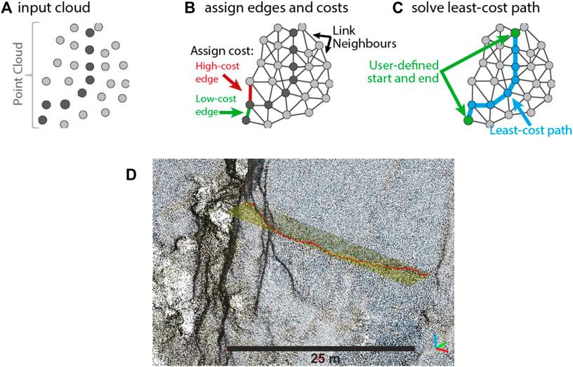
FIGURE 5. Schematic representation of the least-cost-path approach to trace detection for point clouds (modified after Thiele et al., 2017). In this example (A), points on the discontinuity trace have a lower brightness value (dark grey); (B) the brightness-based cost function results in low-cost edges between neighbor points that fall on the structure trace (dark grey); (C) a least-cost-path calculation provides an estimate of the structure trace among user-defined start and end points of the discontinuity; and (D) example of a fracture trace digitized in Compass plugin for CloudCompare: the fracture plane (in yellow) has been calculated from the best fitting of the traced fracture on the surface of the point cloud (in red).
Alternatively, if most of the detected points of the fracture trace are almost collinear and the best-fitting plane is not adequately constrained, the fracture can be manually digitized by selecting only three points of the fracture and proceeding with the classical solution of the three-point problem.
Finally, poles to fracture planes are statistically analyzed in order to calculate the average orientation of each fracture. For this statistical analysis, we used the software Wintensor v.5.8.8 (Delvaux and Sperner, 2003). First, we clustered the poles to the fracture planes through a K-means algorithm (MacQueen, 1967): the number of clusters is fixed a priori by the operator, and the calculator finds the centroids of the clusters that minimize the total intracluster variance and maximize the intercluster distance. A number of clusters were fixed with a visual inspection of the data, aided by density contouring of fracture poles. The output includes the orientation of the fracture sets, the Fisher’s dispersion factor (i.e., K value, Fisher, 1953), and the mean cone angle (MCA) enclosing the data distribution.
Stability Analysis: Distinct Element Numerical Simulations
To evaluate the stability of the three rock pillars under investigation, the distinct elements method (DEM) was used (Cundall and Strack, 1979). This method is widely used to simulate static and dynamic problems involving dry or wet granular media of any size and shape (Gabrieli et al., 2013), from powders (Martin et al., 2003) to sands (Gabrieli et al., 2009), gravels, and fractured rock masses (Spreafico et al., 2016; Calvetti et al., 2019). Each body is treated as a distinct rigid element having six degrees of freedom, and it communicates with the other bodies through specific contact laws. The algorithm is explicit and solves the equations of motion of all bodies in the time domain for both translation and rotation through a finite difference integration scheme.
At each time step: i) the list of contacts between the various blocks is updated, ii) each contact provides a normal and tangential force that is transferred to the center of mass of each block, iii) the body forces and possibly other external forces are added to the resulting force, and iv) the positions and velocities of the blocks are updated, integrating over time.
In this case, the method is particularly suitable for the intrinsically fractured nature of the rock mass along predefined planes and for the ability to manage multiple contacts, fractures, and detachment problems between the blocks, even with large deformations.
The complexity of the rock mass and the three prisms and, above all, the presence of the joint planes (that will be called K1), which are oblique with respect to the other three (K2, K3, and S0), made it necessary to use a 3D numerical modeling. Moreover, the presence of several sub-vertical bedding planes (called S0) means that these three pillars cannot be assimilated to three non-fractured blocks that detach but rather to a cluster of adjacent blocks that could potentially detach, slide, and overturn.
The software used for this analysis is 3DEC by Itasca (v. 5.2, 2016; Itasca, 2016), which can generate polyhedral 3D blocks starting from the deterministic and statistical description of the planes that delimit them (Discrete Fracture Network—DFN). It also internally implements a method for evaluating the safety coefficient of the rock mass, similar to the strength reduction method used in finite element codes.
Results
3D Model Generation and Discontinuity Measurements on the Virtual Outcrop
By means of the SfM-VsM workflow, we obtained a sparse point cloud from camera alignment with a mean key point size of 2.2 pixels, a maximum reprojection error of 0.56 pixels, and a mean tie point multiplicity of 8.5. The estimated relative accuracy in the camera position has been evaluated through an application of the Metashape software, and we found an average accuracy of 1.5 m (Figure 4C). The dense point cloud, calculated using the MvS processing, consists of 149,814,051 points, after trimming, with an average spacing of ca. 5 cm (Figure 4D).
We performed a 2D georeferencing to check if the positioning errors were mainly due to shifting and/or tilting or an internal deformation of the model. This procedure is a simplification of a real 3D georeferencing of the model but, since accurate GCPs are not available, it still constitutes an exploration tool that can provide the relative distribution and orientation of errors projected on a horizontal plane. The accuracy of a zero-order shift (i.e., a simple shift on the horizontal plane) was 5.65 m and of a second-order transformation (i.e., implying internal deformation of the model) of 3.18 m. Conversely, assuming a first polynomial transformation (i.e., implying shift scale and rotations only), we obtained a root mean square error of 1.47 m (a maximum error of 4.83 m), with greater errors aligned along the y-axis. We can thus assume that the 3D georeferencing of the virtual outcrop can suffer from small misorientations, especially around the x-axis of rotation, but also those internal distortions are not the main source of error. If we assume that internal distortions are relatively small and consider the maximum error (4.83 m) as due to the model misorientation, this will result in ca. 1–2 degrees of orientation errors for fractures as large as those digitized in the outcrop (i.e., tens of meters long).
Considering that our scope is to perform a first-order stability analysis of a rock cliff where no other detailed measurements are available, we, here, assume that the estimated error is small enough to be accepted for the successive analysis.
On the virtual outcrop, we measured 159 discontinuity planes that have been clustered into four sets of fractures (i.e., S0, K1, K2, and K3; Figure 6; Table 1) with 18 data resulting as non-classified. The first cluster, S0, represents the bedding, corresponding to sub-vertical planes striking ca. WSW-ENE and located in the forelimb of the anticline, in the hanging wall of the BL thrust. The cluster K1 represents a principal sub-vertical fracture system, NW-SE-striking, that cuts through the bedding and, together with S0, isolates the main pillar and rock prisms on the analyzed wall (Figure 6C). Clusters K2 (NE-SW striking high-angle fractures) and K3 (low-angle to sub-horizontal planes) represent two secondary and less pervasive discontinuity systems.
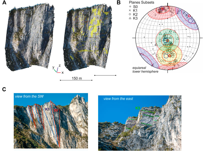
FIGURE 6. (A) Dense point cloud of the virtual outcrop and measured fracture planes (in yellow); (B) stereoplot of the clustered data (poles to planes) with the resulting mean orientation of each cluster (red small circles), mean cone angle (red continuous line), and the external limit of each cluster (red dashed line); and (C) UAV-based imagery of the niche area with illustrative fracture sets is highlighted.
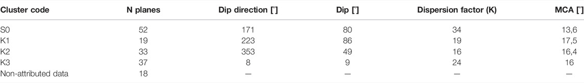
TABLE 1. Orientation and dispersion factor (K) for the recognized fracture planes and mean cone angle (MCA).
The four detected fracture sets have been compared with field-based measurements, taken at the base of the rock cliff and along a rappel descent on the same sector of the three pillars and during a field survey in areas close to the sides of Mt. Peron (Figure 7).
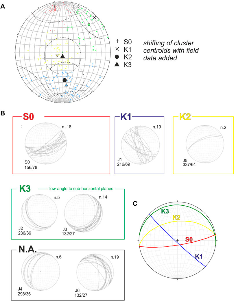
FIGURE 7. Ground truthing of structural data and additional field data. (A) Data clustering is re-calculated after adding the field data, cluster mean orientation, and mean cone angle from the virtual outcrop alone are reported in black, new data clustering and mean orientation is color-coded; (B) discontinuity grouping after De Zorzi (2013) and Rossato et al. (2020) (sets J1 to J6 after their original coding) and bedding orientation (S0) measured in situ along a transect surveyed through a rappelling descent: an attribution to our clusters is proposed, and N.A. stands for non-attributed data; and (C) reference for the orientation of average sets as calculated in this study.
Field-measured fracture sets were coded as S0 (for bedding) and as J1 to J6 classes. Our clusters S0 and K1 from the UAV survey show good agreement with S0 and J1, respectively (Figure 7).
3D Geometry Reconstruction of the Three Pillars and of the Discrete Fracture Network
The point cloud of the rock mass obtained through the SfM-VsM workflow was used to describe in a simplified way the external surface of the rock mass in the DEM model (Figure 8A). It should be noted how a higher detail in the description of the model surface has no benefit in this analysis: the three prisms are quite big (the smallest is 100 × 15 × 20 m) and almost regular and higher detail of the surface would be functional to the stability analysis of detachment of the smallest blocks (metric and sub-metric) but not to an overall stability analysis; moreover, it would greatly increase the computational cost of the model. On the contrary, more detail is needed in the definition of the joints because they affect the level of fracturing of the rock mass and have a great impact on the stability analysis.
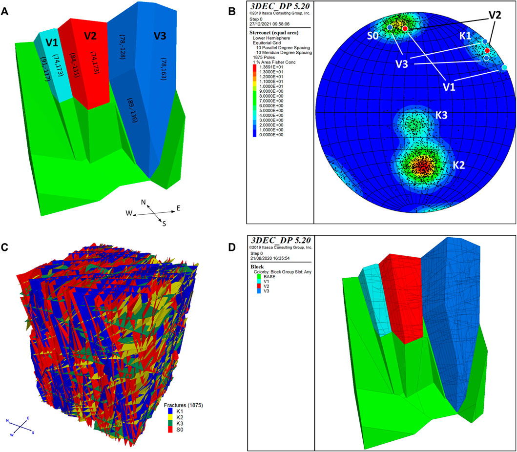
FIGURE 8. (A) The layout of the simplified geometrical model with the indication of some face orientations (dip and dip direction) of the three pillars; (B) stereonet of the modeled DFN with the poles of the external surfaces of the three pillars superimposed; (C) three-dimensional DFN model with the four sets of discontinuities; and (D) the three pillars with the joint sets.
First, the planes delimiting the three prisms from the rest of the rock mass have been added (namely S0 on the backplane and K1 and K2 for the other sides). The rock mass behind and at the base is assumed to be stable and fixed in the model. Subsequently, the measurements on the joints coming from the virtual and conventional discontinuity mapping have been used to create a DFN. For this purpose, we used WinTensor and the DFN module of 3DEC by Itasca (v.5.2, 2016; Itasca, 2016). We adopted a probabilistic joint orientation according to a Fisher distribution (Fisher, 1953) with a dispersion factor k calculated on the outcrop data (Table 1). For the fracture size distribution, we assumed circular fractures of finite size following a power law with a scaling exponent equal to 3.2 (Priest and Hudson, 1981; Priest, 1993; Bonnet et al., 2001). The density of the joints was expressed as p10, in terms of the number of fractures per unit of length; alpha was estimated along three scanlines in the point cloud. In 3DEC, fractures of the DFN have been generated until a target value of p10 is reached for each joint set. Although as evidenced by other authors (Elmo and Stead, 2010; Dershowitz et al., 2014), other parameters such as the areal intensity (p21) or the volumetric intensity (p32) can provide a more realistic description of the fracture density of the rock mass, considering the fairly regular shape of the pillars with some faces parallel to the joint planes, we decided to use the p10 value as the DFN generation parameter, taking care to choose scanlines orthogonal to these faces and thus maximizing its information content.
The final DFN model with the four discontinuity sets S0, K1, K2, and K3 used in the simulations is depicted in Figure 8C while their orientations with the poles of the external surfaces of the three pillars superimposed are represented in Figure 8B. Note how the three pillars share the same orientation of the south-facing face, almost parallel to the bedding plane S0, while the other subvertical surfaces confining the three dihedrals belong to the K1 plane subset. This particular fairly regular configuration of the three vertical prisms being analyzed, with these two well-exposed surfaces forming an angle between 70° and 55°, has allowed a sufficiently detailed statistical reconstruction of the families of the internal joints.
For the constitutive model of the joints, a generalization of the Mohr–Coulomb shear strength envelope was also assumed with a normal tensile limit value while rock blocks were simulated as non-deformable bodies having a unit weight of 25.5 kN/m3. The mechanical parameters used in the model were estimated based on the field measurements obtained by Di Giusto (2012) and from samples taken at the toe of the vertical slope. The same parameters were, therefore, extended to the other three pillars under investigation. The joint compressive strength was estimated with the Schmidt hammer (Deere Miller, 1966; Aydin, 2008) while the RQD index was determined from the density of joints (Palmström, 1982). Spacing conditions of discontinuities and groundwater conditions have been estimated quantitatively and qualitatively by geol. Di Giusto during the field survey, providing a final RMR estimate of 58 (Barton 1974; Bieniawski, 1989). On the basis of additional sclerometer tests and roughness measurements in the niche at the toe of the first pillar on weathered and unweathered rocks, the shear strength of joints was evaluated according to Barton and Choubey (1977). The basic friction angle was assumed to be equal to 32° for this rock type. The cohesion value attributed to the joint planes usually takes into account several aspects including the real cohesion of the intact rock and the fraction of the rock bridges on these surfaces (Jennings, 1970; Calvetti et al., 2019). In the absence of this information, we decided to quantify the joint cohesion by carrying out a small stability analysis on the large rock slab of known volume, placed at the top of the biggest pillar and adhered to the sub-vertical wall, with a procedure similar to that reported by Sampaleanu (2017). In fact, for this high-slope configuration, the friction angle of the joint plays a marginal role compared to cohesion and allows a better evaluation of the latter. It has also been hypothesized that this value maybe the same in the joints of the other pillars. This assumption represents a precautionary estimate of the real cohesion value since it is likely that the bedding plane S0 on which the stability of the slab was evaluated represents the plane with the greatest degree of alteration and lowest normal stress and therefore the lowest cohesion value. Due to the difficulties in getting samples and the lack of other specific geomechanical tests, the joint stiffnesses were not calculated, but realistic values have been assumed according to literature (Fairhurst, 2014). We used a fairly low value to compensate for the rigid block assumption and the reduction of joint stiffness for tension mechanisms which is expected for subvertical joints. In any case, it must be recalled that the stiffness of the joints has little or no influence on the evaluation of the safety factor which is instead greatly influenced by the strength parameters (Wines, 2020).
The values reported in Table 2 are therefore assumed for the joints.
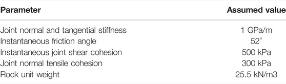
TABLE 2. Numerical parameters for the mechanical description of the rock and of the joints in the distinct element model.
For the evaluation of the stability of the rock mass, the strength reduction method, which consists in looking for the shear resistance reduction factor of the joints (friction angle and tangential cohesion only) that leads to the limit equilibrium condition (Matsui and San, 1992), was adopted. The calculation started by applying gravity with a fictitious high joint shear strength and reaching a stable condition. After that, the joint properties were updated, and a bracketing approach was used in the factor of safety calculation by narrowing step by step the factor span between a stable and unstable solution (Dawson et al., 1999).
Stability Numerical Analysis
The stability analysis was performed on each of the three pillars separately, i.e., by fixing two pillars each time and solving the equilibrium of the remaining one.
The factor of safety (FOS) and its associated instability mechanism were assessed for each pillar to identify those in more precarious conditions and not to evaluate a safety factor in an absolute sense.
It is emphasized that the simplifications introduced in the model (e.g., the assumption of rigid blocks, the discontinuity planes imposed with the DFN, and the parameters calculated as lower limits) do not allow a refined numerical analysis but to determine on which pillars to focus attention for further surveys. It should be noted that, for a generic FOS greater than 1, the corresponding instability mechanism is obtained by dividing the tangent of the friction angle of the joints and the shear cohesion by the same FOS and observing the kinematics of the blocks in these conditions. The displacements obtained with this method are, therefore, not the real displacements of the mass but highlight the type of rupture mechanism. The smallest pillar (V1) showed a stable condition with a FOS = 1.6 associated with a planar sliding instability mechanism and a tendency to overturn toward the south-east partially sliding on the bedding plane (Figure 9A).
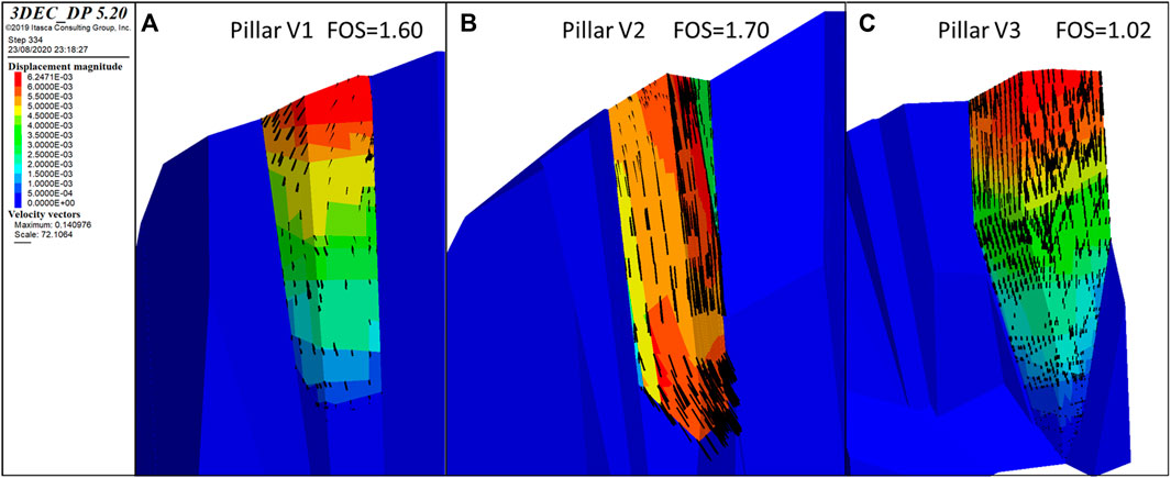
FIGURE 9. Results of the stability analysis of the three pillars in the niche; failure mechanism (displacement and velocity vectors), together with the calculated factor of safety (FOS) for each of the three pillars are indicated. (A) Pillar V1, (B) Pillar V2, (C) Pillar V3.
The intermediate pillar V2 has a safety factor of 1.7, slightly higher than the first. This result can be explained by the fact that despite having a height similar to the smallest one but a width approximately double the bedding plane, it has the surface facing south-west and orthogonal to the bedding with a lower dip value (84° instead of 90°), and therefore, overall, a center of mass that makes the pillar more stable. The failure mechanism, in this case, is of the sliding type on the bedding plane with partial rotation at the toe (Figure 9B).
Finally, the last pillar V3 has a safety factor of just above unity (FOS = 1.02). Its southeast face has a slope angle on average higher than the other two prisms (78° instead of 73°) and more than the bedding dip. This is also evidenced by the 30 × 40 × 3 m prismatic rock slab, slightly bent at the base, that appears to be suspended on its top (Figure 10) and that was used for the calibration of the joint cohesion. Even removing these slabs having a considerable thickness and whose stability is mostly controlled by the joint cohesion, the safety factor remains low, and the mechanism is a complex failure controlled by the S0 bedding surfaces (Figure 9C). This can be explained by the particular geometry of the base of the prism which has an external surface with an inclination close to the vertical (88°) (Figure 10). The precarious conditions of this huge pillar are also confirmed by the evident detachment of blocks in recent times, as highlighted by the weathered rock surfaces at the foot.
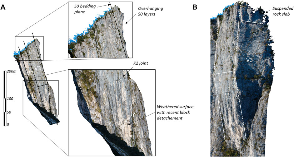
FIGURE 10. (A) Lateral view of the three pillars from the south-west with details of the top and the bottom part of the V3 prism; (B) perspective view of the V3 pillar geometry with the suspended rock slab (view from the southeast).
Discussion
The measured fracture sets, well-fitting with the few available field measurements, can be interpreted considering the geological setting of the area and their possible role in promoting the rock volume instability. The subvertical NW-SE trending fracture planes (K1–J1), well represented in the volume, can be tentatively ascribed to inherited structures subparallel to the local margin of the Trento platform (Costa et al., 1996), later reactivated during the Alpine (or Dinaric) orogeny, as tear faults in the hanging wall of the BL thrust.
J2 and J3 are low angles to subhorizontal fractures (Figure 7). The K3 set in the virtual outcrop does not include south-dipping fractures, suggesting that either the fractures are too small to be imaged (i.e., hairline fractures with a submillimeter aperture) or, alternatively, these two sets are not present in the investigated area. This mismatch could be ascribed to rotations of low-angle fractures by a small amount of progressive folding of the BL thrust hanging wall anticline or by a zonation of the fracture distribution with respect to the anticline itself. Ground-measured J4 and J6 sets (i.e., moderately dipping fractures) are partially represented by our non-attributed data (10 out of the 18 measures). A further classification, forcing the K-means algorithm to six classes, would potentially recognize all these sets.
Finally, clusters K2 can be representative of the BL thrust (J5 in Figure 7A) planes with some differences detectable in the plane direction.
Figure 11A highlights the fractures responsible for past but undocumented collapses of the pillars. Bedding (S0) and K1 planes isolate rock slabs, whose first slipping may possibly occur along the back thrust (at the base) and S0 planes. After this, tensile failure of the other joints occurs. Slipping off the slabs seems thus to be the dominant failure mechanism. Traces of those detachments are shown in Figure 11A, where clean exposed surfaces are visible along K1 surfaces.
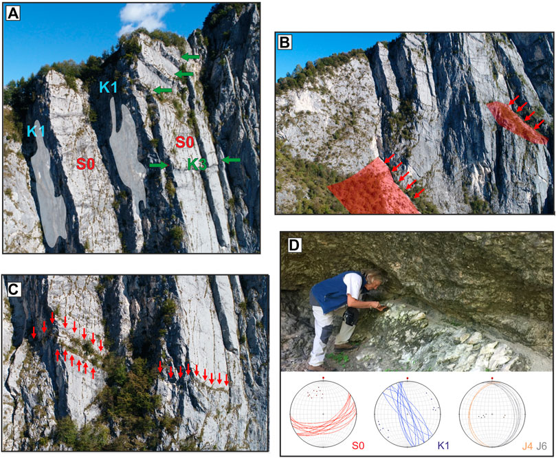
FIGURE 11. (A) Subvertical bedding planes (S0) and fractures (K1) are well recognizable in the pillars area and together with K3 fractures isolate rock dihedra potentially prone to failure; note the whitish faces of K1 fracture planes (highlighted) indicating a recent detachment of rock slabs; (B) south-dipping planes ascribable to shear planes of the Mt. Peron back thrust PBT (main planes are highlighted in red); (C) subhorizontal and low-angle fractures deeply weathered and affected by karst phenomena; (D) karst cave in the SE side of Mt. Peron (“Sass Taja” locality) and structural data surveyed.
The investigated area of the niche does not present clusters of fractures representative of the PBT whereas field surveys performed at the base of the cliff recognized well-expressed fault planes possibly connected with this structure (Figure 7B). Conversely, the back thrust is visible through land survey, and it defines the slipping plane visible at the base of the pillars (Figure 3).
The field surveys performed in the niche area and on the northern flanks of Mt. Peron as well, pointed out the presence of intensive karst formation in the Mt. Peron area, especially along K2 and K3 fracture planes, and secondarily along S0 and K1 (Figures 11C, D).
The two sub-vertical sets, mostly S0 and K2, create a preferential path for water infiltration. The presence of sub-horizontal planes (K3) cutting the principal sets can create significant water stagnation after meteorological events, allowing a low water outflow because of the karst formations. Mainly, K3 sub-horizontal fractures present a fine-grained filling material causing water stagnation and enhancing the weathering of fracture surface. The rock weathering and production of filling material are surely worsened by freeze-thaw cycles in the outermost part. Figure 11C, shot by the UAV during the aerial survey, shows a detail on the lower part of the pillars where a major fracture, belonging to K3, is filled with crushed material and is particularly highlighted by a vegetation line. Figure 11D shows an example of the karst formations surveyed in the Mt. Peron area. This outcrop is located on the eastern side of the mountain (locally called “Sass Taia”) and exposes a cave ca. 2 m high and 6 m long. Here, the bedding (S0) and a set of K1 fractures (i.e., the most frequent sub-vertical fracture system) are pervasively dissecting the rock volume. The planes J4 and J6, measured during field surveys, are possibly secondary discontinuities, linked to the main low-angle shear zone (BL thrust).
From a methodological point of view, the photogrammetric survey performed with UAVs was revealed to be an extremely valid alternative, in terms of data reliability, effectiveness, and flexibility from an observation perspective, in comparison to ground-based scanning systems (e.g., terrestrial LiDAR) and can be used to integrate field-based data collection. In our case study, we only suffered from limits on the maximum altitude reachable by the UAV due to strict law regulations in Italy.
The main shortcoming in the data accuracy can be recognized in the use of low-accuracy GNSS positioning for the direct georeferencing of the model.
The most promising results in the direct georeferencing method can be obtained using a drone with a built-in survey-grade GNSS real-time kinematic receiver (RTK-UAV). Still, with this setup and under optimal conditions, the vertical accuracy is 2–3 times greater than the horizontal one, leading to elevation discrepancies of ca. fivefold the ground sampling distance (Hugenholtz et al., 2016; Forlani et al., 2018). This leads to the consideration that for accurate results at the sub-metric scale, the use of GCPs is still mandatory and their number and spatial distribution had to be accurately planned for avoiding unintended induced deformations in the model (Sanz-Albanedo et al., 2018). Nonetheless, for low-resolution modeling (i.e., at the metric scale), alternative approaches can be considered if provided with an evaluation of the georeferencing accuracy.
A similar approach has been applied for evaluating the stability of rock cliffs with very limited or irregularly distributed GCPs (Mancini et al., 2017) or without any GCPs (e.g., Wang et al., 2019), providing an estimate of the georeferencing accuracy and internal model accuracy. Meinen and Robinson (2020) demonstrated that in the case of the absence of GCPs, the coupling of orthogonal and oblique imagery led to the highest checkpoint accuracy in both the vertical and horizontal dimensions. The same considerations were also drawn by Jaud et al. (2019), who, consistently with our workflow, suggested optimizing the optical camera model and/or the processing strategy to improve the quality of the resulting model.
We here underline that in some applications, e.g., for fast data acquisition and mapping during emergency response or for mapping of inaccessible sectors, the accuracy of direct GNSS/INS observation can be enough if the required accuracy is not at sub-metric quality (e.g., Zhou 2009; Pfeifer et al., 2012; Nex and Remondino, 2014).
The detail of the obtained points cloud is sufficient for measuring joints and fracture planes at the observational scale and led us to obtain hundreds of measures in a few hours of workstation work.
On the other hand, working on a virtual outcrop prevents any direct measurement of the fracture aperture or conditions (e.g., filling and aperture weathering degree). In order to obtain a density of the point cloud reliable for fracture detection, an area of ca. 105 m2 can be covered by a single survey, limiting the area that can be investigated and possibly resulting in partial views or representations of the real distribution of fracture sets.
In our case, in particular, the measurements ascribable to the PBT back thrust were only surveyed in a representative number during field surveys due to the limited spatial distribution of this set of discontinuities.
For what concerns the numerical analysis, assuming a dominant mechanism of structural controlled instability, it was performed with great detail on the determination of the 3D orientation of the fracture planes obtained from the virtual outcrop and using instead a simplified model as regards the overall shape of the three pillars. This made it possible to carry out a 3D DEM analysis without increasing the calculation time too much and, at the same time, maintaining an excellent level of detail in the results. On the contrary, the inaccessibility of the rock face did not allow a more accurate evaluation of the mechanical parameters of the rock mass which would have allowed the attribution of specific mechanical properties to each family of joints. The real consistency of the rock bridges and, therefore, a better calibration of the joint parameters can be carried out through a back analysis of blocks that will detach in the future as described, for example, by Bonilla-Sierra et al. (2011). For this reason, the safety coefficient of every single pillar should not be considered a value that certifies its intrinsic stability but rather a parameter of comparison with the stability of the other pillars. To assess rockfall hazards, the detailed characterization of rock masses is a priority objective not only for the Mt. Peron niche area but for the whole Southern Alps, where a relatively high density of population (especially tourists) is exposed to highly dynamic geological processes. This is especially true if we consider that hazard from moderate rockfalls events diffusively characterizes a large part of the territory and can be potentially triggered even by moderate ground motions (i.e., V degree of the ESI07 Intensity Scale; Michetti et al., 2007), quite frequently hitting the area. Recent examples are the deadly rockfall in Bolzano Province (Jul. 17, 2001), triggered by a moderate M 5.2 event in Merano, or the rockfall that destroyed a house in Clibbio (BS), triggered by (Nov. 24, 2004) Salò earthquake (M 5.2; Michetti et al., 2005; Viganò et al., 2018).
Conclusion
In this work, we performed a UAV-based photographic survey of the niche area of the Masiere di Vedana rock avalanche. By means of an SfM and MsV approach, we obtained a dense point cloud and took geo-structural measurements on the obtained virtual outcrop. We then used these orientation data to populate a DEM model of the rock volume and to run numerical simulations of the stability of three main pillars in the area under investigation.
The main findings and some additional considerations on the results can be summarized as follows:
- Four main discontinuity sets can be defined in the analyzed rock volume. The sets are closely related to the tectonic deformation history of this rocky wall and to the development of secondary structures related to the main tectonic lineaments.
- There is a good consistency between measurements taken on the virtual outcrop and the field-based ones. Nevertheless, we observed some significant mismatching. Uncertainties can arise from three main sources. The first is the very limited number of field-based measurements (some field-based sets are populated by less than five elements). The second reason is due to the internal deformation of the virtual outcrop, which was not corrected with ground control points characterized by cm-scale accuracy. We discussed the weaknesses of our reconstruction, and the accuracy in the model looks reasonable, but we cannot exclude inaccuracies. Finally, some field measurements were taken at the very base of the rock cliff, where our model lacks exposure and vegetation is present; we could also infer that some sets have a spatially limited distribution, being distributed only in specifically oriented zones of the rock volume.
- The presence of joints with a fairly regular orientation and a fairly regular conformation of the pillars suggests a structurally controlled instability mechanism which was evaluated using a rigid block DEM numerical model. Assuming that the joint parameters are the same in the three pillars, the numerical model suggests that the third pillar (V3) is in more precarious conditions. This is confirmed by some precursor signs of detachments at the base. In the present conditions, not being able to easily reach the rock wall to carry out geomechanical tests on the joints and the intact rock, this result represents the best possible risk assessment. A more accurate analysis that considers potential brittle rock mass failures can be initiated by being able to focus attention on the most unstable pillars and launching a further series of investigations on the mechanical properties of the rock mass. Recurrent rockfalls take place frequently along the southern side of Mt. Peron, as testified by newspaper records and technical reports (e.g., Di Giusto, 2012). Luckily, these detachments involved small rock volumes and did not cause any damage but, on the other hand, suggest the lack of equilibrium in the rock mass. As occurred in various other cases (e.g., the Termeno rockfall, in the Bolzano Province, Italy; Martin et al., 2020), landslides may occur in the same place as older events. The potential impact of a rockfall on the village nearby is a major source of hazard and, according to the writers, should be further investigated and the cliff monitored.
Data Availability Statement
The raw data supporting the conclusion of this article will be made available by the authors, without undue reservation.
Author Contributions
FL conceptualized the work, built the 3D model, and provided accuracy estimates; FB and FG ran the stability analysis of the rock pillars; FB digitized the fractures and the virtual outcrop and made the statistical analysis; RG shot the photographs from the UAV and provided technical assistance; and SR, AM, and SM framed the work, provided field data from ground truthing and financial support to this research. All the authors contributed to writing the manuscript and reviewing the work.
Funding
All the work has been done with research funding by AM and SM.
Conflict of Interest
The authors declare that the research was conducted in the absence of any commercial or financial relationships that could be construed as a potential conflict of interest.
The reviewer FPM declared a shared affiliation with the authors RG and AMM to the handling editor at the time of review.
Publisher’s Note
All claims expressed in this article are solely those of the authors and do not necessarily represent those of their affiliated organizations, or those of the publisher, the editors, and the reviewers. Any product that may be evaluated in this article, or claim that may be made by its manufacturer, is not guaranteed or endorsed by the publisher.
Acknowledgments
The authors want to thank Itasca Consulting Group for a loan of the 3DEC software within the Itasca Education Partnership (IEP).
References
AGEA (2015). Available at: https://idt2.regione.veneto.it/gwc/service/wmts.
Agisoft (2022). Available at: https://www.agisoft.com (last accessed December, 2021).
Aydin, A. (2009). ISRM Suggested Method for Determination of the Schmidt Hammer Rebound Hardness: Revised Version. Int. J. Rock Mech. Min. Sci. 46, 627–634. doi:10.1016/j.ijrmms.2008.01.020
Barton, N., Choubey, V., and Beniawski, Z. T. (1977). The Shear Strength of Rock Joints in Theory and Practice,” in Rock Mechacnics. , 10. New York: Wiley Engineering Rock Mass Classifications, 1–54. doi:10.1007/BF01261801
Barton, N., Lien, R., and Lunde, J. (1974). Engineering Classification of Rock Masses for the Design of Tunnel Support. Rock Mech. 6 (4), 189–236. doi:10.1007/bf01239496
Bonilla-Sierra, V., Scholtès, L., Donzé, F. V., and Elmouttie, M. K. (2015). Rock Slope Stability Analysis Using Photogrammetric Data and DFN-DEM Modelling. Acta Geotech. 10, 497–511. doi:10.1007/s11440-015-0374-z
Bonnet, E., Bour, O., Odling, N. E., Davy, P., Main, I., Cowie, P., et al. (2001). Scaling of Fracture Systems in Geological Media. Rev. Geophys. 39 (3), 347–383. doi:10.1029/1999RG000074
Calvetti, F., Frenez, T., Vecchiotti, M., Piffer, G., Mair, V., and Mosna, D. (2019). DEM Simulation of the Evolution of an Unstable Rock Face: A Modelling Procedure for Back Analysis of Rockslides. Rock Mech. Rock Eng. 52, 149–161. doi:10.1007/s00603-018-1576-0
Cawood, A. J., Bond, C. E., Howell, J. A., Butler, R. W. H., and Totake, Y. (2017). LiDAR, UAV or Compass-Clinometer? Accuracy, Coverage and the Effects on Structural Models. J. Struct. Geol. 98, 67–82. doi:10.1016/j.jsg.2017.04.004
CloudCompare (2022). 3D Point Cloud and Mesh Processing Software Open Source Project. Available at: https://www.danielgm.net/cc/.
Cook, K. L. (2017). An Evaluation of the Effectiveness of Low-Cost UAVs and Structure from Motion for Geomorphic Change Detection. Geomorphology 278, 195–208. doi:10.1016/j.geomorph.2016.11.009
Costa, V., Doglioni, C., Grandesso, P., Masetti, D., Pellegrini, G. B., and Tracanella, E. (1996). Note Illustrative Della Carta Geologica d’Italia Alla Scala 1: 50,000: Foglio 063 - Belluno. Roma, Italy: Istituto Poligrafico e Zecca dello Stato.
Cundall, P. A., and Strack, O. D. L. (1979). A Discrete Numerical Model for Granular Assemblies. Géotechnique 29 (1), 47–65. doi:10.1680/geot.1979.29.1.47
Dawson, E. M., Roth, W. H., and Drescher, A. (1999). Slope Stability Analysis by Strength Reduction. Géotechnique 49 (6), 835–840. doi:10.1680/geot.1999.49.6.835
De Zorzi, M. (2013). The Peron Mount Rock Avalanche: 36Cl Exposure Age Dating. Master Thesis. Padova, Italy: University of Padua.
Deere, D. U., and Miller, R. P. (1966). Engineering Classification and Index Properties for Intact Rock. Technical Report No. AFNL-TR-65-116. New Mexico: Air Force Weapon Laboratory.
Delacourt, C., Allemand, P., Berthier, E., Raucoules, D., Casson, B., Grandjean, P., et al. (2007). Remote-sensing Techniques for Analysing Landslide Kinematics: a Review. Bull. Société Géologique Fr. 178 (2), 89–100. doi:10.2113/gssgfbull.178.2.89
Delvaux, D., and Sperner, B. (2003). New Aspects of Tectonic Stress Inversion with Reference to the TENSOR Program. Geol. Soc. Lond. Spec. Publ. 212, 75–100. doi:10.1144/gsl.sp.2003.212.01
Delvaux, D. (2011). Win-Tensor, an Interactive Computer Program for Fracture Analysis and Crustal Stress Reconstruction. EGU General AssemblyGeophysical Res. Abstr., 13, EGU2011–4018
Dershowitz, W. (2014). FracMan Version 7.4-Interactive Discrete Feature Data Analysis, Geometric Modeling, and Exploration Simulation: User Documentation. Available at: http://fracman.golder.com/.
Dewez, T. J. B., Girardeau-Montaut, D., Allanic, C., and Rohmer, J. (2016). Facets: a Cloudcompare Plugin to Extract Geological Planes from Unstructured 3D Point Clouds. Int. Arch. Photogramm. Remote Sens. Spat. Inf. Sci. XLI-B5, 799–804. doi:10.5194/isprsarchives-xli-b5-799-2016
Di Giusto, M. (2012). Indagini geologiche e geomorfologiche della parete rocciosa sud occidentale del monte Peron, incombente la frazione di Peron in Comune di Sedico (Geological and geomorphological analysis of the southern rocky wall of Mt. Peron, looming over the Peron district in the Municipality of Sedico).” in Technical report commissioned by the Belluno Province. Italy: Belluno.
Elmo, D., and Stead, D. (2010). An Integrated Numerical Modelling-Discrete Fracture Network Approach Applied to the Characterisation of Rock Mass Strength of Naturally Fractured Pillars. Rock Mech. Rock Eng. 43 (1), 3–19. doi:10.1007/s00603-009-0027-3
Esposito, G., Salvini, R., Matano, F., Sacchi, M., Danzi, M., Somma, R., et al. (2017). Multitemporal Monitoring of a Coastal Landslide through SfM-Derived Point Cloud Comparison. Photogram Rec. 32 (160), 459–479. doi:10.1111/phor.12218
Fisher, R. (1953). Dispersion on a Sphere. Proc. R. Soc. A Math. Phys. Eng. Sci. 217, 295–305. doi:10.1098/rspa.1953.0064
Fonstad, M. A., Dietrich, J. T., Courville, B. C., Jensen, J. L., and Carbonneau, P. E. (2013). Topographic Structure from Motion: a New Development in Photogrammetric Measurement. Earth Surf. Process. Landforms 38 (4), 421–430. doi:10.1002/esp.3366
Forlani, G., Dall’Asta, E., Diotri, F., Cella, U. M. D., Roncella, R., and Santise, M. (2018). Quality Assessment of DSMs Produced from UAV Flights Georeferenced with On-Board RTK Positioning. Remote Sens. 10 (2), 311. doi:10.3390/rs10020311
Gabrieli, F., Artoni, R., Santomaso, A., and Cola, S. (2013). Discrete Particle Simulations and Experiments on the Collapse of Wet Granular Columns. Phys. Fluids 25 (10), 103303. doi:10.1063/1.4826622
Gabrieli, F., Cola, S., and Calvetti, F. (2009). Use of an Up-Scaled DEM Model for Analysing the Behaviour of a Shallow Foundation on a Model Slope. Geomechanics Geoengin. 4 (2), 109–122. doi:10.1080/17486020902855688
Gallup, D., Frahm, J. M., Mordohai, P., Yang, Q., and Pollefeys, M. (2007). “Real-Time Plane-Sweeping Stereo With Multiple Sweeping Directions,” in 2007 IEEE Conference on Computer Vision and Pattern Recognition, 1–8. IEEE.
Genevois, R., Armento, C., and Tecca, P. R. (2006). “Failure Mechanisms and Runout Behaviour of Three Rock Avalanches in the North-Eastern Italian Alps,” in Landslides from Massive Rock Slope Failure. Editors S. G. Evans, G. S. Mugnozza, A. Strom, and R. L. Hermanns (Dordrecht, NL: NATO 430 Sci. S.), 49, 407–427. doi:10.1007/978-1-4020-4037-5_22
Goesele, M., Snavely, N., Curless, B., Hoppe, H., and Seitz, S. M. (2007). “Multi-View Stereo for Community Photo Collections,” in 2007 IEEE 11th International Conference on Computer Vision, 1–8. IEEE.
Hugenholtz, C., Brown, O., Walker, J., Barchyn, T., Nesbit, P., Kucharczyk, M., et al. (2016). Spatial Accuracy of UAV-Derived Orthoimagery and Topography: Comparing Photogrammetric Models Processed with Direct Geo-Referencing and Ground Control Points. Geomatica 70, 21–30. doi:10.5623/cig2016-102
Itasca, (2016). 3DEC User’s Guide. Minnesota: Itasca Consulting Group, Inc. Available at: https://www.itascacg.com/software/3DEC.
Jaboyedoff, M., Oppikofer, T., Abellán, A., Derron, M.-H., Loye, A., Metzger, R., et al. (2012). Use of LIDAR in Landslide Investigations: a Review. Nat. Hazards 61 (1), 5–28. doi:10.1007/s11069-010-9634-2
Jancosek, M., Shekhovtsov, A., and Pajdla, T. (2009). “Scalable Multi-View Stereo,“ in 2009 IEEE 12th International Conference on Computer Vision Workshops, ICCV Workshops, 1526–1533. IEEE.
Jaud, M., Passot, S., Allemand, P., Le Dantec, N., Grandjean, P., and Delacourt, C. (2019). Suggestions to Limit Geometric Distortions in the Reconstruction of Linear Coastal Landforms by SfM Photogrammetry with PhotoScan® and MicMac® for UAV Surveys with Restricted GCPs Pattern. Drones 3 (1), 2. doi:10.3390/drones3010002
Jennings, J. E. (1970). “A Mathematical Theory for the Calculation of the Stability of Open Cast Mines” in Planning Open Pit Mines: Proceedings of the Symposium on the Theoretical Background to the Planning of Open Pit Mines with Special Reference to Slope Stability, Johannesburg, Republic of South Africa, August 29–September 4, 1970. Johannesburg, 87–102.
Leprince, S., Berthier, E., Ayoub, F., Delacourt, C., and Avouac, J.-P. (2008). Monitoring Earth Surface Dynamics with Optical Imagery. Eos Trans. AGU 89 (1), 1–2. doi:10.1029/2008eo010001
Liu, P., Li, Z., Hoey, T., Kincal, C., Zhang, J., Zeng, Q., et al. (2013). Using Advanced InSAR Time Series Techniques to Monitor Landslide Movements in Badong of the Three Gorges Region, China. Int. J. Appl. Earth Observation Geoinformation 21, 253–264. doi:10.1016/j.jag.2011.10.010
MacQueen, J. (1967). An Enriched K-Means Clustering Method for Grouping Fractures with Meliorated Initial Centers. Some Methods for Classification and Analysis of Multivariate Observations” in Proceedings of the fifth Berkeley symposium on mathematical statistics and probability. USA:California, 14.
Mancini, F., Castagnetti, C., Rossi, P., Dubbini, M., Fazio, N., Perrotti, M., et al. (2017). An Integrated Procedure to Assess the Stability of Coastal Rocky Cliffs: From UAV Close-Range Photogrammetry to Geomechanical Finite Element Modeling. Remote Sens. 9 (12), 1235. doi:10.3390/rs9121235
Martin, C. L., Bouvard, D., and Shima, S. (2003). Study of Particle Rearrangement during Powder Compaction by the Discrete Element Method. J. Mech. Phys. Solids 51 (4), 667–693. doi:10.1016/S0022-5096(02)00101-1
Martin, S., Ivy-Ochs, S., Viganò, A., Campedel, P., Rigo, M., Vockenhuber, C., et al. (2020). Landslides of the Western Dolomites: Case Studies from the Adige and Sarca Valleys (NE Italy). Alp. Mediterr. Quat. 33 (2), 191–207. doi:10.26382/AMQ.2020.15
Matsui, T., and San, K.-C. (1992). Finite Element Slope Stability Analysis by Shear Strength Reduction Technique. Soils Found. 32 (1), 59–70. doi:10.3208/sandf1972.32.59
Meinen, B. U., and Robinson, D. T. (2020). Mapping Erosion and Deposition in an Agricultural Landscape: Optimization of UAV Image Acquisition Schemes for SfM-MVS. Remote Sens. Environ. 239, 111666. doi:10.1016/j.rse.2020.111666
Michetti, A. M., Esposito, E., Guerrieri, L., Porfido, S., Serva, L., Tatevossian, R., et al. (2007). Environmental Seismic Intensity Scale-ESI 2007. Mem. Descr. della carta Geol. d’Italia 74, 41.
Michetti, A. M., Livio, F., Chunga, K., Esposito, E., Fanetti, D., Gambillara, R., et al. (2005). Ground Effects of the Ml 5.2, November 24, 2004, Salò Earthquake, Northern Italy, and the Seismic Hazard of the Western Southern Alps. Rend. Soc. Geol. It. 1, 134.
Mondini, A. C., Guzzetti, F., Reichenbach, P., Rossi, M., Cardinali, M., and Ardizzone, F. (2011). Semi-automatic Recognition and Mapping of Rainfall Induced Shallow Landslides Using Optical Satellite Images. Remote Sens. Environ. 115 (7), 1743–1757. doi:10.1016/j.rse.2011.03.006
Nex, F., and Remondino, F. (2014). UAV for 3D Mapping Applications: a Review. Appl. Geomat. 6 (1), 1–15. doi:10.1007/s12518-013-0120-x
Palmström, A. (1982). The Volumetric Joint Count a Useful and Simple Measure of the Degree of Jointing,” in Proc. IV Int. Congr. IAEG, New Delhi,
Pellegrini, G. B., Surian, N., and Albanese, D. (2006). Landslide Activity in Response to Alpine Deglaciation: the Case of the Belluno Prealps (Italy). Geogr. Fis. Din. Quaternaria 29, 185
Pfeifer, N., Glira, P., and Briese, C. (2012). Direct Georeferencing with on Board Navigation Components of Light Weight UAV Platforms. Int. Archives Photogrammetry, Remote Sens. Spatial Inf. Sci. Melb. Aust. 39 (7), 2012. doi:10.5194/isprsarchives-xxxix-b7-487-2012
Priest, S. D. (1993). Discontinuity Analysis for Rock Engineering. London:Chapman and Hall473. doi:10.1007/978-94-011-1498-1
Priest, S. D., and Hudson, J. A. (1981). Estimation of Discontinuity Spacing and Trace Length Using Scanline Surveys. Int. J. Rock Mech. Min. Sci. Geomechanics Abstr. 18, 183–197. doi:10.1016/0148-9062(81)90973-6
Rossato, S., Ivy-Ochs, S., Martin, S., Viganò, A., Vockenhuber, C., Rigo, M., et al. (2020). Timing, drivers and impacts of the historic Masiere di Vedana rock avalanche (Belluno Dolomites, NE Italy). Nat. Hazards Earth Syst. Sci. 20, 2157–2174. doi:10.5194/nhess-20-2157-2020
Rossato, S., Martin, S., Ivy-Ochs, S., Viganò, A., Vockenhuber, C., Rigo, M., et al. (2018). Post-LGM Catastrophic Landslides in the Dolomites: when, where and Why. Alp. Mediterr. Quat. 31 (1), 239–242. doi:10.26382/AIQUA.2018.AIQUAconference
Rovida, A., Locati, M., Camassi, R., Lolli, B., Gasperini, P., and Antonucci, A. (Editors) (2022). Italian Parametric Earthquake Catalogue (CPTI15). version 4. Ist. Naz. Geofis. Vulcanol. (INGV). doi:10.13127/CPTI/CPTI15.4
Rovida, A., Locati, M., Camassi, R., Lolli, B., and Gasperini, P. (2020). The Italian Earthquake Catalogue CPTI15. Bull. Earthq. Eng. 18 (7), 2953–2984. doi:10.1007/s10518-020-00818-y
Ruggles, S., Clark, J., Franke, K. W., Wolfe, D., Reimschiissel, B., Martin, R. A., et al. (2016). Comparison of SfM Computer Vision Point Clouds of a Landslide Derived from Multiple Small UAV Platforms and Sensors to a TLS-Based Model. J. Unmanned Veh. Sys. 4 (4), 246–265. doi:10.1139/juvs-2015-0043
Sampaleanu, C. (2017). The Role of Intact Rock Fracture in Rockfall Initiation. MSc thesis. British Columbia: Simon Fraser University.
Sanz-Ablanedo, E., Chandler, J., Rodríguez-Pérez, J., and Ordóñez, C. (2018). Accuracy of Unmanned Aerial Vehicle (UAV) and SfM Photogrammetry Survey as a Function of the Number and Location of Ground Control Points Used. Remote Sens. 10 (10), 1606. doi:10.3390/rs10101606
Scaioni, M., Longoni, L., Melillo, V., and Papini, M. (2014). Remote Sensing for Landslide Investigations: An Overview of Recent Achievements and Perspectives. Remote Sens. 6 (10), 9600–9652. doi:10.3390/rs6109600
Schlögel, R., Doubre, C., Malet, J. P., and Masson, F. (2015). Landslide Deformation Monitoring with ALOS/PALSAR Imagery: A D-InSAR Geomorphological Interpretation Method. Geomorphology 231, 314. doi:10.1016/j.geomorph.2014.11.031
Spreafico, M. C., Francioni, M., Cervi, F., Stead, D., Bitelli, G., Ghirotti, M., et al. (2016). Back Analysis of the 2014 San Leo Landslide Using Combined Terrestrial Laser Scanning and 3D Distinct Element Modelling. Rock Mech. Rock Eng. 49, 2235–2251. doi:10.1007/s00603-015-0763-5
Thiele, S. T., Grose, L., Samsu, A., Micklethwaite, S., Vollgger, S. A., and Cruden, A. R. (2017). Rapid, Semi-automatic Fracture and Contact Mapping for Point Clouds, Images and Geophysical Data. Solid earth. 8, 1241–1253. doi:10.5194/se-8-1241-2017
Travelletti, J., Delacourt, C., Allemand, P., Malet, J.-P., Schmittbuhl, J., Toussaint, R., et al. (2012). Correlation of Multi-Temporal Ground-Based Optical Images for Landslide Monitoring: Application, Potential and Limitations. ISPRS J. Photogrammetry Remote Sens. 70, 39–55. doi:10.1016/j.isprsjprs.2012.03.007
Ventura, G., Vilardo, G., Terranova, C., and Sessa, E. B. (2011). Tracking and Evolution of Complex Active Landslides by Multi-Temporal Airborne LiDAR Data: The Montaguto Landslide (Southern Italy). Remote Sens. Environ. 115 (12), 3237–3248. doi:10.1016/j.rse.2011.07.007
Viganò, A., di Stefano, S., Franceschini, A., Carraro, C., Marzoli, C., and Cadrobbi, L. (2018). Evidenze geologiche ed archeologiche di terremoti storici in Trentino-Alto Adige. Geol. dell’Ambiente 1, 195.
von Wartburg, J., Ivy-Ochs, S., Aaron, J., Martin, S., Leith, K., Rigo, M., et al. (2020). Constraining the Age and Source Area of the Molveno Landslide Deposits in the Brenta Group, Trentino Dolomites (Italy). Front. Earth Sci. 8, 164. doi:10.3389/feart.2020.00164
Wang, S., Ahmed, Z., Hashmi, M. Z., and Pengyu, W. (2019). Cliff Face Rock Slope Stability Analysis Based on Unmanned Arial Vehicle (UAV) Photogrammetry. Geomech. Geophys. Geo-energ. Geo-resour. 5 (4), 333–344. doi:10.1007/s40948-019-00107-2
Westoby, M. J., Brasington, J., Glasser, N. F., Hambrey, M. J., and Reynolds, J. M. (2012). 'Structure-from-Motion' Photogrammetry: A Low-Cost, Effective Tool for Geoscience Applications. Geomorphology 179, 300–314. doi:10.1016/j.geomorph.2012.08.021
Wines, D. (2020). Understanding the Sensitivity of Numerical Slope Stability Analyses to Geotechnical and Other Input Parameters.” in Proceeding of 2020 International Symposium on Slope Stability in Open Pit Mining and Civil Engineering, Perth, Western Australia, May 12–14, 2020. doi:10.36487/ACG_repo/2025_65
Keywords: rockfalls, photogrammetry, virtual outcrop, stability analysis, ancient landslide
Citation: Livio FA, Bovo F, Gabrieli F, Gambillara R, Rossato S, Martin S and Michetti AM (2022) Stability Analysis of a Landslide Scarp by Means of Virtual Outcrops: The Mt. Peron Niche Area (Masiere di Vedana Rock Avalanche, Eastern Southern Alps). Front. Earth Sci. 10:863880. doi: 10.3389/feart.2022.863880
Received: 27 January 2022; Accepted: 04 May 2022;
Published: 14 June 2022.
Edited by:
Douglas Stead, Simon Fraser University, CanadaReviewed by:
Federico Pasquaré Mariotto, University of Insubria, ItalyZack Tuckey, Jacobs Engineering, United States
Davide Donati, University of Bologna, Italy
Copyright © 2022 Livio, Bovo, Gabrieli, Gambillara, Rossato, Martin and Michetti. This is an open-access article distributed under the terms of the Creative Commons Attribution License (CC BY). The use, distribution or reproduction in other forums is permitted, provided the original author(s) and the copyright owner(s) are credited and that the original publication in this journal is cited, in accordance with accepted academic practice. No use, distribution or reproduction is permitted which does not comply with these terms.
*Correspondence: Franz A. Livio, ZnJhbnoubGl2aW9AZ21haWwuY29t