Investigation of Snow Deposition on the Railway Cuttings During the Snowdrift

This study confirmed a mixture multiphase model based on the Euler–Euler method to predict snow deposition in road cuttings. A scaled model experiment was conducted in the Mayitas region of Xinjiang to verify the numerical simulation accuracy, which revealed a good agreement. Regarding the formation mechanism of drifting snow disasters in road cuttings, the wind speed in the simulation results was analyzed in detail. The results indicated that the low-wind speed area is positively correlated with the vortex size and that snow deposition occurs between the vortex separation point and vortex reattachment point. The appearance and disappearance of the secondary vortex can divide the snow cover process into three stages, and the second phase after secondary vortex emergence represents the period of a rapid increase in the snow thickness. Snow cornices are the leading emergence cause of secondary vortex. The related critical snow storage capacity should also be considered to measure the snow storage capacity of road cutting types.

1 Introduction

In snowy and windy areas, the phenomenon of drifting snow often occurs, which can adversely affect traffic lines and buildings. Drifting snow disasters along traffic lines can be divided into two aspects: on the one hand, snow redistribution leads to traffic line obstruction, while on the other hand, snowstorm flow increases the concentration of snow particles near the ground and reduces visibility. At present, relevant departments have invested numerous human and financial resources to implement snow removal operations, but the problem has not been fundamentally resolved.

The concentration exceeds far beyond the saturated concentration value allowed by the current wind velocity. Supersaturated snow particles settle out and form a drift (Thiis and Gjessing, 1999). Because such a phenomenon is characterized by complicated aerodynamic and fluid-structure coupling effects caused by obstacles and the motion of particles transported by winds, it makes predicting snow accumulation on obstacles challenging (Tominaga et al., 2020). For example, the snow accumulation is mainly affected by the flow field (wind speed, snow density), and the change of drift caused by snow accumulation will affect the flow field in turn. In addition, the geometric scale of drifting snow accumulation in engineering is much larger than that of snow particles, which further dramatically challenges research efforts. Researchers have employed various methods such as numerical simulations, wind tunnel experiments, and field measurements.

In wind tunnel experiments under drifting snow, the selection and assessment of snow particle substitutes have persisted (Sun et al., 2018; Okaze et al., 2012; Zhou et al., 2016a), but no ideal experimental scheme of snow particle replacement has been established thus far. The main challenge is that the influence of critical parameters such as viscosity, threshold friction velocity, and humidity cannot be accurately simulated. The method of transporting natural snow into a wind tunnel for simulation purposes requires maintenance of a low temperature in the wind tunnel for a long time and maintenance of stable snow characteristics during the process of transport and testing, which are insurmountable difficulties of this method. Scholars at the Harbin Institute of Technology implemented a snow-combined experimental system (Liu et al., 2018) by taking advantage of local low-temperature weather conditions in winter. According to the research results, this research system could address the problem of snow particle simulation, but it still failed to achieve the expected effect. A large wind tunnel that can control the temperature and humidity and realize various snowfall processes represents an ideal test method that remains under exploration and development.

In recent years, numerical simulation has become the most important and fastest developing method to study the mechanism of drifting snow. At present, there are two basic models: the Euler–Lagrange, and Euler–Euler models. The former model regards snow particles as solid particles, whereas the latter model considers snow particles a unique fluid. Compared to wind tunnel tests and other research methods (Liu et al., 2019; Tominaga et al., 2020; Wang et al., 2020; Zhang et al., 2021), numerical simulation methods can better reproduce test results under the condition of reasonable selection of computational simulation methods and calculation parameter values. These studies have demonstrated that numerical simulation provides good prospects. Still, because the physical and motion characteristics of snow particles are greatly affected by the environment and temperature, the accuracy of the selected calculation parameters seriously affects the numerical calculation accuracy.

Field measurement studies of drifting snow flow and accumulation are minimal (Beyers and Harms, 2003; Hawley and Millstein, 2019), the field model tests of Oikawa et al. (1999) on the cube periphery and those of Tsuchiya et al. (2002) on the snow distribution on high and low roofs have been widely considered to conduct numerical simulation and validation of wind tunnel test methods. However, many influencing factors of drifting snow accumulation exist. These two previous field model test methods suffer notable limitations, so it is not easy to widely apply the results in different areas. The mechanisms of snowdrift, accumulation, and erosion in the flow state remain unclear. In terms of research methods, the combination of measurement and numerical calculation is an effective research method for specific engineering problems.

Only frictional resistance loss occurs when a drifting snow flow moves across flat open ground, and the wind speed changes slightly. In the initial state, the snow flow is unsaturated, and snow particles travel with the wind and erode the snow layer on the ground. After that, the number of snow particles entering the snow flow from the surface equals the amount of snow falling onto the ground along the way, and snow layer erosion and accumulation on the surface notably occur.

Drifting snow flows in plain areas can be suitably controlled, but this is different in mountainous regions (Adok, 1977). The drifting snow flow field and accumulation mechanism in areas with a heaving terrain are much more complex than those in plain areas (Tabler, 1980). When drifting snow flows move through mountains or across the ground with notable fluctuations or obstacles, there occurs not only frictional resistance loss but also vortex resistance loss due to the separation of the ground boundary layer caused by local topographic changes. This typically results in sharply reduced wind speeds and significant accumulations of snow. The snow layer depth formed through redistribution of the snow depth is generally 3–10 times the depth of natural snow layers.

Regarding roads and railways, roadbeds with different section types and specifications can inevitably form varied flow field structures and snow accumulation patterns due to different separation positions, vortex scales, and intensities of the ground surface layer. The field survey has revealed that drifting snow disasters are more severe under different roadbed forms. A cutting is unavoidable during site construction, such as at the entrance and exit of specific tunnels or when lines travel through valleys.

The disaster mechanism is complicated in practical applications of snow prevention measures in road cutting activities. Drifting snow constitutes an atypical air-solid two-phase flow carrying solid particles. The flow field provides power for the snow particles and alters the structure of the flow field through snow particle accumulation during road cutting. This coupling effect highly complicates the study of driting snow disasters in road cutting. The formation of drifting snow flow and movement of snow particles are mainly controlled by the near-ground atmosphere layer, especially the boundary layer. The study and analysis of the flow field distribution in the boundary layer are critical to better understand the formation and prevention of drifting snow flow and improve the efficiency of prevention and control measures.

In order to solve the problem of snow redistribution caused by drifting snow disasters in road cutting, the formation mechanism of drifting snow disasters is studied. The mixture model and transient method were employed to simulate the evolution process of snow during road cutting. Because the change in the wind speed flow field in road cutting caused by snow accumulation cannot be ignored, dynamic grid technology is adopted to update the boundary layer grid during simulation automatically. The evolution process of the snow cover in road cutting is compared to field-measured results, and a good agreement is obtained. Based on analysis of the flow pattern, wall friction velocity, and snow distribution at different stages of the road cutting, the formation mechanism of drifting snow disasters in road cutting is summarized, which provides a reference for the prediction and prevention of drifting snow during road cutting.

The paper is divided into five sections, and the content of each section is arranged as follows. The first section points out the importance of researching drifting snow disasters in road cutting. Section 2 and Section 3 introduce the research methods. Section 4 is the elaboration of the simulation results. Section 5 summarizes the research content, analyzes the formation mechanism of drifting snow disasters in road cutting, and gives valuable information for engineering prevention and control (rapid growth periods, critical snow storage area).

2 Field Measurement

2.1 Geographic Location and Terrain

A scaled model test was conducted in the Mayitas area of Xinjiang, China. Mayitas is located in the narrow corridor between Wuer Kashir Mountain and Jiayier Mountain, which is a vital traffic artery for communication between east and west. The eastern and western sides of the corridor are the Tacheng Basin and Zhungeer Basin, respectively, with relatively flat and open terrain, as shown in Figure 1.

FIGURE 1

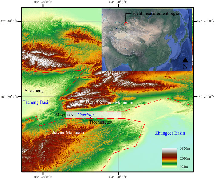
FIGURE 1. Terrain map of the Mayitas area (Sub-figure data: SIO, NOAA, U. S. Navy, NGA, GEBCO). The narrow corridor between the mountains is specially marked in Figure 1. When airflow originating from the basin moves through the narrow corridor, movement is blocked by mountains to the north and south, but the land is open to the east and west, which provides natural conditions for forming the narrow-tube effect. There are two main factors to form snowdrift: win and snow. The particular terrain of the measured area makes this area have strong wind, and both wind direction and speed are relatively stable.

This region is affected by the Siberian cold current from the west in spring and winter. On the one hand, there can occur a wide range of snowfalls in this region, and the temperature is low. It is difficult to produce freeze-thaw cycles in winter, and the state of snow particles and snow distribution, therefore, remain relatively stable. On the other hand, when airflow originating from the Tacheng Basin moves through the narrow corridor, movement is blocked by mountains to the north and south, but the land is open to the east and west. The average height difference between the narrow corridor and the mountains on both sides is above 2,100 m. The terrain provides natural conditions for forming the narrow-tube effect, which accelerates the airflow and results in strong wind flow conditions through the Mayitas region.

2.2 Drifting Snow Formation Conditions

Due to a large amount of snowfall, steady and persistent winds, and typical road sections, this area is typical for road drifting snow research. The scaled model test was conducted in this area to validate the numerical simulation accuracy in December 2019, in which weather information and the drifting snow distribution in the study area were measured. The measured location of drifting snow occurs near Tiechanggou town, with open terrain and a snow depth of 5–10 cm. The flow direction at the selected measurement site exhibits a sufficient length for snow flow development. Temperature and precipitation data were collected from the weather station at the Mayitas wind power plant, which is 20 km away from Tiechanggou town, from 11 October 2019, to 28 February 2020. The temperature and precipitation during the measurement period are shown in Figure 2. During the measurement period, the temperature ranged from −22.8°C to −1.2°C, and the average temperature reached −10.31°C. Hence, freeze-thaw cycles did not occur. Prevention of snow particle bonding on the surface of the snow layer due to freeze-thaw cycles makes it difficult for snow particles to move with the wind. A total of eight snowfall events occurred, with maximum precipitation of 5.8 mm, which provided sufficient snow sources for field measurements.

FIGURE 2

FIGURE 2. Temperature and precipitation during the measurement period. The temperature and precipitation during the measurement period are shown in Figure 2. The red dotted line shows a temperature of 0°C. The temperature during the measurement period was always below 0°C. It ensures that freeze-thaw cycles did not occur, making the snow powdery rather than sticking to each other A total of 8 snowfall events occurred, with maximum precipitation of 5.8 mm, which provided sufficient snow sources for field measurements. This satisfies another factor of the snowdrift: snow.

The ring knife method was applied to measure the accumulation density of snow particles (ρ_s) in drifting snow, and the accumulation density ranged from 0.12 to 0.3 g/m³. The projected particle size method was used to calculate the diameter of snow particles. A camera was used to collect images of snow particles in the field, and these images were transformed into grayscale images. According to a reference object (1 cm²) in the original picture, the projected area of different snow particles is calculated, and then the snow particles diameter ranged from 0.165 to 0.265 mm (Ingvander et al., 2013; Kada and Shiina, 2005). A YGY-QXY meteorological instrument was employed to automatically record the wind speed at the height of 1 m, and the measured instantaneous wind speed varied between 4.8 and 9.2 m/s.

The wind speed (at the height of 1 m) when snow particles at rest on the snow surface begin to move under the action of the wind is denoted as the starting wind speed and defined as V_t. Only then can snow particles overcome gravity and bond forces to form a snow flow. According to many observations (Kobayashi, 1972; Kane et al., 1991), the relationship between the starting wind speed V_t and the square root of the snow particle size D exhibits a linear increase (Eq. 1). The curve between V_t and snow density ρ_s is fitted considering much field-measured data (Zhu, 2007), as shown in Figure 3. This figure shows that the wind speed (4.8–9.2 m/s) at the scaled model test site meets the requirement of stable snow flow formation, which is consistent with the phenomenon observed at the site.

$\begin{array}{c}{\mathit{V}}_{\mathit{t}}=3.4+1.5\sqrt{\mathit{D}}\end{array}(1)$

FIGURE 3

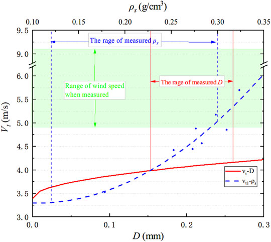
FIGURE 3. Snow particle threshold wind velocity. In Figure 3, the abscissa is the diameter of snow particles (D) and the accumulation density of snow particles (ρ_s), and the ordinate is the starting wind speed (V_t). The solid line is the relationship between D and V_t, and the dashed line is the relationship between ρ_s and V_t. The range of D and ρ_s in this measurement was marked, respectively. The green shaded area is the wind speed range when measured. The results show that the site's wind speed meets the requirement of stable snow flow formation.

2.3 Measurement Method and Model

The slope rate of the road cutting model is 2:3, the road width (W) is 20 cm, the road cutting depth (H) is 20 cm, and the projected length (B) of the slope is 30 cm. To simulate full-scale models, it is necessary to meet the geometric, kinematic, and dynamic similitude requirements (Beyers and Harms, 2003). Tabler (1980) studied the influence of scale on drifting snow tests through field measurement and found that the geometric scale model can also reflect the snow distribution law of the prototype. Due to ground roughness and wind speed limitations, the minimum scale ratio can be taken to 1/30. Also considering that the ground is not as flat as “snow-coverd lake ice,” the scale ratio of the model in this measurement is 1/25. End plates (0.4 m wide) were applied on both sides of the model to reduce end effects. The snow depth was measured via a steel drill with a length of 20 cm and a diameter of 2 mm. The layout of the steel drill is shown in Figure 4.

FIGURE 4

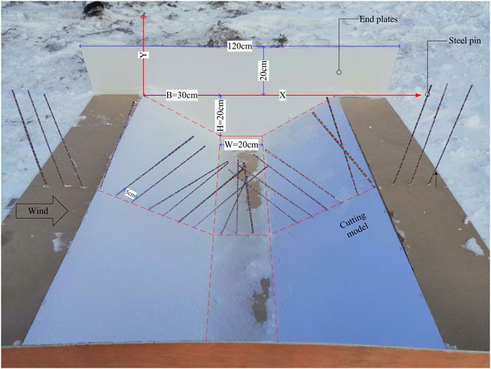
FIGURE 4. Field measurement model. Figure 4 is a photo of the cutting model in this field measurement. The coordinate axes and model dimensions are marked in the figure. Furthermore, the figure also shows the measurement method of snow depth, which is some steel drills with red, yellow, and blue labels placed on the centerline.

Before the test, a flat and open test site should be located, and a baffle should be employed in front of the test site to block snow flow at the test site during the model placement process. Shoves and pickaxes were adopted to level the site and dig a deep pit sufficient to accommodate the model. It was also necessary to ensure that no obvious fluctuations or obstacles occurred in front and at the rear of the model. Then, an anemometer was used to obtain wind field information, and the model was appropriately placed in the pit. The steel drill was inserted into the model along the central axis at intervals of 5 cm. After the test, the red and blue labels affixed on the steel drill were observed to record the snow distribution in the cutting at different times.

3 Numerical Simulation

Drifting snow flow involves multiple scales (from the snow particle scale to the topographic scale), multiple physical fields (temperature field, humidity field, wind field), and multiphase flow (snow and air) coupling (Zhou and Gu, 2006). To simplify the model, this paper adopted the Euler–Euler simulation method, added the governing equation of the snow phase to the governing equation of the air phase, and applied the mixture model to simulate multiphase flow. This approach can be employed to simulate uniform multiphase flow with solid coupling and phase movement at a constant speed, with less computation and higher computational stability, thereby allowing velocity slip of the different phases (Sun et al., 2018). Since steady-state simulation does not consider the influence of snow layer shape changes on the wind field, transient methods were implemented in this paper. In the transient method, dynamic grid technology automatically updates the near-ground grid.

3.1 Governing Equation

The mixture model considers air and snow phases and introduces the concept of the mixture phase to solve the governing equation. The continuum Eq. 2 and momentum Eq. 3 in the mixture model are as follows (Versteeg and Malalasekera, 2007):

$\begin{array}{c}\frac{\partial }{\partial \mathit{t}}\left({\mathit{\rho }}_{\mathit{m}}\right)+\nabla \cdot \left({\mathit{\rho }}_{\mathit{m}}{\mathit{v}}_{\mathit{m}}\right)=0\end{array}(2)$

$\begin{array}{c}\frac{\partial }{\partial \mathit{t}}\left({\mathit{\rho }}_{\mathit{m}}{\mathit{v}}_{\mathit{m}}\right)+\nabla \cdot \left({\mathit{\rho }}_{\mathit{m}}{\mathit{v}}_{\mathit{m}}{\mathit{v}}_{\mathit{m}}\right)=-\nabla P+\nabla \left[{\mathit{\mu }}_{\mathit{m}}\left(\nabla {\mathit{v}}_{\mathit{m}}+\nabla {\mathit{v}}_{\mathit{m}}^{\mathit{T}}\right)\right]+{\mathit{\rho }}_{\mathit{m}}g+F+\nabla \cdot \left({\displaystyle \sum }_{\mathit{k}=1}^2{\mathit{\alpha }}_{\mathit{k}}{\mathit{\rho }}_{\mathit{k}}{\mathit{v}}_{\mathit{dr},\mathit{k}}{\mathit{v}}_{\mathit{dr},\mathit{k}}\right)\end{array}(3)$

where ρ_m and v_m are the density and velocity of the mixture phase, respectively. P represents the flow field pressure, and F represents the body force; μ_m represents the hybrid viscosity of the mixture phase. v_dr,k is the relative velocity of the air and snow phases, and g is the acceleration of gravity.

The Realizable k–ε turbulence model was selected as the turbulence model, which exhibits the characteristics of a wide range and high precision among two-equation models. Compared to the Standard k–ε turbulence model, which is widely applied in engineering, the transport equation of the dissipation rate ε is modified, and the coefficient C_μ of the turbulent viscosity is no longer a constant. Yin et al. (2007) used the above turbulence model to simulate low-rise buildings, and the results indicated that the Realizable k–ε turbulence model could better simulate the fluid separation phenomenon.

The governing equation of the snow phase is expressed as Eq. 4.

$\begin{array}{c}\frac{\partial \left({\mathit{f}}_{\mathit{s}}{\mathit{\rho }}_{\mathit{s}}\right)}{\partial \mathit{t}}+\nabla \cdot \left({\mathit{f}}_{\mathit{s}}{\mathit{\rho }}_{\mathit{s}}{\mathit{v}}_{\mathit{m}}\right)=-\nabla \cdot \left({\mathit{f}}_{\mathit{s}}{\mathit{\rho }}_{\mathit{s}}{\mathit{v}}_{\mathit{dr},\mathit{s}}\right)\end{array}(4)$

where ρ_s.is the densities of the snow; f_s is the snow volume fraction. V_dr,s represents the relative slip velocity of the snow phase (Sun et al., 2018).

3.2 Erosion and Deposition of Snow

Erosion or deposition of the snow surface is determined by the friction velocity (or the wind speed) near the wall surface. When the friction velocity exceeds the threshold friction velocity of snow particles, snow particles on the wall move into the air under the action of wind and enter the computational domain, and the snow surface is eroded. When the friction velocity is lower than the threshold speed of snow particles, snow particles above the wall surface leave the computational domain and are deposited onto the wall surface. Snow erosion and deposition models (Naaim et al., 1998) are defined with Eqs 5, 6, respectively:

$\begin{array}{c}{\mathit{q}}_{\mathit{ero}}={\mathit{A}}_{\mathit{ero}}\left({\mathit{u}}_{\mathit{\ast }}^2-{\mathit{u}}_{\mathit{\ast t}}^2\right)\end{array}(5)$

$\begin{array}{c}{\mathit{q}}_{\mathit{dep}}=\varphi {\mathit{w}}_{\mathit{f}}\frac{{\mathit{u}}_{\mathit{\ast t}}^2-{\mathit{u}}_{\mathit{\ast }}^2}{{\mathit{u}}_{\mathit{\ast t}}^2}\end{array}(6)$

Eq. 7 is used to calculate the change in the snow height per unit time.

$\begin{array}{c}\mathrm{\Delta }h=\frac{{\mathit{q}}_{\mathit{ero}}+{\mathit{q}}_{\mathit{dep}}}{{\mathit{\rho }}_{\mathit{b}}}\end{array}(7)$

where A_ero is the snow erosion coefficient characterizing the cohesive force of snow, −7 × 10⁻⁴ kg-m⁻⁴-s; u* is the wall friction velocity; u_*t is the threshold wall friction velocity; w_f is the falling velocity of snow; ϕ is the near-wall snow concentration; ρ_b is the snow bulk density.

In the simulation results, the wall friction velocity u_*t is calculated via wall shear force τ₀, which is related to the velocity gradient near the wall. The calculation equation is expressed as Eq. 8.

$\begin{array}{c}{\mathit{u}}_{\mathit{\ast }}=\sqrt{\raisebox{1ex}{${\mathit{\tau }}_0$}\!\left/ \!\raisebox{-1ex}{${\mathit{\rho }}_{\mathit{a}}$}\right.}\end{array}(8)$

where ρ_a is the air density. τ₀ is the wall shear stress.

3.3 Grid and Model Parameters

Tabler (2003) verified that a geometric scaled model could also better reflect the snow distribution law of prototypes through field measurements and model experiments. Hence, the scaled model (1:25) was measured on-site. However, a full-scale model was considered in the numerical simulations in this study to reflect more details of the wind speed flow field. The cutting length is L. To ensure complete development of the flow field, the calculation range is 16L × 30H (Kang et al., 2016), and the distance from the cutting model to the entrance is 5L, as shown in Figure 5. The cutting depth is 5 m, and the cutting is of the same type (H/B and H/W) as the field-measured model.

FIGURE 5

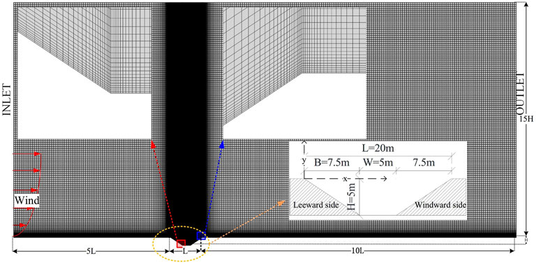
FIGURE 5. Numerical simulation model. The dimensions and grid of the numerical model are shown in Figure 5. The grid in the cutting, especially where the wind speed varies dramatically, is further refined. In addition, the defined coordinates in the cutting are shown in Figure 5.

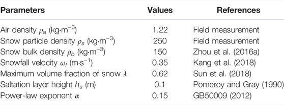
The dimensionless parameters of the prototype (scale), and full-scale CFD model are compared in Table 1. The wind velocity at 1 m in the field measurement is 4.8–9.2 m/s, and that in the CFD simulation is 4.75 m/s. H is the depth of the cutting. ν is the kinematic viscosity, which in the present study is taken as 1.79 × 10⁻⁵m²s⁻¹ (Ma et al., 2022). The measured threshold friction velocity u_*t is 0.21–0.69 m/s, and the measured Snow bulk density ρ_b is 120–300 kg/m³. The measured range of Snowfall velocity w_f is 0.2–0.5 m/s. In the numerical simulation, the diameter of snow particles is 0.2 mm, which is the average value of field measurement results. For dynamic similarity, the values of the roughness-height Reynolds number in CFD simulation is closed to field measurement. And for particles, the dimensionless similar parameters in CFD simulation are all within the range of field measurement. The field measured scale model and the numerical simulation scale model generally meet the similar conditions well.

TABLE 1

TABLE 1. Comparison of dimensionless parameters.

The height of the near-wall grid is 0.025 m, the wall friction velocity is calculated with the standard wall function, and the y + value is controlled between 30 and 300. The grid growth rate is 1.1, and the total number of grids reaches approximately 66066. The grid in the cutting, especially where the wind speed varies dramatically, is further refined. In addition, the defined coordinates in the cutting are shown in Figure 5.

3.4 Solver Settings and Boundary Conditions

The time step length was set to 0.05 s in the simulations with the moving grid technique. Changing the time step length to 0.025 and 0.075 s, it is found that the simulation results of each stage are almost the same as those of 0.05 s. The Semi-Implicit Method for Pressure-Linked Equations (SIMPLE) algorithm was adopted for pressure-velocity coupling, and the momentum equation of the second-order upwind scheme was adopted for discretization. The convergence standard required a residual smaller than 5 × 10⁻⁵.

Based on the relationship between the effective particle size of snow particles and the threshold friction velocity given by Doorschot et al. (2004), the threshold friction velocity u_*t of snow particles was calculated as 0.31 m/s under the field measurement conditions in this paper. Moreover, it should be noted that snow particles of different particle sizes can produce varied saltation lengths when snow flows move through the road cutting model. Snow particles with large particle sizes can cross the vortex region under a low wind speed by their inertia, while the vortex region mainly encompasses snow particles with small particle sizes relatively consistent with air movement due to diffusion (Kikuchi, 1981). The value of the threshold friction velocity is related to the size of snow particles. Regarding smaller snow particles, the threshold friction velocity of snow particles can decrease (Gray and Male, 1981). Therefore, in this drifting snow simulation study, the threshold friction velocity u_*t was set to 0.20 m/s.

Snow particle movement in drifting snow can be divided into creep, saltation, and suspension, of which the snow transport process caused by the latter two phenomena accounts for the majority of the movement process (Bagnold, 1941; Tominaga et al., 2011). The boundary of the snow phase entrance is controlled by the volume fraction of the snow phase in the saltation and suspension layers, as expressed in Eq. 9 (Pomeroy and Gray, 1990).

$\begin{array}{c}f\left(\mathit{x}\right)=\{\begin{array}{c}\frac{\mathit{\rho }}{3.29{\mathit{\rho }}_{\mathit{s}}{\mathit{u}}_{\mathit{\ast }}}\left(1-\frac{{\mathit{u}}_{\mathit{\ast t}}^2}{{\mathit{u}}_{\mathit{\ast }}^2}\right), \mathit{z}\le {\mathit{h}}_{\mathit{s}}\\ 0.8\mathbf{exp}\left[-1.55\left(4.78{\mathit{u}}_{\mathit{*}}^{-0.544}-{\mathit{z}}^{-0.544}\right)\right]/{\mathit{\rho }}_{\mathit{s}}, \mathit{z}>{\mathit{h}}_{\mathit{s}}\end{array}\end{array}(9)$

where f(x) represents the volume fraction of the snow phase, z represents the height above the ground. h_s is saltation layer height.

The outflow surface adopted a fully developed outflow boundary condition, symmetric boundary condition is adopted on the top of the flow region, the ground adopted a no-slip wall condition, and the wind speed at the inlet of the flow region was defined by an exponential rate wind profile, as expressed in Eq. 10.

$\begin{array}{c}U=U\left({\mathit{z}}_0\right){\left(\frac{\mathit{z}}{{\mathit{z}}_0}\right)}^{\mathit{\alpha }}\end{array}(10)$

where U(z₀) is the wind speed at the reference height (z₀ = 10 m), and 6.7 m/s is considered in this simulation study according to the field measurement results. The meanings and values of the parameters in the above equation are provided in Table 2.

TABLE 2

TABLE 2. Numerical simulation parameters.

3.5 Grid Sensitivity Test

For RANS (Reynolds-Averaged Navier-Stokes) simulation, due to the introduction of the turbulence model, when the mesh reaches a certain density, the ensemble average value does not change much, and the solution with higher precision cannot be obtained by further encryption. Grid independence verification is required. Hence, to illustrate the grid quantity of the numerical model is sufficient in this study, three different cases, that is, coarse, medium and fine, were carried out for grid independence, as shown in Table 3.

TABLE 3

TABLE 3. Specifications of grid sensitivity test.

The height of the first adjacent grid plays an important role in the boundary layer simulation. Three distinct first layer grids were used for the three testing meshes. For the high Reynolds number model (K-Epsilon model or Reynolds stress model), 30 < y⁺ < 300 is required (Ariff et al., 2009). The y⁺ of case Medium and Fine were completely in this interval, while case Coarse was not.

Figure 6A shows a comparison of the wall shear stress near the cutting under different cases. When the height of the first layer grid reaches 0.025 m, the wall shear stress will not change significantly with denser grids. Figure 6B shows the comparison of wind speeds within a height range of 70 m from the road center. Nearly no observable difference is found between the medium mesh and the fine mesh inside the cutting (0–5 m). Except for this region, the simulated wind velocity of the course case slightly differs from that of the two other cases. However, the slight difference in wind speed outside the cutting (10–50 m) has little influence on the simulation results. It appears that the medium mesh is a good compromise in terms of simulation accuracy and computational costs and, thus, the medium mesh was employed for the present study.

FIGURE 6

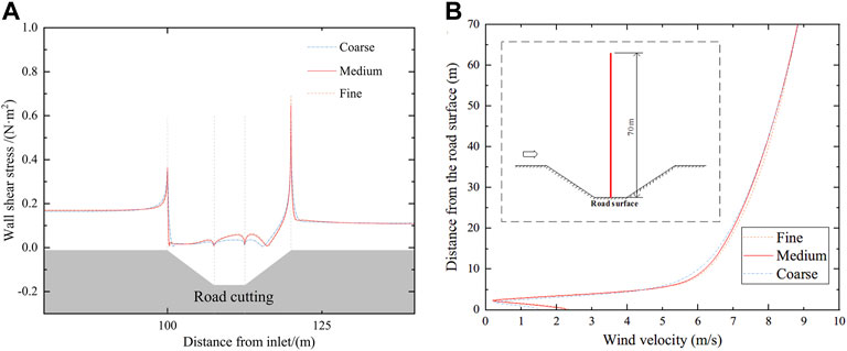
FIGURE 6. Grid sensitivity test results. To illustrate the grid quantity of the numerical model is sufficient in this study, the grid independence test was carried out. (A) comparison of the wall shear stress near the cutting under different cases. (B) comparison of wind speeds within a height range of 70 m. The results show that both accuracy and computational costs are considered in the grid in this study.

3.6 Validation

The position coordinates were dimensionless coordinates to facilitate comparison between the field measurements and numerical simulation results, defined as x′ = x/L and y′ = y/H. As such, the wind blowing time was also dimensionless. The Anno (1984) method was applied at the processing step. The corresponding relationship between the measured and simulated times is expressed as Eq. 11.

$\begin{array}{c}\frac{{\mathit{t}}_{\mathit{f}}}{{\mathit{Q}}_{\mathit{sal}\_\mathit{s}}}=\frac{{\mathit{t}}_{\mathit{s}}}{{\mathit{Q}}_{\mathit{sal}\_\mathit{f}}}\end{array}(11)$

where t_f and t_s denote the measurement and simulation times, respectively, Q_{sal_f} and Q_{sal_s} denote the measured and simulated snow transport rates, respectively, which can be calculated with Eq. 12, namely, Q_{sal_f} = 0.3 × 10⁻³ kg/m-s and Q_{sal_s} = 7.4 × 10⁻³ kg/m-s.

$\begin{array}{c}\mathit{Q}=\frac{0.68\mathit{\rho }{\mathit{u}}_{\mathit{\ast t}}}{\mathit{g}{\mathit{u}}_{\mathit{\ast }}}\left({\mathit{u}}_{\mathit{\ast }}^2-{\mathit{u}}_{\mathit{\ast t}}^2\right)\end{array}(12)$

Adopting the snow height at the center of the road cutting as a reference, it was found that the snow height at the end of the measurement time (t_f = 2,280 s) equaled that at the end of the simulation time (t_s = 28,100 s). On this basis, the time was made dimensionless in combination with Eq. 11, as defined in Eq. 13 and listed in Table 4.

$\begin{array}{c}{\mathit{t}}^{\mathit{\ast }}=\frac{{\mathit{t}}_{\mathit{f}}{\mathit{Q}}_{\mathit{sal}\_\mathit{f}}}{{\mathit{\rho }}_{\mathit{s}}{\mathit{H}}^2}\end{array}(13)$

where H is the cutting depth.

TABLE 4

TABLE 4. Time correspondence between the measurement and the simulation times.

The snow layer evolution process corresponding to the field measurements and numerical simulation results at different times is shown in Figure 7.

FIGURE 7

FIGURE 7. Validation of the snow cover evolution process. Curves of the same color in Figure 6 are respectively the snow distribution results of field measurement and numerical simulation at the same moment. Furthermore, the curve with hollow labels is the result of numerical simulation. During each phase, the simulated snow volume was consistent with the measured snow volume, which reveals that the snow accumulation process in the road cutting is consistent between the field measurements and numerical simulation results.

Figure 7 reveals that the snow accumulation process in the road cutting is basically consistent between the field measurements and numerical simulation results. Snow was first generated on the leeward-side slope, and due to the considerable amount of snow, the front edge of the leeward-side slope generated snow sedimentary bodies. Then, snow began to accumulate on the windward side of the slope but only within half of the slope near the foot. The increase in the snow on both sides resulted in slope steepening, after which snow accumulation on the road began to increase rapidly.

It should be noted that the snow cover appears to differ between the analysis and experiment for x’<0.5. The main difference is that the location of the cornice is closer to the top of the leeward slope in the field measurement. The location of the cornice is related to the vortex (separation point) in the cutting. Furthermore, the snow supplement, wind speed and direction change with time in the field measurement but are set as constant in the numerical simulation. This leads to a more stable vortex in numerical simulations.

The result of the stable vortex is that more snow particles are deposited around the vortex separation point. The same effect is produced at the vortex attachment point as proof. In addition, the erosion and deposition model selected for the simulation did not consider the weight of the snow and the repose angle. These reasons together lead to the differences between the analysis and experiment in snow cover on both sides of the slope.

However, relative to both sides of the slope, the snow cover on the road surface has a better coincidence. The snow cover evolution process in each stage is basically the same, proving that using this numerical simulation method and the corresponding parameters to simulate snowdrift on road cutting is feasible.

4 Numerical Simulation Results

To reveal the formation mechanism of drifting snow disasters in road cuttings, the wind speed flow field, wall friction velocity, and snow evolution process at different stages were analyzed in detail based on the simulation results.

4.1 Flow Field

The deposition or erosion of snow particles at a particular location is strongly related to the wind speed flow field. Therefore, this section first analyzes the wind flow field around the cutting at different times. Four cutting flow fields at representative times (t* = 0, 0.02, 0.07, and 0.14) are selected, and the wind streamlines around the cutting are shown in Figure 8.

FIGURE 8

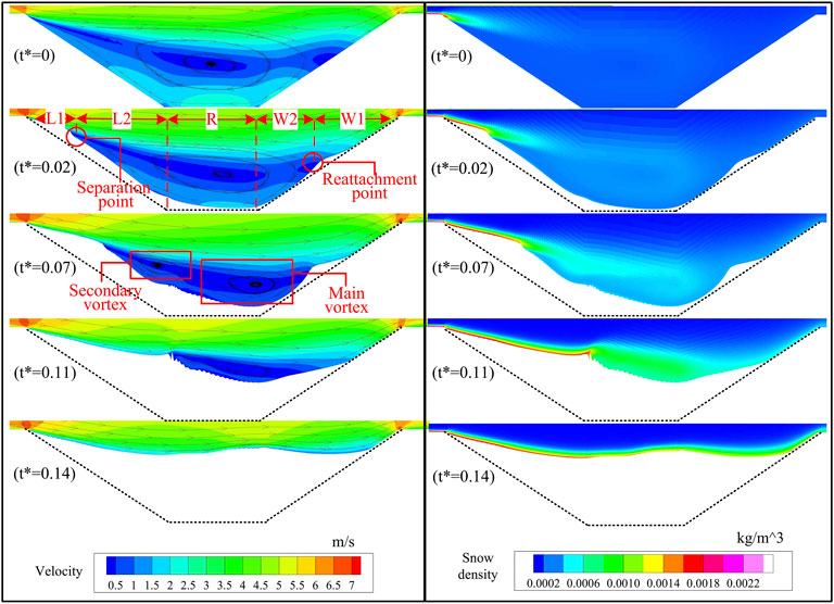
FIGURE 8. Flow field and snow density around the road cutting at different times. Cutting flow fields and wind streamlines around the cutting at representative times are shown in Figure 7. The vortex separation point and reattachment point are marked in the figure, which divides the road cutting into five areas. In Figure 7, the position of the secondary vortex is also specially marked. Its appearance divides the road cutting wind blowing snow disaster into three stages. The variation of two points and vortex scale in each stage is described.

At the initial moment (t* = 0), the flow separated at the top of the leeward side, forming a large-scale vortex within the cutting, which could reduce the wind speed and wall friction velocity inside the cutting, resulting in the accumulation of snow particles. On the windward-side slope, flow reattachment occurred. There was a good correspondence between the distribution of the low-wind speed area and vortex. The wind speed at the vortex center was the lowest. With increasing distance from the vortex center, the wind speed gradually increased.

With increasing snow accumulation in the cutting caused by drifting snow (t* = 0.02), the vortex separation point continuously moved toward the center of the cutting, but the position of the vortex reattachment point remained almost unchanged, always approximately 1/2 of the windward-side slope. Moreover, the size of the vortices in the cutting decreased, and the size of the low-wind speed area decreased, as shown in Figure 9. Through observation, it is found that the location of snow accumulation is strongly correlated with the area with wind speed of 1 m/s. Therefore, for statistical convenience, the area with wind speed of less than 1 m/s is defined as the low-wind area. However, due to the influence of the snow cover, the whole road cutting section also decreased, and the proportion of the low-wind area overall increased.

FIGURE 9

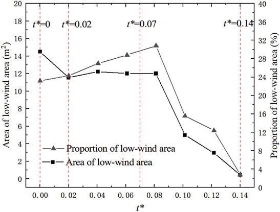
FIGURE 9. Low-wind area around the cutting. The formation of drifting snow disasters is correlated with low-wind speed areas. It is observed from the simulation results that the location of the snow cover is related to the area where the wind speed is less than 1 m/s. Therefore, changes in the low-wind speed area within the whole cutting range are analyzed, as shown in Figure 8. Before the secondary vortex disappears, the proportion of low-wind speed area increases.

With increasing snow cover (t* = 0.07), when the vortex separation point advanced to approximately 1/2 of the leeward-side slope, the height of the vortex reattachment point rose, and a secondary vortex was formed in the cutting. The emergence of the secondary vortex directly divided the scale of the main vortex, which resulted in the low-wind area almost filling the whole road cutting. At t* = 0.14, the cutting was almost entirely submerged by snow, the vortex disappeared, and flow separation and reattachment no longer occurred.

The maximum value of the snow density at the top of the leeward slope at different times is the snow phase concentration at the saltation layer of the incoming flow. Furthermore, with the increase of snow drifting time, the concentration of snow phase in the middle of the cutting increases. The snow particles diffused from the cutting center to slopes and road surface, and the concentration gradually decreased.

According to the location of the vortex separation and reattachment points, the cutting was partitioned, and the partition results are shown in Figure 7. The leeward- and windward-side slopes of the cutting are denoted as L and W, respectively, and the road surface is denoted as R. Due to the great difference between the vortex separation point and the friction velocity on both sides of the vortex reattachment point, in L, the range from the top of the leeward-side slope to the point of the vortex separation point is L1, and the other range of L is denoted as L2. In W, the range from the top of the windward-side slope to the vortex reattachment point of the windward slope is W1, and the other range is denoted as W2. It is important to note that L1, L2, W1, and W2 are in time-varying ranges, while R remain fixed. This is due to the changes of vortex separation point and vortex reattachment point in the simulation process. According to the emergence and disappearance times of the secondary vortex, drifting snow disasters in road cuttings can be divided into three stages. Stage 1 extends from the initial time to the formation of the secondary vortex (t* = 0.07), and stage 2 extends from the formation of the secondary vortex to its disappearance (t* = 0.11). After that, until the main vortex disappears, stage 3 (t* = 0.14) applies. After the disappearance of the main vortex, the road cutting is completely submerged, and the snow distribution in the road cutting remains stable and no longer changes.

4.2 Wall Friction Velocity

The wall friction velocity u_* is another critical parameter most related to the position of snow accumulation or erosion. The wind speed flow field mainly reflects the wind speed in the cutting, while the friction velocity near the wall represents the wind speed on the ground. According to the characteristics of the snow erosion model, the wall friction velocity is dimensionless. The snow variation coefficient C_u* is defined in Eq. 14. If C_u* is positive, snow is eroded. Conversely, snow deposition occurs. The higher the value is, the higher the erosion or deposition rate. Figure 10 shows the snow variation coefficient C_u* at the different stages in each cutting area.

$\begin{array}{c}{\mathit{C}}_{\mathit{u\ast }}=\raisebox{1ex}{$\left({\mathit{u}}_{\mathit{\ast }}-{\mathit{u}}_{\mathit{\ast t}}\right)$}\!\left/ \!\raisebox{-1ex}{${\mathit{u}}_{\mathit{\ast t}}$}\right.\end{array}(14)$

FIGURE 10

FIGURE 10. Wall friction velocity at the different stages. Due to the snow erosion deposition model used in this study, The wall friction velocity u* is another critical parameter that is most related to the position of snow accumulation or erosion. The wind speed flow field mainly reflects the wind speed in the cutting, while the friction velocity near the wall represents the wind speed on the ground. In Figure 9, the changes of u* in each stage are described in detail, which is dimensionless defined as C_u*.

At stage 1, the wall friction velocity changed little over the whole cutting range. In the beginning, the whole leeward slope comprised a snow deposit area. With the deposition of snow particles at the top of the leeward slope, the proportion of the L1 region, which is constantly eroded, gradually increased. It should be noted that L1 and L2, as marked in Figure 9, represent moments at the end of stage 1. The road surface also constituted a snow particle deposition area. From the windward side to the leeward side of the slope foot, the snow rate gradually increased. In the W2 region, there occurred apparent snow deposition at the vortex reattachment point, and the W1 region comprised a snow erosion region.

After the emergence of the secondary vortex (stage 2), the friction velocity near the wall significantly changed over the whole cutting range. The proportion of L1 increased rapidly, and by the end of stage 2, the entire leeward side of the cutting comprised a stable L1 area. The snow deposition rate in the road surface area increased, and the gain effect was more apparent closer to the windward slope foot, which resulted in a moderate snow deposition rate in the road surface area. After the emergence of the secondary vortex, the deposition rate of snow particles in the W2 region rapidly increased, while that in the W1 region remained stable.

After the disappearance of the secondary vortex, the drifting snow disaster reached stage 3. The wall friction velocity remained highly consistent on the leeward slope, and the whole leeward slope occurred within the range of snow erosion. The change in friction velocity at the road surface remained obvious, but the range of snow deposition contracted. With increasing snow height, the snow cover on the windward side moved from the vortex reattachment point to the top of the windward-side slope. To analyze the snow cover rate in the various areas at the different stages more detailedly, the average snow cover variation coefficient (wall friction velocity) in each region at each moment was calculated, as shown in Figure 11.

FIGURE 11

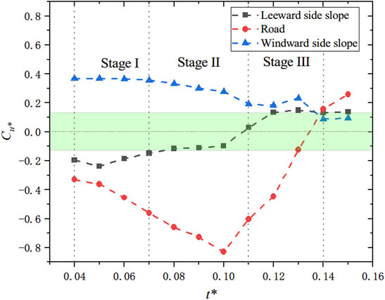
FIGURE 11. Snow variation coefficient at the different stages. The variation of u* on both sides of slope and road surface is analyzed as shown in Figure 10. The snow deposition rate can be analyzed from the figure, which has different characteristics on road surface and slope. The windward-side slope is the most stable and has been in a state of snow erosion. In the beginning, the leeward side slope was in a state of snow deposition. After the emergence of the secondary vortex, it also entered a relatively stable state. The change of road surface is the most dramatic, and the snow deposition rate increases almost all the time before the disappearance of the main vortex.

The smaller the absolute value of C_u*, the smaller the change of snow height is, indicating that the erosion and deposition of snow have reached a balance. As shown in Figure 10, the leeward-side slope existed in a state of snow particle deposition before the disappearance of the secondary vortex and after that in a state of erosion. The main changes in the road snow cover occurred at stages 2 and 3. The snow deposition rate in the road cutting at stage 2 increased gradually and reached its highest value at t* = 0.10. At stage 3, the road snow cover rate rapidly declined, and the snow cover in the road cutting was eroded in the end. As approximately 1/3 of the area on the windward-side slope always exhibited a lack of snow deposition, the windward-side slope manifested snow erosion overall. However, the erosion rate gradually decreased. It is reasonable to speculate that the snow deposition rate in the W2 region increased at stages 1, 2, and 3.

4.3 Snow Evolution Process

In the process of increasing the snow volume, the first segment to be observed is the leeward-side slope top, where the speed of drifting snow flow decreased by 80% upon entering the cutting. This segment became the first area with a low-wind speed along the direction of storm flow, resulting in the accumulation of many snow particles, forming a characteristic snow cornice, as shown in Figure 12. The cornice face advanced along the slope with increasing snow particle accumulation, and the cornice roof grew in length. It should be noted that the roof was balanced between erosion and deposition, with a gradient of 1:4. At this time, snow accumulation on the windward side of the slope was mainly generated near the vortex reattachment point at the center of the slope, and snow on the road was mainly accumulated on the leeward side of the slope foot.

FIGURE 12

FIGURE 12. Simulated snow distribution. In Figure 11, the results of the snow evolution process in road cutting are presented. Snow cornice is formed on the leeward side slope. Its face and roof have certain characteristics. The cornice roof remained balanced between erosion and deposition, creating a new leeward-side slope with a slope ratio of 1:4. Moreover, the position of its face is related to the formation of the secondary vortex.

When the cornice face advanced 1/2 of the leeward-side slope, a secondary vortex formed in region L2. After the emergence of the secondary vortex, the snow height in region L2 increased rapidly. Uplift of the snow surface in region L2 greatly influenced the flow field in zones R and W2. The increase in snow cover height in region W2 was particularly obvious, and the snowpack volume in this region was almost zero before the emergence of the secondary vortex. Snow on the slopes on both sides of the road surface increased simultaneously, advancing toward the cutting center. Then, the main vortex scale decreased, and the proportion of the low-wind area in the vortex increased, which is the main reason for the observed snow disaster in the road cutting.

After the cornice face advanced toward the leeward slope foot, the secondary vortex disappeared, and the snow cover in region L1 remained stable and almost no longer increased. The increase in snow cover in region W2 also significantly declined. The snow cover in region R was affected by the still present main vortex, and the snow cover continued to increase. When the snow surface in all regions remained stable, the main vortex also disappeared, the snow layer remained stable and mostly did not change, and the road cutting was entirely submerged by snow.

To quantify the concerned road snow cover rate and amount, the road section area (25 m²) at the initial moment was considered to determine the dimensionless snow volume, and the changes at the different stages are shown in Figure 13.

FIGURE 13

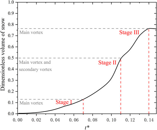
FIGURE 13. Snow volume on the road at the different stages. To quantify the concerned road snow cover rate and amount, the changes of snow volume at the different stages are shown in Figure 12. Before the cornice advanced toward the center of the leeward-side slope, this period of the main vortex acting alone constituted the drifting snow safety period of the cutting. The period from the appearance of the secondary vortex to the disappearance of the secondary vortex represented the period with a rapid increase in the snow cover. After the secondary vortex disappeared, the snow deposition rate slowed down.

Figure 12 shows that the rapid growth period of the road snow cover started when the secondary vortex appeared and ended after the disappearance of the main vortex. It could be considered that before the emergence of the secondary vortex, i.e., before the cornice advanced toward the center of the leeward-side slope, this period of the main vortex acting alone constituted the drifting snow safety period of the cutting. The period from the appearance of the secondary vortex to the disappearance of the secondary vortex represented the period with a rapid increase in the snow cover.

Particular attention should be given when a cornice is present on the leeward side of the slope. Its appearance greatly influences the rear flow field, which is the primary reason for a series of problems, such as the appearance of secondary vortices and the arrival of the rapid growth period of snow. Furthermore, by observing the snow distribution in the road cutting, it was found that the drifting snow safety stage of the road cutting included a safe storage period in terms of time and a safe storage area in terms of location.

Under a steep cutting slope and emergence of the secondary vortex (t* = 0.07), there could be cornice present on the leeward side of the slope. The trapezoid obtained by extending the cornice along the slope direction was defined as the snow storage area. When the amount of snow on the slope increases, and before the emergence of the secondary vortex, the cornice slope reached 1:4, and the top surface of the trapezoidal always remained parallel to the slope. Therefore, the stable area was defined as the critical snow storage area of the cutting, as shown in Figure 14, which could be adopted as an index to measure the snow storage capacity of the cutting.

FIGURE 14

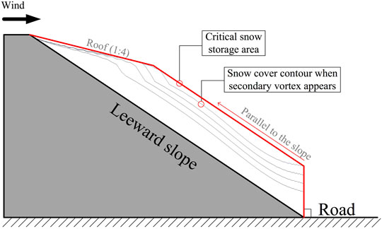
FIGURE 14. Critical snow storage area. The trapezoid obtained by extending the cornice along the slope direction was defined as the snow storage area, which is defined as the snow storage area. Furthermore, it could be adopted as an index to measure the snow storage capacity of the cutting. The road surface can be cleared if the snow amount on the leeward side of the cutting is smaller than the critical amount of snow storage in the event of a snow disaster. And the road cutting does not enter the stage of rapid snow accumulation.

The road surface can be cleared if the snow amount on the leeward side of the cutting is smaller than the critical amount of snow storage in a snow disaster. Otherwise, the cutting can reach the stage of rapid snow increase, resulting in road submergence. When the slope cannot be changed, appropriately lengthening the cutting, i.e., deepening the cutting depth, could enhance the critical snow storage capacity.

5 Conclusion

The mixture model and the transient method were adopted to simulate snow redistribution in road cuttings. The simulation results suitably agreed with the field-measured results. In practice, the factors that affect the evolution of road cutting snow may be affected by other factors, such as wind speed, wind direction, the depth and slope of the cutting, and the height difference between two sides of the slope top. This study only investigated the influence of the inclination of the wind deflectors and simulated them under ideal conditions, such as constant wind speed, wind direction, and sufficient snow supplementation. Our results and calculations provide a preliminary reference for future investigations. This study is a typical case in many working conditions. Through further analysis of the flow field, snow evolution process, and wall friction velocity, the formation mechanism and controlling measure of drifting snow disasters in road cuttings was summarized, which provides a preliminary reference for future investigations. The main conclusions are as follows:

1) When drifting snow flow moved through the cutting, there occurred vortex of a certain scale in the cutting, and the range of these vortices was consistent with the position of snow particle accumulation. Vortex separation and reattachment points were observed on the slopes on both sides of the vortex, and snow deposition always occurred between these two points. The vortex separation point continuously advanced toward the cutting center along the slope direction with increasing snow cover. The position of the vortex reattachment point only increased along the height direction but hardly varied along the horizontal direction.

2) The appearance of a secondary vortex constituted a critical indication of the rapid growth stage of the snow cover. The appearance and disappearance of secondary vortex could be divided into three stages of snow cover evolution. Stage 1 is the safe storage period, and stage 2 is the rapid growth period. The size of the low-wind speed area was positively correlated with the vortex scale, and the proportion of the low-wind speed area increased during the safe storage and rapid growth periods. The key to preventing and controlling drifting snow disasters is to treat snow promptly before the rapid growth period.

3) In the process of snow accumulation from the initial state in the cutting, a stable cornice emerged at the top of the leeward-side slope. The cornice roof remained balanced between erosion and deposition, creating a new leeward-side slope with a slope ratio of 1:4. The cornice face advanced toward the cutting center along the leeward-side slope with an angle ranging from 55° to 60°.

4) A secondary vortex occurred in the cutting as the snow cornice advanced across 1/2 of the leeward-side slope. Before the emergence of the secondary vortex, the increase in the snow on the road surface occurred slowly, and there existed a critical snow storage area on the leeward-side slope, which could accommodate a considerable snow amount. When the predicted amount of incoming snow is smaller than the critical amount of snow storage, the road cutting does not enter the stage of rapid snow accumulation.

Data Availability Statement

The raw data supporting the conclusion of this article will be made available by the authors, without undue reservation.

Author Contributions

WM: Supervision, Methodology, Writing—review, and editing; SL: Writing—original draft preparation, Investigation, and Visualization; YS: Funding acquisition and Supervision; JL: Software; FL: Validation.

Conflict of Interest

Authors YS was employed by China Railway Design Corporation.

The remaining authors declare that the research was conducted in the absence of any commercial or financial relationships that could be construed as a potential conflict of interest.

Publisher’s Note

All claims expressed in this article are solely those of the authors and do not necessarily represent those of their affiliated organizations, or those of the publisher, the editors and the reviewers. Any product that may be evaluated in this article, or claim that may be made by its manufacturer, is not guaranteed or endorsed by the publisher.

Acknowledgments

The authors gratefully acknowledge the support of the Education Department of Hebei Province (Grant No. ZD2018063).

References

Adok, U. (1977). Snow Drift. J. Glaciol. 19 (81), 123–139. doi:10.3189/S0022143000215591

CrossRef Full Text | Google Scholar

Anno, Y. (1984). Requirements for Modeling of a Snowdrift. Cold regions Sci. Technol. 8 (3), 241–252. doi:10.1016/0165-232X(84)90055-7

CrossRef Full Text | Google Scholar

Ariff, M., Salim, S. M., and Cheah, S. C. (2009). “Wall Y+ Approach for Dealing with Turbulent Flow over a Surface Mounted Cube: Part 2–high Reynolds Number,” in Seventh International Conference on CFD in the Minerals and Process Industries CSIRO (CSIRO Publishing: Melbourne, Australia), 9.

Google Scholar

Bagnold, R. A. (1971). The Physics of Blown Sand and Desert Dunes Methuen London. London: Methuen & Co, 265. doi:10.1007/978-94-009-5682-7

CrossRef Full Text | Google Scholar

Beyers, J. H. M., and Harms, T. M. (2003). Outdoors Modelling of Snowdrift at SANAE IV Research Station, Antarctica. J. Wind Eng. Industrial Aerodynamics 91 (4), 551–569. doi:10.1016/S0167-6105(02)00409-9

CrossRef Full Text | Google Scholar

GB50009 (2012). Load Code for the Design of Building Structures. Beijing: China Architecture and Building Press.

Google Scholar

Gray, D. M., and Male, D. H. (1981). Handbook of Snow: Principles, Processes. Management and Use. Toronto: The Blackburn Press.

Google Scholar

Hawley, R. L., and Millstein, J. D. (2019). Quantifying Snow Drift on Arctic Structures: A Case Study at Summit, Greenland, Using UAV-Based Structure-From-Motion Photogrammetry. Cold Regions Sci. Technol. 157, 163–170. doi:10.1016/j.coldregions.2018.10.007

CrossRef Full Text | Google Scholar

Ingvander, S., Brown, I. A., Jansson, P., Holmlund, P., Johansson, C., and Rosqvist, G. (2013). Particle Size Sampling and Object-Oriented Image Analysis for Field Investigations of Snow Particle Size, Shape, and Distribution. Arct. Antarct. Alp. Res. 45 (3), 330–341. doi:10.1657/1938-4246-45.3.330

CrossRef Full Text | Google Scholar

JDoorschot, J. J., Lehning, M., and Vrouwe, A. (2004). Field Measurements of Snow-Drift Threshold and Mass Fluxes, and Related Model Simulations. Boundary-Layer Meteorol. 113 (3), 347–368. doi:10.1007/s10546-004-8659-z

CrossRef Full Text | Google Scholar

Kada, W., and Shiina, T. (2005). “Snow Particle Extraction and Analysis Using the Differential of Sequential Images,” in Proceedings. 2005 IEEE International Geoscience and Remote Sensing Symposium (New York: IEEE), 6, 3986–3989. IGARSS'05. doi:10.1109/IGARSS.2005.1525787

CrossRef Full Text | Google Scholar

Kane, D. L., Hinzman, L. D., and Zarling, J. P. (1991). Thermal Response of the Active Layer to Climatic Warming in a Permafrost Environment. Cold Regions Sci. Technol. 19 (2), 111–122. doi:10.1016/0165-232X(91)90002-X

CrossRef Full Text | Google Scholar

Kang, L., Zhou, X., and Gu, M. (2016). Numerical Simulation Method about Snowdrift on Roofs with Consideration of Repose Angle of Snow. J. Tongji Univ. 44 (1), 11–15. doi:10.11908/j.issn.0253-374x.2016.01.002

CrossRef Full Text | Google Scholar

Kang, L., Zhou, X., van Hooff, T., Blocken, B., and Gu, M. (2018). CFD Simulation of Snow Transport over Flat, Uniformly Rough, Open Terrain: Impact of Physical and Computational Parameters. J. Wind Eng. Industrial Aerodynamics 177, 213–226. doi:10.1016/j.jweia.2018.04.014

CrossRef Full Text | Google Scholar

Kikuchi, T. (1981). A Wind Tunnel Study of the Aerodynamic Roughness Associated with Drifting Snow. Cold Regions Sci. Technol. 5 (2), 107–118. doi:10.1016/0165-232X(81)90045-8

CrossRef Full Text | Google Scholar

Kobayashi, D. (1972). Studies of Snow Transport in Low-Level Drifting Snow. Contributions Inst. Low Temp. Sci. 24, 1–58.

Google Scholar

Liu, M., Zhang, Q., Fan, F., and Shen, S. (2018). Experiments on Natural Snow Distribution Around Simplified Building Models Based on Open Air Snow-Wind Combined Experimental Facility. J. Wind Eng. Industrial Aerodynamics 173, 1–13. doi:10.1016/j.jweia.2017.12.010

CrossRef Full Text | Google Scholar

Liu, Z., Yu, Z., Zhu, F., Chen, X., and Zhou, Y. (2019). An Investigation of Snow Drifting on Flat Roofs: Wind Tunnel Tests and Numerical Simulations. Cold regions Sci. Technol. 162, 74–87. doi:10.1016/j.coldregions.2019.03.016

CrossRef Full Text | Google Scholar

Ma, W., Luo, Y., Li, F., and Sun, Y. (2022). The Influence of Wind Deflectors on the Snow Distribution in Road Cuttings during Snowdrift. Cold Regions Sci. Technol. 196, 103505.

CrossRef Full Text | Google Scholar

Naaim, M., Naaim-Bouvet, F., and Martinez, H. (1998). Numerical Simulation of Drifting Snow: Erosion and Deposition Models. A. Glaciol. 26, 191–196. doi:10.3189/1998AoG26-1-191-19610.1017/s0260305500014798

CrossRef Full Text | Google Scholar

Oikawa, S., Tomabechi, T., and Ishihara, T. (1999). One-day Observations of Snowdrifts Around a Model Cube. J. Snow Eng. Jpn. 15 (4), 283–291. doi:10.4106/jsse.15.4_283

CrossRef Full Text | Google Scholar

Okaze, T., Mochida, A., Tominaga, Y., Nemoto, M., Sato, T., Sasaki, Y., et al. (2012). Wind Tunnel Investigation of Drifting Snow Development in a Boundary Layer. J. wind Eng. industrial aerodynamics 104-106, 532–539. doi:10.1016/j.jweia.2012.04.002

CrossRef Full Text | Google Scholar

Pomeroy, J. W., and Gray, D. M. (1990). Saltation of Snow. Water Resour. Res. 26 (7), 1583–1594. doi:10.1029/WR026i007p01583

CrossRef Full Text | Google Scholar

Sun, X., He, R., and Wu, Y. (2018). Numerical Simulation of Snowdrift on a Membrane Roof and the Mechanical Performance under Snow Loads. Cold Regions Sci. Technol. 150, 15–24. doi:10.1016/j.coldregions.2017.09.007

CrossRef Full Text | Google Scholar

Tabler, R. D. (2003). Controlling Blowing and Drifting Snow with Snow Fences and Road Design. Washington, DC: Transportation Research Board. (No. NCHRP Project 20-7 (147)).

Google Scholar

Tabler, R. D. (1980). Self-similarity of Wind Profiles in Blowing Snow Allows Outdoor Modeling. J. Glaciol. 26 (94), 421–434. doi:10.3189/S0022143000010947

CrossRef Full Text | Google Scholar

Thiis, T. K., and Gjessing, Y. (1999). Large-scale Measurements of Snowdrifts Around Flat-Roofed and Single-Pitch-Roofed Buildings. Cold regions Sci. Technol. 30 (1-3), 175–181. doi:10.1016/s0165-232x(99)00021-x

CrossRef Full Text | Google Scholar

Tominaga, Y., Okaze, T., and Mochida, A. (2011). CFD Modeling of Snowdrift Around a Building: An Overview of Models and Evaluation of a New Approach. Build. Environ. 46 (4), 899–910. doi:10.1016/j.buildenv.2010.10.020

CrossRef Full Text | Google Scholar

Tominaga, Y., Shirzadi, M., Inoue, S.-i., Wakui, T., and Machida, T. (2020). Computational Fluid Dynamics Simulations of Snow Accumulation on Infrared Detection Sensors Using Discrete Phase Model. Cold Regions Sci. Technol. 180, 103167. doi:10.1016/j.coldregions.2020.103167

CrossRef Full Text | Google Scholar

Tsuchiya, M., Tomabechi, T., Hongo, T., and Ueda, H. (2002). Wind Effects on Snowdrift on Stepped Flat Roofs. J. wind Eng. industrial aerodynamics 90 (12-15), 1881–1892. doi:10.1016/S0167-6105(02)00295-7

CrossRef Full Text | Google Scholar

Versteeg, H. K., and Malalasekera, W. (2007). An Introduction to Computational Fluid Dynamics: The Finite Volume Method. New York: Pearson education.

Google Scholar

Wang, J., Liu, H., Chen, Z., and Ma, K. (2020). Wind Tunnel Test of Wind-Induced Snowdrift on Stepped Flat Roofs during Snowfall. Nat. Hazards 104 (1), 731–752. doi:10.1007/s11069-020-04188-1

CrossRef Full Text | Google Scholar

Yin, H., Zhang, Q., and Zhou, Z. (2007). Numerical Simulation Study of 3D Steady Atmospheric Flow Around Standard Low-Rise Building TTU Model. Eng. Mech. 24 (2), 0–145.

Google Scholar

Zhang, G., Zhang, Q., Fan, F., and Shen, S. (2021). Numerical Simulations of Development of Snowdrifts on Long-Span Spherical Roofs. Cold Regions Sci. Technol. 182, 103211. doi:10.1016/j.coldregions.2020.103211

CrossRef Full Text | Google Scholar

Zhou, X., and Gu, M. (2006). “Numerical Simulation of Snow Drift on the Surface of a Large-Span Roof Structure,” in proceedings of Fourth International Symposium on Computational Wind Engineering (CWE2006), Yokohama, Japan, July 16-19, 2006, 889–892.

Google Scholar

Zhou, X., Kang, L., Gu, M., Qiu, L., and Hu, J. (2016a). Numerical Simulation and Wind Tunnel Test for Redistribution of Snow on a Flat Roof. J. Wind Eng. Industrial Aerodynamics 153, 92–105. doi:10.1016/j.jweia.2016.03.008

CrossRef Full Text | Google Scholar

Zhou, X., Qiang, S., Peng, Y., and Gu, M. (2016b). Wind Tunnel Test on Responses of a Lightweight Roof Structure under Joint Action of Wind and Snow Loads. Cold Regions Sci. Technol. 132, 19–32. doi:10.1016/j.coldregions.2016.09.011

CrossRef Full Text | Google Scholar

Zhu, G. (2007). Formation Mechanism and Prevention of Drifting Snow Disasters on Highway. Harbin, China: Heilongjiang People’s Publishing House. (In Chinese).