Multi-Scale Normalization Method Combined With a Deep CNN Diagnosis Model of Dynamometer Card in SRP Well

There are more than 20 types of dynamometer card measured of sucker rod pumping (SRP) wells in oil fields, and some working conditions are very complicated. The common diagnosis model of SRP well based on dynamometer card recognition has low accuracy and recall rate of complicated working conditions. In order to improve the accuracy and recall rate of multi-condition diagnosis of SRP well and solve the problem of inseparable data attributes caused by traditional dynamometer card normalization methods, a new dynamometer card preprocessing method is proposed, which uses a clustering analysis algorithm to obtain multiple normalized dynamometer cards of the original dynamometer card and at the same time, adds a set of time-series dynamometer cards to enhance the separability of data. The dynamometer card preprocessing method combined with four deep convolutional neural networks are used to build a diagnosis model. Experiments are conducted under 24 different working conditions, the accuracy of our method is up to 95.8%, and the average recall rate of complicated working conditions is up to 93.1%, which is 13.6 and 35.3% higher than that of the model (AlexNet) built by the traditional preprocessing method. In addition, the preprocessing method of dynamometer card proposed is applicable to all deep learning models and machine learning models. Field applications show that our method is very effective for recalling abnormal working conditions, which is of great significance to the real demand for intelligent diagnosis of SRP well.

Introduction

The sucker rod pumping (SRP) is the main artificial lifting method for oil wells. Because the rods, pipes, and pumps of SRP work in a harsh environment, the SRP wells frequently fail after long-term operation. Real-time diagnosis of downhole working conditions and finding the causes of production changes in abnormal working conditions can help avoid further deterioration. The dynamometer card is a closed curve diagram composed of the relationship between load and displacement. The dynamometer card showing the relationship between the polished rod load and the displacement is called the surface dynamometer card. Generally, the surface dynamometer card is used as the main basis for analyzing the working conditions of the SRP well (Eickmeier 1967) because it can reflect the downhole working condition, which includes a pump, sucker rod, and wellbore. With the development of artificial intelligence technology and the petroleum industry’s emphasis on digitization and intelligence, technologies such as machine learning and deep learning-based working condition diagnosis and early warning of SRP well have been applied and developed. There are two different types of diagnosis models based on dynamometer card classification. The first is the tow-step model, which includes dynamometer card feature extraction and pattern classification. Many dynamometer card feature extraction methods are used, such as centroid, curvature descriptor, Fourier descriptor and geometric moment vector (de Lima et al., 2012), and Freeman chain code (Li et al., 2013a); Fourier descriptor has good calculation speed and feature description ability (Yu et al., 2013). Pattern classification methods include support vector machines (SVMs; Li et al., 2013b), gradient-boosted decision tree (GBDT; Bangert et al., 2019), and artificial neural network (ANN; Xu et al., 2007; Bezerra et al., 2009; Abdalla et al., 2020). However, this kind of method is less effective in multi-condition diagnosis tasks because the feature extraction method itself will lose more information. The second model uses a convolutional neural network to complete feature extraction and classification in one step without human effort and prior knowledge. Boguslawski et al. (2018) used a variety of deep learning fusion models in edge computing to realize the diagnosis of eight downhole conditions, combining the advantages of all models to get the best result; Wang et al. (2021) used two-time overlay dynamometer card as the CNN input to enhance the data classification features. However, there are actually a variety of working conditions in the oil field, which are complicated and diverse, and the dynamometer card types can reach more than 20 types. There are a large number of complicated dynamometer cards other than typical dynamometer cards; it is difficult to identify the dynamometer cards of these complicated working conditions with those models. Although the complicated working conditions occur in a small number of oil wells, they seriously affect the production of the oil wells. Wrong diagnosis of a small number of wells with complicated working conditions as normal production wells will not significantly affect the accuracy rate of the model, only reduce the recall rate of the corresponding working conditions. Therefore, the recall rate of complicated working conditions is also an important indicator to measure the performance of the diagnostic model except the accuracy rate. The recall rate reflects the ability to check the complicated working conditions that have occurred. The larger the value, the more accurately all the oil wells that have complicated working conditions can be identified, and timely maintenance measures are taken, which is of great significance for ensuring production. Using 19,510 samples of labeled dynamometer cards from 1,226 wells in the Changqing Oilfield in China as the dataset (including twenty single working conditions and four compound working conditions), the abovementioned mainstream models were reproduced, and the experimental results are shown in Table 1.

TABLE 1

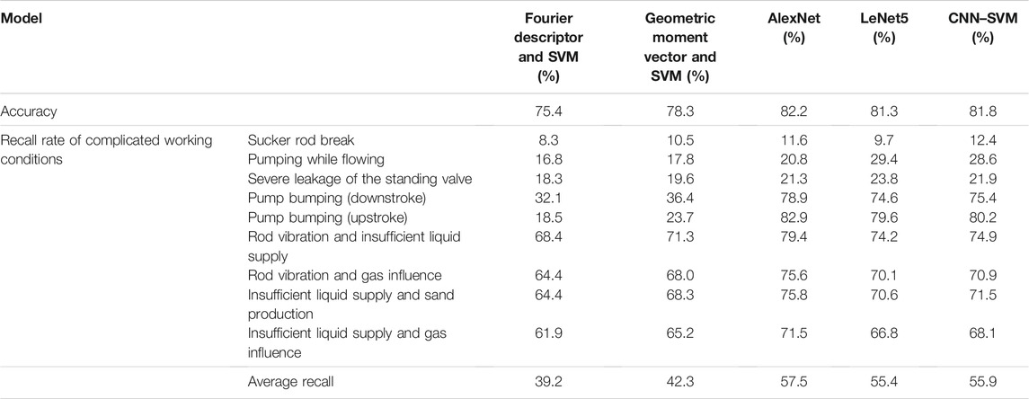
TABLE 1. Performance test results of each mainstream model.

Analyzing the data in Table 1, it can be found that when faced with a variety of working condition diagnostic tasks, the accuracy and recall rates of the SVM model based on feature extraction are low, and the performance of the model based on deep learning CNN is slightly improved. The two types of models have low recall rates for complicated working conditions such as sucker rod break, pumping while flowing, and serious leakage of standing valves and cannot meet the actual needs of the oil field. In order to solve the abovementioned problems, this article analyzes the reasons for the low recall rate of all models for complicated working conditions. A new dynamometer card preprocessing method is proposed; that is, multiple normalized scales are determined by a clustering analysis algorithm to obtain multiple normalized dynamometer cards of the original data, which add spatial features of dynamometer card, and using dynamometer card data at multiple time points to add time features. Based on this dynamometer card preprocessing method, we build four CNN architectures to test performance and compare with other models. We also explored the influence of hyperparameters of our method and demonstrated good results in field application.

Data Preprocessing Method of Dynamometer Card

The surface dynamometer card data collected at the oilfield production site is a sequence of polished rod load Y (kN) and displacement X (m) in a stroke, with 120 or 240 data points. The downhole working conditions are diagnosed according to the surface dynamometer card. The pump depth and stroke of different oil wells are different, so the position and size of the drawn dynamometer in the image coordinates are different. Before building the intelligent diagnosis model of SRP well, the first thing is performing the dynamometer card data preprocessing. Each dynamometer card data will be normalized to (0, 1) to obtain a fixed-size normalized dynamometer card to eliminate the difference in displacement and load. It makes the dynamometer card of the same working condition have the same shape feature, which is important for the algorithm model to learn the classification features. SVM and CNN are both excellent classification models; they have achieved good performance in many image classification scenarios, but perform poorly on the dynamometer card classification task, especially for some complicated working conditions, which are caused by improper data preprocessing methods. The traditional normalization method is based on the maximum and minimum of Y and X value of current dynamometer card data. We will analyze the shortcomings of this method and propose a new method.

The Normalization Method Based on the Maximum and Minimum of X and Y

Normalization is performed based on the maximum and minimum of X and Y, as shown in the following equations:

$\overline{X}=\frac{X-X_{min}}{X_{max}-X_{min}},(1)$

$\overline{Y}=\frac{Y-Y_{min}}{Y_{max}-Y_{min}}.(2)$

For each point in the dynamometer card data sequence, $\overline{X}$ and $\overline{Y}$ are the normalized displacement and load value. $X$ and $Y$ are the actual displacement and load value of the current dynamometer card data. $X_{min},X_{max}$, $Y_{min}, Y_{max}$ are the maximum and minimum values of displacement (m) and load (kN), which is called the normalized scale. It makes the different normalized dynamometer cards of one working condition show consistency in shape features, which is conducive to the model to better learn the classification features of this working condition and eliminate the noise in the data.

However, the dynamometer card of the working conditions such as sucker rod break, severe leakage of the standing valve, and pumping while flowing is the suspension point load change (see Figure 1A), and the position is different from that of the normal dynamometer card. Observing the normalized dynamometer cards of these working conditions (see Figure 1B), intuitively, they all present the same graphic features as the normal dynamometer cards, and the normalized dynamometer cards of different working conditions are confused and indistinguishable. This normalization method causes the inseparability of the data itself; therefore, no matter what model is used, the recall rate of sucker rod break, pumping while flowing, and serious leakage of standing valves working conditions are extremely low.

FIGURE 1

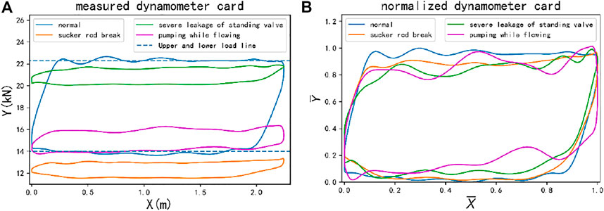
FIGURE 1. Normalized dynamometer card for the four working conditions.

For each SRP well, there is a group of theoretical $\left(Y_{\max }, Y_{\min }\right)$ of normal working conditions. When this is used as the normalized scale, the normalized dynamometer card is as shown in Figure 2.

FIGURE 2

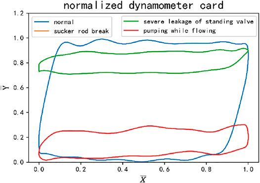
FIGURE 2. Use of theoretical load normalization.

This method retains the information about the position, shape, and size of the current dynamometer card relative to the normal dynamometer card. The normalized dynamometer cards of the two working conditions of pumping while flowing and serious leakage of standing valve are obviously separable. However, because the load $Y$ of the dynamometer card of the rod breakage condition is lower than $Y_{min}$, there is no geometric figure in the interval (0, 1) after normalization, resulting in the loss of image information; problems such as sensor failures and well shutdown operations can also cause loss of image information. Therefore, using theoretical $\left(Y_{\max }, Y_{\min }\right)$ alone as the normalization scale, it is still impossible to obtain a normalized dynamometer card with good separability for all working conditions.

Multi-Scale Dynamometer Card Normalization Based on Cluster Analysis

We simultaneously use the $\left(Y_{\max }, Y_{\min }\right)$ of actual load and theoretical load to obtain two normalized dynamometer cards as the input of the diagnostic model (Table 2). Through the complementarity between the feature information of the two normalized dynamometer cards, the dynamometer card for working conditions such as rod break, pumping while flowing, and severe leakage of the standing valve can be effectively distinguished (taking sucker rod break as an example, the first one is shown as the normal dynamometer card, and the second obtains a blank image, which means the rod breakage has occurred). Therefore, the data have classification separability.

TABLE 2

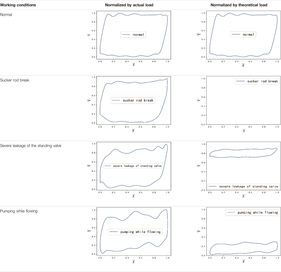
TABLE 2. Normalized dynamometer card combining two normalization methods.

The theoretical $\left(Y_{\max }, Y_{\min }\right)$ can be obtained in two ways. One is to calculate the polished rod load through a theoretical model. Due to the complexity of the downhole environment and fault working condition, the calculated theoretical load usually differs greatly from the actual theoretical load of the oil well. The second is to use the load measured by the dynamometer under normal working conditions and get the maximum and minimum values, but the oil well may be in abnormal working conditions at the beginning, and it is difficult to obtain effective value. In addition, $\left(Y_{\max }, Y_{\min }\right)$ of normal working conditions is a group values that changes with the production performance of the oil well, and it has different values in different periods; actually, we cannot get a group of constant values, and it needs to be updated frequently. Considering that the use of multiple normalization methods of different scales is essentially to extend the classification features of one dynamometer card data, a stable set of normalized scales is required. Therefore, a new normalization method of dynamometer card is proposed; in addition to normalizing the current dynamometer card data with the $\left(Y_{\max }, Y_{\min }\right)$ of the actual load, k different normalization scales are used to obtain another k normalized dynamometer cards, introducing enough classification features to enhance the separability of the data. For the current dynamometer card dataset, clustering algorithm (k-means) is used to obtain k normalized scales $u_i={\left(Y_{\max }, Y_{\min }\right)}_i,\text{i}\in [1,\text{k}]$.

The dataset for clustering is a collection of the vectors $\left(y_{\max },y_{\min }\right)$ of each dynamometer card data, and the number of clusters $k\in \left[\mathrm{2,30}\right]$ is selected for clustering. Figure 3 shows the cost function of clustering with different k values. The cost function is the sum of the degree of distortion of each class. The degree of distortion of each class is equal to the sum of the squares of the distance between the centroid of the class and its internal members. The larger the k is, the more normalized scale $u_i$ can be obtained. Figure 4 shows the cluster distribution of different k values. Each color represents a cluster, and the black dots in the cluster represent the mean vector (centroid) of each cluster, that is, the normalized scale. However, obtaining too many normalized dynamometer cards will increase the calculation amount of model training and prediction, but the enhancement of data separability is limited. In order to get a reasonable value of k, it is necessary to consider the cluster distribution of the cluster and the change trend of the cost function at the same time.

FIGURE 3

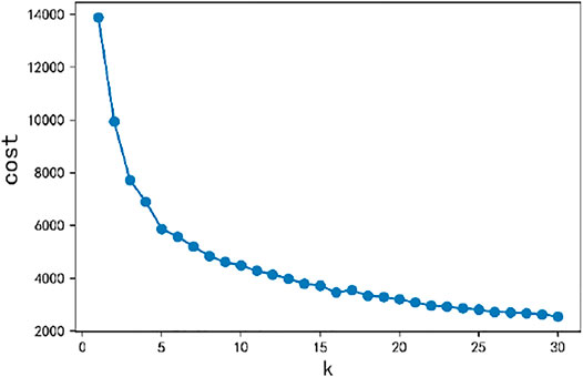
FIGURE 3. Cost function value of different k.

FIGURE 4

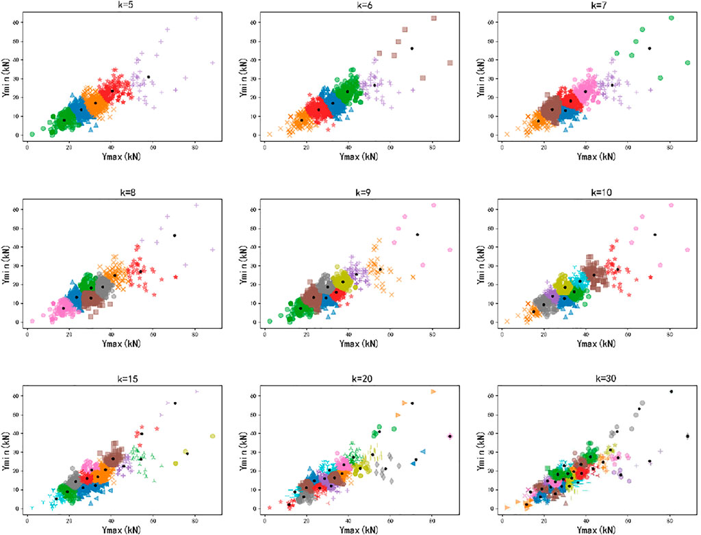
FIGURE 4. Cluster distribution of different k clusters.

According to the elbow rule, the value of the elbow of the cost function is selected as the reasonable value of k (the value of the cost function initially drops quickly, and the elbow starts to decline gradually). From Figure 3, it is observed that the elbow value is k = 5. Observing Figure 4, it is found that the clusters obtained by $k\in \left[\mathrm{5,10}\right]$ gradually become compact, and the quality of the cluster distribution is already good, which can obtain multiple effective normalization scales without excessively increasing the computational cost.

In addition, follow-up experiments verified the rationality of the k value range and explored the performance of the diagnostic model when selecting k = 15, 20, and 30 for normalization. Table 3 shows 11 normalized dynamometer cards for each working condition when k = 10. k0 represents the normalized dynamometer card obtained by $\left(Y_{\max }, Y_{\min }\right)$ of the actual load, and $\text{k}1\sim \text{k}10$ represent 10 normalized dynamometer cards obtained by $u_1\sim u_{10}$. From Table 3, although k0 of the three working conditions is very similar, it can be distinguished by combining k0–k10. Multi-scale normalization introduces multiple normalized dynamometer cards with significant shape differences to greatly enhance data quality, and it provides the relative variation features of the dynamometer card on the y-axis (for simplification, it is called spatial features). The model can extract spatial features from $\text{k}0\sim \text{k}10$, and this will help the model to recognize the originally inseparable working conditions, which improves the overall accuracy and the recall rate of complicated working conditions in the following experiments.

TABLE 3

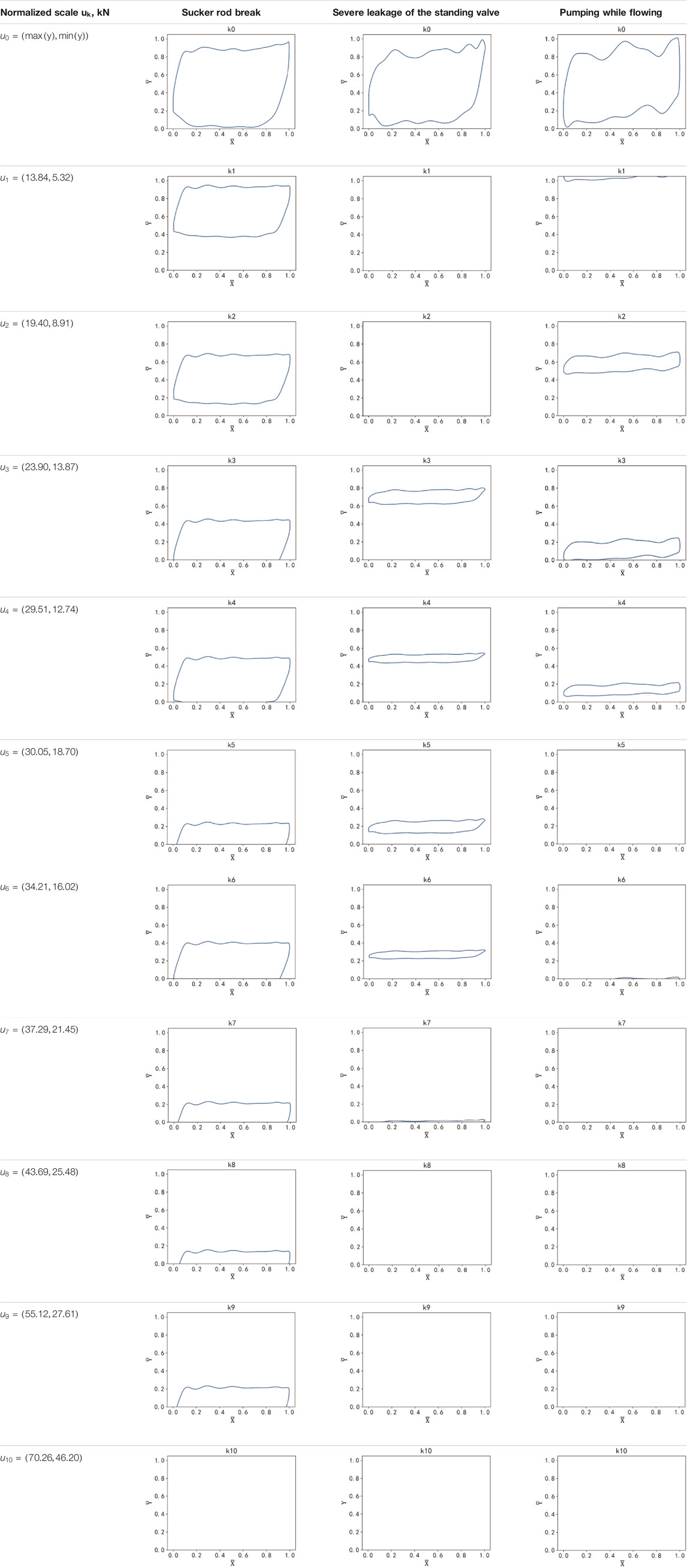
TABLE 3. Normalized dynamometer card of three working conditions (k = 10).

Adding Time-Series Features

During the production of SRP well, the current dynamometer cards of some working conditions are very similar, such as seriously insufficient liquid supply and pump bumping (upstroke), sucker rod break, and pumping while flowing. The traditional method uses the dynamometer card data at a single time point as the input data of the model, which is unable to distinguish effectively. The change trend of the dynamometer card of different working conditions is totally different; Figure 5 shows the change trend of dynamometer card of two different working conditions, and the change trend can also be used as a classification feature. In order to use the change trend features of dynamometer cards of different working conditions, the dynamometer cards at multiple time points are taken as the input data. In order to capture the short-term, mid-term, and long-term change features, in addition to the current dynamometer card, five dynamometer cards’ data 1T, 3T, 1 day, 10 days, and 30 days before are selected (T represents the data collection time interval of each dynamometer card, and 1 day means 24 h ago). The dynamometer card sequence contains the time-series change features of the working conditions, further enhances the data classification features, and provides a solid foundation for building a more robust model. m is used to represent the number of selected time points, and m can be dynamically adjusted independently according to the characteristics of the dataset being used; in this article, m = 5, and the time points are shown above.

FIGURE 5

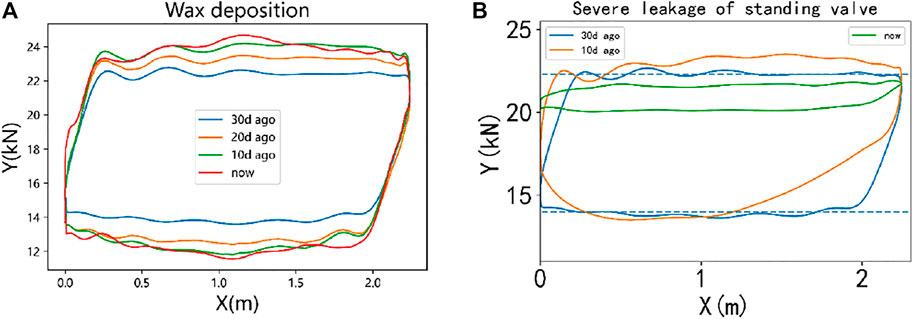
FIGURE 5. The change trend of dynamometer card of two different working conditions.

CNN-Based Diagnosis Model

In recent years, convolutional neural networks have been widely used in the field of image recognition, including many typical applications in the petroleum industry, such as offshore oil slick detection (Kubat et al., 1998; Corucci et al., 2010), reservoir physical property detection (Ahmadi 2015), using CNN as an automatic well test interpretation approach for infinite acting reservoirs (Liu et al., 2020), and pipeline network internal image detection (Loskutov et al., 2006; Smola et al., 2004). For the problem of dynamometer card classification, the use of convolutional neural networks does not require artificially designed feature extraction methods, and the performance is generally better than that of models such as SVM and BP. You can find the basic concepts and working principles of CNN in many studies (LeCun et al., 1998; Krizhevsky et al., 2012; Zeiler and Fergus, 2014); we will no longer give a basic introduction to it, and we will show how to build a CNN diagnostic model from three aspects in this article.

Preparing the Dataset

The data used in this study are collected from more than 1,200 sucker rod pumping wells in an oil field in China. One dynamometer card record is collected every 10 min for each oil well and stored in the database, and each record contains 200 points of load vs. displacement. The data from June 1, 2020, to July 31, 2020, are derived from the database and used as the original data for this study, and there are 864,576 data records in total. The original data preprocessing includes the following steps:

Step1: outlier data analysis: generally caused by the drift of the polished rod load, the slope of the dynamometer card curve changes suddenly. We calculate the slope between adjacent points and give a threshold. If the number of slopes exceeds the threshold and accounts for more than 1/3 of the total, the dynamometer card data are determined to be an outlier and deleted.

Step2: missing data analysis: for the missing data of load and displacement points, it is generally completed by interpolation of adjacent points. In this study, we only use interpolation to complete a single missing point, and data with two or more consecutive missing points will be deleted.

Step3: deleting similar data: in order to ensure the non-redundancy of data samples, we will delete similar dynamometer card data produced by the same oil well. The similarity function is often used to remove data duplication. The similarity calculation formula is as follows:

$R_{ij}=\exp \left(-\frac{1}{\delta }{\Vert x_i-x_j\Vert }^2\right),(3)$

where $R_{ij}$ is the similarity between any two samples of data, $\delta$ is the normalized parameter, $x_i$ and $x_j$ are any two groups in the sample data, $i,j=\mathrm{1,2},\dots \text{n}$, $\Vert ·\Vert$ is the 2-norm of the vector, and δ is calculated by

$\text{δ}={\displaystyle \sum }_{i=1}^n\left(max{D}_i-min{D}_i\right),(4)$

where $D_i$ is the value of the ith feature of the sample; for our sample data, it is the ith value of one dynamometer card. The similarity of load $R_{ij}^l$ and displacement $R_{ij}^d$ between two groups in the dynamometer card sample data is calculated; if the similarity is $R_{ij}^l+R_{ij}^d>\epsilon$, the two data contain most of the same information, then one is eliminated. Some data will be dropped in the abovementioned three steps, the amount of data dropped in each step is shown in Table 4, and most of the data is dropped in step 3.

TABLE 4

TABLE 4. The amount of data dropped in each step.

Step 4: drawing normalized dynamometer card: the dynamometer card data after three steps can be drawn into an image according to the data preprocessing method of dynamometer card, and each image be drawn with size 224 × 224 and line width 1 pixels. As we do not need the color information, the image adopts the gray-scale image format. Finally, a gray-scale pixel matrix of 224 × 224×(k + m +1) is obtained as the input of the model.

Once the normalized dynamometer card for each data is drawn, a team of experienced oilfield experts and field engineers begin to analyze and mark the working conditions corresponding to each data. According to the oil well production and operation records and the shape of the 16 normalized dynamometer cards, we divide the oil well working conditions in this dataset into 24 types, containing 20 single working conditions and 4 compound working conditions. The classification of working conditions and the amount of each type are shown in Table 5, a total of 19,510 samples.

TABLE 5

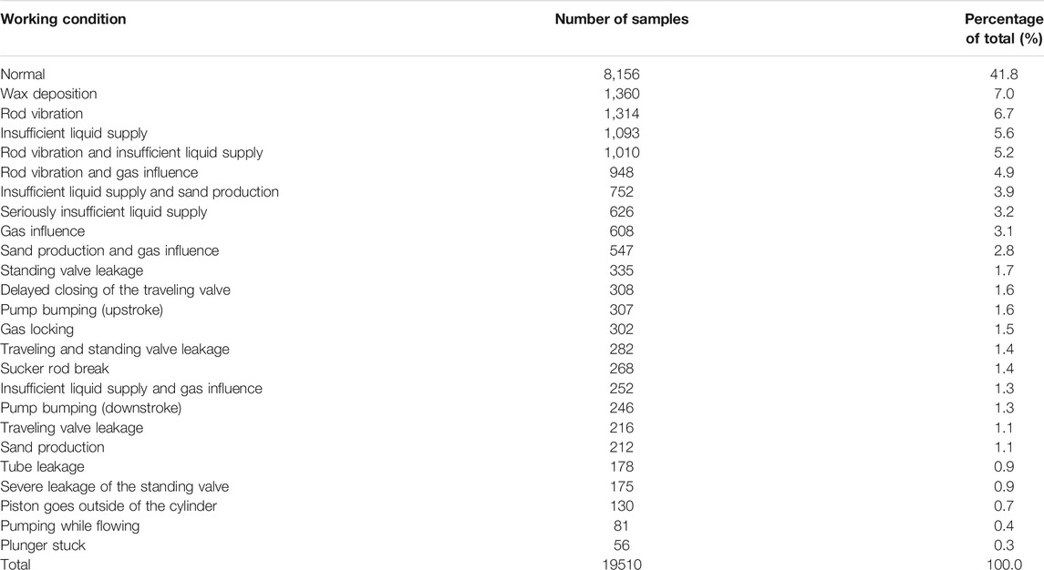
TABLE 5. Classification of the working conditions and the number of samples for each working condition.

From Table 5, we can find that the number of samples is unevenly distributed. Some common working conditions have a large number (accounting for the majority of the number of samples, called head classes), and some uncommon working conditions have a relatively small number of samples (accounting for the majority of the class, called tail classes). Such a sample dataset is called long-tail data. Models that directly use long-tail data to train tend to overfit the head data, thereby ignoring the tail class when predicting (Kang et al., 2019). This work adopts the method proposed by Tang et al. (2020) to optimize the long-tail effect, reduce the impact of long-tail data on the model performance, and make the model perform better in the prediction stage.

CNN Architecture Design

The classic deep CNNs include GoogLeNet (Szegedy et al., 2015), ResNet (He et al., 2016), and SENet (Hu et al., 2019). They have achieved “sota” results in the 1,000 image classification competition (ILSVRC: ImageNet Large Scale Visual Recognition Challenge). In deep learning, the optimal network architecture often depends on your goals and the characteristics of the dataset. For this reason, it is extremely difficult to design a new CNN with the optimal architecture. The differences between the working condition diagnosis task of SRP well and ILSVRC image classification are as follows: (1) the first only has 24 class, which is much less than the last; (2) the traditional image is represented by three RGB pixel matrices, so the model input has three channels, and the working condition diagnosis model input is multiple normalized dynamometer cards with (k + m+1) channels, which means that the model needs to process more feature maps at the input. What we know is that these classic models are a general paradigm and have achieved the best universal results. Therefore, this research will build a working condition diagnosis model based on these classic CNN architectures. Considering that our input data are multiple normalized indicator diagrams, what we need is to use a deep CNN with multiple input channels to extract the spatial and time-series features of the input data; the solution diagram is as shown in Figure 6, and $\text{k}0\sim \text{k}10$ are 11 pixel matrices of 11 normalized dynamometer cards from the multi-scale dynamometer card normalization process. Also, m dynamometer cards at different times are added, and those dynamometer cards are normalized by scale of the dynamometer card data 31 days ago. In this way, m normalized dynamometer cards have the relative change trend features with time.

FIGURE 6

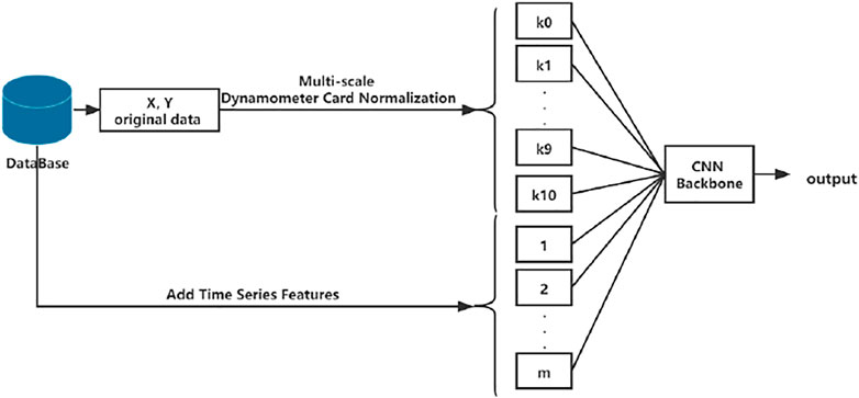
FIGURE 6. Preprocessing method combined with the CNN architecture solution diagram.

The following criteria should be followed when selecting the basic CNN backbone: (1) In the image recognition task, the residual architecture has become an important architecture commonly used, and the deep network built on this has excellent performance and fewer parameters (such as ResNet and SENet). (2) The identification of the dynamometer card is based on the features of the contour of the curve. Using the method in this work to obtain multiple normalized dynamometer card data has good separability, and a deep multi-channel residual network can be used to meet the needs of dynamometer card data classification. Based on the abovementioned considerations, this study constructed four CNN backbones as working condition diagnosis models: ResNet50, SE-ResNet50, ResNet50Ⅱ, and SE-ResNet50Ⅱ. The network architecture is shown in Table 6. ResNet50 and SEnet50 are the original architectures. ResNet50Ⅱ and SEnet50Ⅱ expand the number of channels in the middle layer of the entire network, which is twice the original number to cope with the increased input channels. The shapes and operations with specific parameter settings of a residual building block are listed inside the brackets, and the number of stacked blocks in a stage is presented outside. The inner brackets followed by fc indicate the output dimension of the two fully connected layers in an SE module (for detailed introduction of these modules, please refer to He K et al., 2016, and Hu J et al., 2018).

TABLE 6

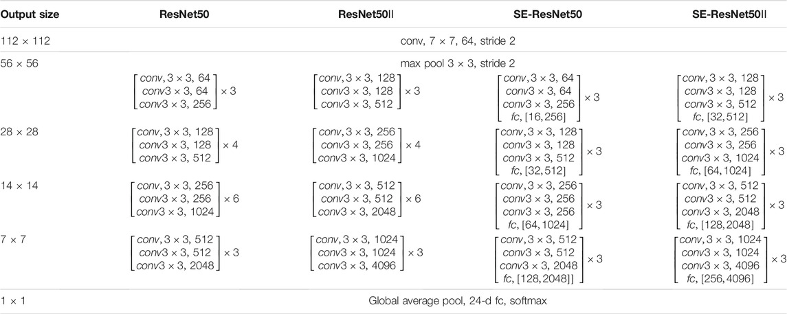
TABLE 6. Four kinds of network architecture parameters.

Training and Testing

The deep learning framework pytorch is used to implement four models. After each convolutional layer, batch normalization (BN, Ioffe et al., 2015) and activation function ReLu (Glorot et al., 2011) are used, and Eq. 5 is used to randomly initialize the network weight parameters.

$W_l=\text{R}\left({\text{d}}_l,{\text{d}}_{l-1}\right)\times \sqrt{\frac{2}{{\text{d}}_l}},(5)$

$W_l$ is the weight parameter of the lth layer, $d_l$ and $d_{l-1}$ are the number of neurons in the lth and previous layers, the R function generates a random function with a normal distribution between $[0,1]$.

The network is trained with 70% data, and 30% is tested. k is 10, and m is 5. The network model training parameters are as follows: Optimization method: Adam (betas = (0.9, 0.999), eps = 1e-08, and weight decay = 8e-4), batch size: 64, learning rate: 0.001, and epoch: 20. Due to alleviating the long-tail effect of the data, the method of Tang et al. (2020) is used to calculate loss and train the model. The SE-ResNet50 model is taken as an example. Figure 7 shows the accuracy vs. iterations, and Figure 8 shows the loss vs. epoch. The results show that the model is convergent for the dynamometer card dataset obtained by using multi-scale normalization. The Adam optimization method can obtain good results, and the accuracy rate on the test set can reach 95.6%. The model has a good generalization performance.

FIGURE 7

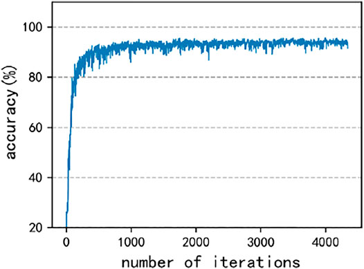
FIGURE 7. Cure of test accuracy vs. iterations.

FIGURE 8

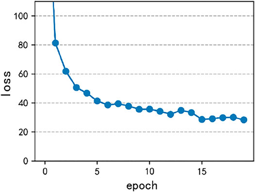
FIGURE 8. Curve of loss vs. epoch.

Experiment Analysis

The Influence of k Value on Model Performance

In the multi-scale normalization method, k determines the number and value of the normalization scale, which affects the performance of the diagnostic model. In order to optimize k, different k values are selected for normalization, and the same CNN backbone (SE-ResNet50) is used for training and testing. A total of nine values have been tested. Table 7 give the specific values of the experimental results, and Figure 9 shows its changing trend.

TABLE 7

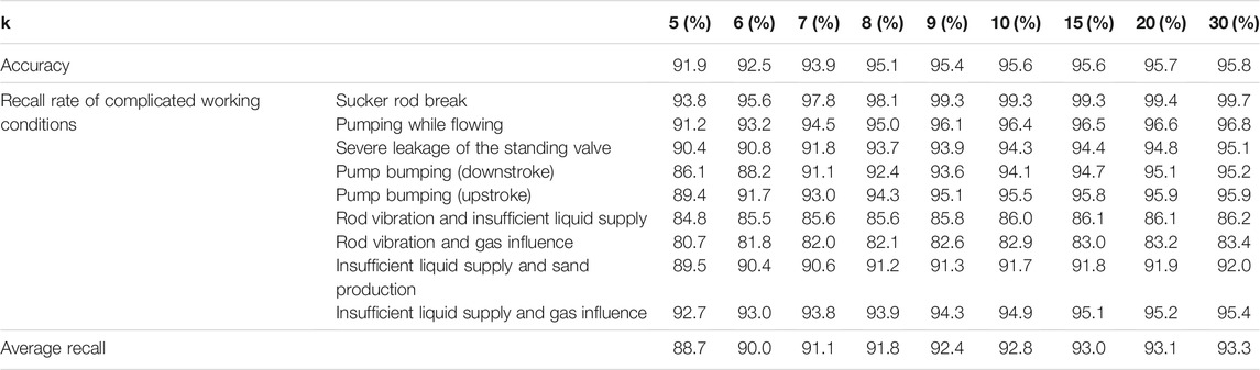
TABLE 7. Model performance under different multi-scale normalized k values.

FIGURE 9

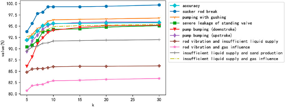
FIGURE 9. The change trend of model performance with k value.

From Figure 9 and Table 7, it can be found that various indicators show an upward trend with the increase of k, and the model performance is positively correlated with k. It shows that the increase in the k value helps the data introduce more feature information, enhance the separability of the data itself, and greatly improve the accuracy of the model and the recall rate of complicated working conditions. However, when the value of k is greater than 10, increasing k has a small improvement in model performance. Different datasets have different thresholds, and k = 10 is the most suitable value while taking into account the computational efficiency and performance.

The Influence of Time-Series Features on Model Performance

In this study, besides utilizing multi-scale normalization based on cluster analysis, the time-series features are also utilized. The influence of the time-series features is explored by setting up a control experimental group. We drop the time-series features, only use the k+1 feature map matrix as the input, and test its performance on the SE-ResNet50, and the recall rate of all working conditions with or without time-series features is shown in Table 8.

TABLE 8

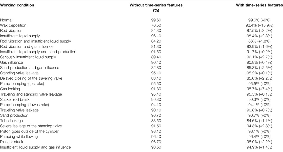
TABLE 8. Test results of different working conditions.

From Table 8, we can find that the recall rate of most working conditions has been improved with using time-series features, especially some working conditions have a long development term, such as wax deposition and gas locking. Because the dynamometer cards of these working conditions gradually change when they are finally formed, introducing time-series features by using dynamometer card data of multiple time points will help catch the change feature. In this way, the model will enhance the ability to recognize working conditions which have medium and long formation cycle.

Performance Comparison of Different Models

We have implemented six models using the dataset and dynamometer card preprocessing method in this article and using the 10-fold cross-validation method to compare the performance of different models, and k = 10 and m = 5 are set. This work adopts a radial basis function as the kernel function of SVM, and error penalty parameter C and kernel function parameter g are searched by particle swarm optimization (PSO, the best parameters C = 100, g = 0.01). The structure and hyper-parameter of AlexNet are same as those in the work of Krizhevsky A et al. (2017) except the input channel which is k+1 + m. Figure 10 and Table 9 give the experimental results. In Figure 10, every color bar represents a model’s recall rate of the listed working conditions in the horizontal axis and accuracy, and each color corresponds to one model. The experimental results are analyzed as follows: (1) using our data preprocessing method of dynamometer card greatly improves the overall accuracy and the recall rate. For example, the AlexNet model has increased by 9.4 and 28.8% which means that our method enhances the separability of the data itself, solves the inseparable defect of the data caused by the traditional normalization method, and is applicable to all models; (2) among the six models, the convolutional neural network is better than SVM, which means that, in the identification and classification of the dynamometer card, the automatic extraction of the dynamometer card graphic features by the convolutional neural network is better than the manually designed feature extraction method; and (3) the performance of SE-ResNet with both the residual module and the SE module is better than that of the ResNet with only the residual module. We think that the SE module improves the model’s sensitivity to channel features and can learn the relationship between different channels.

FIGURE 10

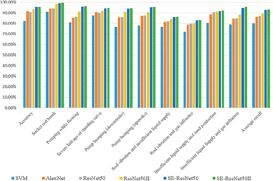
FIGURE 10. Accuracy and recall of different models.

TABLE 9

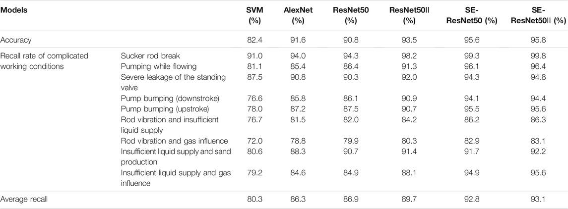
TABLE 9. Test results of different models.

Field Application Effect Evaluation

Starting from September 2020, the working condition diagnosis model has been applied in the field, and the deployment model is SE-ResNet50Ⅱ. From September 2020 to October 2020, there have been a total of 128 recalls of sucker rod break, severe leakage of the standing valve, pump bumping (upstroke), and pump bumping (downstroke). After the application of this model, the monthly average number of recalls of severe working conditions well has been greatly improved, as shown in Table 10.

TABLE 10

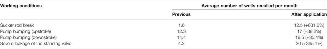
TABLE 10. Comparison of the monthly average number of wells recalled under severe working conditions.

The field application shows that the diagnosis model can accurately diagnose the working condition of each SRP well and timely help on-site personnel locate the oil well that has failed working condition, take correct countermeasures, and improve production efficiency. Since the model was launched, it has effectively improved the diagnosis accuracy and the recall rate of complicated working conditions. The overall accuracy rate can reach more than 95%, and the average recall rate for complicated working conditions is more than 90%, which meets the actual demand for intelligent diagnosis of working conditions on the oil field.

Conclusion

1) The defects of the traditional dynamometer card normalization method are demonstrated, and the experimental results show that the working condition diagnosis model with it will get poor results, not meeting actual needs.

2) We innovatively propose a new data preprocessing method of dynamometer card and give its workflow, using multiple normalized dynamometer cards of the original dynamometer card data as the model input can introduce more feature information and efficiently enhance the class separability of the data. It can improve the performance of all machine learning or deep learning models.

3) In 24 working condition diagnosis tasks, convolutional neural network is better than SVM. The network with extended middle layer width (ResNet50Ⅱ and SE-ResNet50Ⅱ) is slightly better than the original network structure (ResNet50 and SE-ResNet50). The SE-ResNet50 performs better, and we think that is because SE-ResNet50 learns the connection between different input channels.

k and m have different optimal values on different datasets. It is difficult to explore each different combination of k and m. The values given in this article are determined based on experience and experimental analysis and are suitable for most cases, and the influence of different m on the performance of the model is worth exploring. In the process of digital and intelligent development of the petroleum industry, using deep learning or data mining to analyze the internal relationship between data, we should first pay attention to the characteristics and quality of the dataset and then model structure and other optimization methods; this is what we want people to pay attention to through this article.

Data Availability Statement

The original contributions presented in this study are included in the article/Supplementary Material, further inquiries can be directed to the corresponding author.

Author Contributions

CT and PC are the proponents and researchers of the method of this paper, and PC is the code contributor of this research and the main writer of this paper. ZF provided guidance for the writing of this paper. ML, XA, QZ, and GF performed data collection and analysis for this article.

Funding

This research was supported by the National Natural Science Foundation of China (No. 51974327) and Key R&D Program of Anhui Province (No. 201904a05020028).

Conflict of Interest

Authors PC, XA, ML, and QZ are employed by CNPC ChangQing Petroleum. Author GF is employed by Beijing Yadan Petroleum Technology Development Co.

The remaining authors declare that the research was conducted in the absence of any commercial or financial relationships that could be construed as a potential conflict of interest.

Publisher’s Note

All claims expressed in this article are solely those of the authors and do not necessarily represent those of their affiliated organizations, or those of the publisher, the editors, and the reviewers. Any product that may be evaluated in this article, or claim that may be made by its manufacturer, is not guaranteed or endorsed by the publisher.

Abbreviations

ANN, artificial neural network, which simulates neuron activity with a mathematical model, is an information processing system based on imitating the structure and function of the brain neural network; CNN-SVM, a model composed of CNN and SVM; CNN is used to extract features, and SVM is used as classifier; SRP, sucker rod pumping, also referred to as “beam pumping,” provides mechanical energy to lift oil from the bottom-hole to surface; CNN, convolutional neural network. It is a kind of feedforward neural networks with depth structure including convolution calculation. It is one of the representative algorithms of deep learning; GBDT, gradient-boosted decision tree. It is a kind of decision tree with better performance; SVM, support vector machine. It is a kind of generalized linear classifier that classifies data in a binary way according to supervised learning; k, the number of normalized scales of dynamometer card, which is obtained by clustering algorithm; m, used to represent the number of dynamometer cards selected in different time points.

References

Abdalla, R., Ela, M. A. El., and El-Banbi, A. (2020). Identification of Downhole Conditions in Sucker Rod Pumped wells Using Deep Neural Networks and Genetic Algorithms. SPE Prod. Operations 35 (2), 435–447. doi:10.2118/200494-PA

CrossRef Full Text | Google Scholar

Ahmadi, M. A. (2015). Connectionist Approach Estimates Gas-Oil Relative Permeability in Petroleum Reservoirs: Application to Reservoir Simulation. Fuel 140, 429–439. doi:10.1016/j.fuel.2014.09.058

CrossRef Full Text | Google Scholar

Bangert, P., and Sharaf, S. (2019). “Predictive Maintenance for Rod Pumps,” in Paper presented at the SPE Western Regional Meeting. SPE-195295-MS. doi:10.2118/195295-MS

CrossRef Full Text | Google Scholar

Bezerra, M. A., Schnitman, L., Barreto Filho, M. D. A., Jose, A. M., and de Souza, F. (2009). Pattern Recognition for Downhole Dynamometer Card in Oil Rod Pump System Using Artificial Neural Networks. ICEIS 2, 351–355. doi:10.5220/0002000403510355

CrossRef Full Text | Google Scholar

Boguslawski, B., Boujonnier, M., Bissuel-Beauvais, L., Saghir, F., and Sharma, R. D. (2018). “IIoT Edge Analytics: Deploying Machine Learning at the Wellhead to Identify Rod Pump Failure,” in SPE Middle East Artificial Lift Conference and Exhibition. SPE-192513-MS. doi:10.2118/192513-MS

CrossRef Full Text | Google Scholar

Corucci, L., Nardelli, F., and Cococcioni, M. (2010). “Oil Spill Classification from Multi-Spectral Satellite Images: Exploring Different Machine Learning Techniques,” in Remote Sensing of the Ocean, Sea Ice, and Large Water Regions 7825: 782509. International Society for Optics and Photonics. doi:10.1117/12.864556

CrossRef Full Text | Google Scholar

de Lima, F. S., Guedes, L. A., and Silva, D. R. (2012). Comparison of Border Descriptors and Pattern Recognition Techniques Applied to Detection and Diagnose of Faults on Sucker-Rod Pumping System. Digital Image Process.. doi:10.5772/33245

CrossRef Full Text | Google Scholar

Eickmeier, J. R. (1967). Diagnostic Analysis of Dynamometer Cards. J. Pet. Technol. 19 (1), 97–106. SPE-1643-PAh. doi:10.2118/1643-PA

CrossRef Full Text | Google Scholar

Glorot, X., Bordes, A., and Bengio, Y. (2011). Deep Sparse Rectifier Neural Networks. Proc. fourteenth Int. Conf. Artif. intelligence Stat. 15, 315–323. Available at: https://proceedings.mlr.press/v15/glorot11a.html.

Google Scholar

He, K., Zhang, X., Ren, S., and Sun, J. (2016). “Deep Residual Learning for Image Recognition,” in 2016 IEEE Conference on Computer Vision and Pattern Recognition (CVPR), 770–778. doi:10.1109/CVPR.2016.90

CrossRef Full Text | Google Scholar

Hu, J., Shen, L., Albanie, S., Sun, G., and Wu, E. (2020). Squeeze-and-Excitation Networks. IEEE Trans. Pattern Anal. Mach Intell. 42 (8), 2011–2023. doi:10.1109/TPAMI.2019.2913372

PubMed Abstract | CrossRef Full Text | Google Scholar

Ioffe, S., and Szegedy, C. (2015). “Batch Normalization: Accelerating Deep Network Training by Reducing Internal Covariate Shift,” in International conference on machine learning, 448–456. Available at: https://ui.adsabs.harvard.edu/abs/2015a-rXiv150203167I.

Google Scholar

Kang, B., Xie, S., Rohrbach, M., Yan, Z., Gordo, A., Feng, J., et al. (2019). Decoupling Representation and Classifier for Long-Tailed Recognition. arXiv preprint arXiv:1910.09217. Available at: https://ui.adsabs.harvard.edu/abs/2019arXiv191009217K.

Google Scholar

Krizhevsky, A., Sutskever, I., and Hinton, G. E. (2017). ImageNet Classification with Deep Convolutional Neural Networks. Commun. ACM 60 (6), 84–90. doi:10.1145/3065386

CrossRef Full Text | Google Scholar

Kubat, M., Holte, R. C., and Matwin, S. (1998). Machine Learning for the Detection of Oil Spills in Satellite Radar Images. Machine Learn. 30 (2), 195–215. doi:10.1023/A:1007452223027

CrossRef Full Text | Google Scholar

Lecun, Y., Bottou, L., Bengio, Y., and Haffner, P. (1998). Gradient-based Learning Applied to Document Recognition. Proc. IEEE 86 (11), 2278–2324. doi:10.1109/5.726791

CrossRef Full Text | Google Scholar

Li, K., Gao, X.-w., Yang, W.-b., Dai, Y.-l., and Tian, Z.-d. (2013a). Multiple Fault Diagnosis of Down-Hole Conditions of Sucker-Rod Pumping wells Based on Freeman Chain Code and DCA. Pet. Sci. 10 (3), 347–360. doi:10.1007/s12182-013-0283-4

CrossRef Full Text | Google Scholar

Li, K., Gao, X., Tian, Z., and Qiu, Z. (2013b). Using the Curve Moment and the PSO-SVM Method to Diagnose Downhole Conditions of a Sucker Rod Pumping Unit. Pet. Sci. 10 (1), 73–80. doi:10.1007/s12182-013-0252-y

CrossRef Full Text | Google Scholar

Liu, X., Li, D., Yang, J., Zha, W., Zhou, Z., Gao, L., et al. (2020). Automatic Well Test Interpretation Based on Convolutional Neural Network for Infinite Reservoir. J. Pet. Sci. Eng. 195, 107618. doi:10.1016/j.petrol.2020.107618

CrossRef Full Text | Google Scholar

Loskutov, V. E., Matvienko, A. F., Patramanskii, B. V., and Shcherbinin, V. E. (2006). The Magnetic Method for In-Tube Nondestructive Testing of Gas and Oil Pipelines: The Past and the Present. Russ. J. Nondestruct Test. 42 (8), 493–504. doi:10.1134/S1061830906080018

CrossRef Full Text | Google Scholar

Smola, A. J., and Schölkopf, B. (2004). A Tutorial on Support Vector Regression. Stat. Comput. 14 (3), 199–222. doi:10.1023/B:STCO.0000035301.49549.88

CrossRef Full Text | Google Scholar

Szegedy, C., Liu, W., Jia, Y., Sermanet, P., Reed, S., Anguelov, D., et al. (2015). “Going Deeper with Convolutions,” in 2015 IEEE Conference on Computer Vision and Pattern Recognition (CVPR), 1–9. doi:10.1109/CVPR.2015.7298594

CrossRef Full Text | Google Scholar

Tang, K., Huang, J., and Zhang, H. (2020). Long-tailed Classification by Keeping the Good and Removing the Bad Momentum Causal Effect. Available at: https://ui.adsabs.harvard.edu/abs/2020arXiv200912991T.

Google Scholar

Wang, X., He, Y., Li, F., Wang, Z., Dou, X., Xu, H., et al. (2021). A Working Condition Diagnosis Model of Sucker Rod Pumping wells Based on Deep Learning. SPE Prod. Operations 36 (2), 317–326. doi:10.2118/205015-PA

CrossRef Full Text | Google Scholar

Xu, P., Xu, S., and Yin, H. (2007). Application of Self-Organizing Competitive Neural Network in Fault Diagnosis of Suck Rod Pumping System. J. Pet. Sci. Eng. 58 (1), 43–48. doi:10.1016/j.petrol.2006.11.008

CrossRef Full Text | Google Scholar

Yu, Y., Shi, H., and Mi, L. (2013). Research on Feature Extraction of Indicator Card Data for Sucker-Rod Pump Working Condition Diagnosis. J. Control. Sci. Eng.. doi:10.1155/2013/605749

CrossRef Full Text | Google Scholar

Zeiler, M. D., and Fergus, R. (2014). Visualizing and Understanding Convolutional Networks. Computer Vis. – ECCV 8689, 818–833. doi:10.1007/978-3-319-10590-1_53

CrossRef Full Text | Google Scholar