A Novel Method for Determining Geophone Orientations From Zero-Offset VSP Data Constrained by Scalar Field

In vertical seismic profile (VSP) acquisition, the orientation of the three-component geophones in a borehole is often not aligned due to random rotation of the wireline receiver array. Knowing the geophone orientation is crucial for rotating the waveforms back to the position where the geophones are assumed to be aligned. This procedure is critical in three-component VSP data processing as it provides the correct wavefields for subsequent VSP data imaging and inversion. For zero-offset or near zero-offset VSP measurements, the direct P-wave propagates nearly vertically, and the horizontal geophones receive only a small fraction of the direct P-wave energy. The first-arrival in the horizontal component data is often of low signal-to-noise ratio (SNR). As a result, it is difficult to apply conventional first-arrival–based methods for obtaining accurate geophone orientations. On the other hand, a seismic event comprising individual waveform would achieve maximum correlation if all corresponding geophones are aligned. The geometric characteristics, that is, the slope and continuity of a seismic event in the vector wavefield are the same with those of the modules of the vector wavefield. The latter, also known as the scalar wavefield, can be used for scanning geophone orientations based on waveform correlation. In this study, we propose to use the scalar field to extract the slope of seismic events. The orientation of the individual geophone was calculated with the constraint of the slope. We use both synthetic and field data to demonstrate the effectiveness and applicability of the proposed method. The results show that the new method can provide wavefields of horizontal component VSP data with much higher accuracy and resolution.

Introduction

The orientations of the geophones are hard to control in the borehole, which leads to random rotation of horizontal geophones in the three-component VSP acquisition. A universal coordinate system is required for processing vector field data of different acquisition positions. The inconsistent orientation of geophones not only leads to inconsistent coordinate systems of geophone data but also cause poor continuity of the events of the received vector wavefield (DiSiena et al., 1984). This makes the processing and analysis of VSP data difficult. Accurate information about the orientations of geophones is critical for transforming the geophone coordinate systems with Z-, X-, and Y-component axes into a consistent acquisition coordinate system with Z-, R- (radial of shot-receiver), and T-component (transverse of shot-receiver) axes (Liu et al., 2003), which is also the foundation of subsequent vector wave separation (Lu et al., 2018, 2019).

In the methods for determining geophone orientation, the most common one is based on the first-arrival of P-wave. In a VSP acquisition, the polarization direction of first-arrival is parallel to the direction of the shot-to-receiver array. Therefore, the direction of the geophone can be determined by analyzing the polarization characteristics of first-arrivals. Methods related to first-arrival include signal correlation (Becquey and Dubesset, 1990; Guevara and Stewart, 2001), matrix transform (Greenhalgh and Mason, 1995; Hendrick and Hearn, 1999; Li and Yuan, 1999; Park et al., 2004), principal component analysis (Michaels 2001), polarization analysis (Knowlton and Spencer, 1996; Oye and Ellsworth, 2005), energy maximization (Lagos and Velis, 2019), and eigenvector and eigenvalue method (Zaręba and Danek, 2018). Menanno et al. (2013) pointed out that the geophone orientation in a walkaround VSP can be estimated more accurately by using a 3D velocity model and allowing for ray bending. The aforementioned methods rely on accurate picking of P-wave first-arrival. The advantages of these methods are fewer data input and fast evaluation. They are commonly suitable for VSP data with strong first-arrivals. However, for zero-offset or near zero-offset VSP measurements, the direct P-wave propagates vertically to the subsurface sediments, leading to weak energy of horizontal components. Furthermore, due to attenuation and dispersion of seismic waves, the amplitude decay of signals becomes more pronounced with increasing depth. In addition, noises in field data may also smear the weak direct P-wave signals. Therefore, in practice, it is difficult to obtain the orientations of geophones by simply analyzing the first-arrival signals.

There also exist a group of methods that do not make use of the first-arrival signals. Zeng and McMechan proposed the relative angle method (Zeng and McMechan, 2006; Katou et al., 2018), where the orientations of the geophones are obtained by averaging the relative azimuths calculated from all shot points. Huo et al. (2021) determined the relative orientations between the sensor pairs by maximizing the waveform coherence along all the traces for the seismic events. These methods are especially suitable for the cases where multiple resources are located at different positions. However, for single-shot data, it is not easy to collect the statistics of relative angles. Grigoli et al. (2012) proposed a complex linear least-squares method to derive relative and absolute geophone orientations. Krieger and Grigoli (2015) used the eigenvectors of a real symmetric matrix to form quaternions and performed coordinate rotation. Zhu et al. (2018) developed a least squares method and combined an attitude and heading reference system for the orientation of all geophones in geographical coordinates. In essence, these methods are used to rotate the signal of one geophone to the coordinate system of another geophone. This requires that the distance between the geophones is much smaller than the wavelength and presence of limited number of geophones so that the time difference between detectors can be ignored. However, when the number of geophones increases, the non-zero time difference can lead to cumulative errors.

On the other hand, the geometric characteristics (slope and continuity) of the seismic events in vector wavefields are consistent with those of scalar fields (i.e., module of vector field). If the geophones are aligned, meaning each component of the geophone points to the same direction, the seismic event would achieve maximum correlation. Therefore, this important information can be used as a constraint to scan the orientations of geophones based on waveform correlation. In this study, we propose to divide the shot gather data into shallow and deep parts because in the shallow part, the P-waves travel a shorter distance and experience less attenuation. For this situation, the direct first-arrivals can still be evident and applied to determine geophone orientations. In the deep part, based on the scalar field of the horizontal component, the slopes of events are obtained. With the constraint of this attribute, we extract the accurate orientations of geophones. This is followed by reconstructing the correct horizontal component wavefields. Both synthetic and field VSP data were used to demonstrate the applicability of the proposed method.

Methods

Orientation Determination Based on First-Arrival Eigenvalue Method

Signals received by the geophone at shallow depth show the characteristics of approximate linear polarization. This is because with shorter travel distance, the first-arrival amplitude experiences less attenuation and hence, the signal-to-noise ratio (SNR) is high. The conventional eigenvalue methods that use first-arrivals can be directly used to calculate the geophone orientations. First, we need to determine the average value within the time window of first-arrivals. This can be achieved by using the following equations:

$\{\begin{array}{c}\overline{x_i\left(t\right)}=\frac{1}{N}{\displaystyle \sum _{t=t_{fi}-wt}^{t_{fi}+wt}{x}_i\left(t\right)}\\ \overline{y_i\left(t\right)}=\frac{1}{N}{\displaystyle \sum _{t=t_{fi}-wt}^{t_{fi}+wt}{y}_i\left(t\right)}\end{array}.(1)$

Then, a covariance matrix is created as follows:

$M=\left[\begin{array}{cc}{\displaystyle \sum _{t=t_{fi}-wt}^{t_{fi}+wt}{\left(x_i\left(t\right)-\overline{x_i\left(t\right)}\right)}^2}& {\displaystyle \sum _{t=t_{fi}-wt}^{t_{fi}+wt}\left(x_i\left(t\right)-\overline{x_i\left(t\right)}\right)\left(y_i\left(t\right)-\overline{y_i\left(t\right)}\right)}\\ {\displaystyle \sum _{t=t_{fi}-wt}^{t_{fi}+wt}\left(x_i\left(t\right)-\overline{x_i\left(t\right)}\right)\left(y_i\left(t\right)-\overline{y_i\left(t\right)}\right)}& {\displaystyle \sum _{t=t_{fi}-wt}^{t_{fi}+wt}{\left(y_i\left(t\right)-\overline{y_i\left(t\right)}\right)}^2}\end{array}\right],(2)$

where x_i(t) and y_i(t) are original signals of x and y components, t_fi is the first-arrival at the ith geophone, and wt is the half-length of the time window. The largest eigenvector of the covariance matrix Eq. 2 is associated with the polarization direction and represents the deflection angle. The ratio of the minimum and maximum eigenvalues is the polarizability (Jolliffe, 1986). Therefore, the R- and T-component data can be calculated based on the deflection angle αs follows:

$\left[\begin{array}{c}{\mathit{R}}_{\mathit{i}}\left(\mathit{t}\right)\\ {\mathit{T}}_{\mathit{i}}\left(\mathit{t}\right)\end{array}\right]=\left[\begin{array}{cc}\mathit{sin}{\mathit{\alpha }}_{\mathit{s}}& \mathit{cos}{\mathit{\alpha }}_{\mathit{s}}\\ -\mathit{cos}{\mathit{\alpha }}_{\mathit{s}}& \mathit{sin}{\mathit{\alpha }}_{\mathit{s}}\end{array}\right]\left[\begin{array}{c}{\mathit{x}}_{\mathit{i}}\left(\mathit{t}\right)\\ {\mathit{y}}_{\mathit{i}}\left(\mathit{t}\right)\end{array}\right]\mathrm{..}(3)$

Orientation Scanning Constrained by Scalar Field

For deep geophones, it is difficult to determine the geophone orientation through the first-arrivals with low signal-to-noise ratio. The vector wavefield comprising X- and Y-components cannot reflect the slope and continuity of events due to random geophone orientations. However, the module of the vector wavefield, that is, the scalar wavefield is independent of the geophone orientations. This feature enables the scalar field of horizontally polarized waves (mainly S-wave and possibly P-wave) to reflect the characteristics of the slope and continuity of the events.

In the first step, we calculate the scalar field by taking the modules of the horizontally polarized wave, that is, the ith horizontal components x_i(t) and y_i(t):

$S_i\left(t\right)=\sqrt{x_i{\left(t\right)}^2+y_i{\left(t\right)}^2}.(4)$

The seismic events associated with the scalar field of the horizontal components are usually continuous. The corresponding slope indicates the apparent velocity of the seismic wave. The slope can be used as a constraint for scanning geophone orientation. A fast method to calculate the slope of events is to use the negative ratio of the x- and t-direction (i.e., time-depth domain) scalar field data with Hilbert and inverse Fourier transformations (Liu et al., 2015):

$k_{i,t}=\mathit{tan}{\mathit{\sigma }}_{i,t}\approx \mathit{tan}\left(-\frac{FF{T}^{-1}\left[H_{HT}{\left(x\right)}_{i,t}\right]}{FF{T}^{-1}\left[H_{HT}{\left(t\right)}_{i,t}\right]}\right),(5)$

where σ is the dip angle of events. The next step is to choose an appropriate time window for orientation scanning. It is unnecessary to choose the slope of all sampling points as the constraint because this increases computation cost. Instead, it can be optimized by selecting the time window where the sample point attains maximum correlation in the scalar field. The correlation between trace i and previous M traces can be calculated by

$C_i\left(t\right)=\frac{{\displaystyle \sum _{\tau =-w}^w{\displaystyle \prod _{m=0}^M{S}_{i-m}\left(t-\tau -m\mathrm{\Delta }x{k}_{i,t}\right)}}}{\sqrt{{\displaystyle \prod _{m=0}^M{\displaystyle \sum _{\tau =-w}^w{S}_{i-m}^2\left(t-\tau -m\mathrm{\Delta }x{k}_{i,t}\right)}}}},\left(\mathit{t}-\mathit{\tau }-\mathit{m}\mathrm{\Delta }\mathit{x}{\mathit{k}}_{\mathit{i},\mathit{t}}\in \left(0,\mathit{n}\right)\right),(6)$

where Δx is the interval of geophones, and n is sample number. The maximum correlation of trace i is determined through

$C_i\left(t_{i\mathit{max}}\right)=\mathit{max}\left\{C_i\left(t\right)\right\}.(7)$

Setting the orientation of the horizontal geophone as α_d, the signals of R- and T-components can be rotated as follows:

$\left[\begin{array}{c}{R}_i\left(t\right)\\ T_i\left(t\right)\end{array}\right]=\left[\begin{array}{cc}\mathit{sin}{\alpha }_d& \mathit{cos}{\alpha }_d\\ -\mathit{cos}{\alpha }_d& \mathit{sin}{\alpha }_d\end{array}\right]\left[\begin{array}{c}{x}_i\left(t\right)\\ y_i\left(t\right)\end{array}\right].(8)$

The objective function of orientation scanning is the sum of the correlation of R- and T-components constrained by the slope of events in the scalar field:

$C_{RTi}\left({\alpha }_d\right)=\frac{{\displaystyle \sum _{\tau =-w}^w{\displaystyle \prod _{m=0}^M{R}_{i-m}\left(t_{i\mathit{max}}-\tau -m\mathrm{\Delta }x{k}_{i,t}\right)}}}{\sqrt{{\displaystyle \prod _{m=0}^M{\displaystyle \sum _{\tau =-w}^w{R}_{i-m}^2\left(t_{i\mathit{max}}-\tau -m\mathrm{\Delta }x{k}_{i,t}\right)}}}}+\frac{{\displaystyle \sum _{\tau =-w}^w{\displaystyle \prod _{m=0}^M{T}_{i-m}\left(t_{i\mathit{max}}-\tau -m\mathrm{\Delta }x{k}_{i,t}\right)}}}{\sqrt{{\displaystyle \prod _{m=0}^M{\displaystyle \sum _{\tau =-w}^w{T}_{i-m}^2\left(t_{i\mathit{max}}-\tau -m\mathrm{\Delta }x{k}_{i,t}\right)}}}},i\ge H_0,(9)$

where H₀ is the number of geophones in the shallow region. Because the orientations of the shallow geophones are obtained by the eigenvalue method, the shallow trace data need to satisfy the following conditions: 1) the polarizability is small enough; 2) the SNR of the first-arrival is high, which is the basis of the eigenvalue method to obtain relatively accurate results. When the objective function attains the maxima, α_dmax is the orientation of the ith trace, that is,

$C_{RTi}\left({\alpha }_{d\mathit{max}}\right)=\mathit{max}\left\{C_{RTi}\left({\alpha }_d\right)\right\}.(10)$

The workflow is summarized in Figure 1. First, we pick the first-arrival based on the Z-component data. This is followed by dividing the VSP shot gather into shallow and deep parts based on the polarizations of the first-arrivals. Then, the orientations of geophones in the shallow and deep parts are obtained by the eigenvalue and scalar field methods, respectively. Finally, the horizontal components are rotated based on the orientation, and accurate R- and T-component data can be obtained.

FIGURE 1

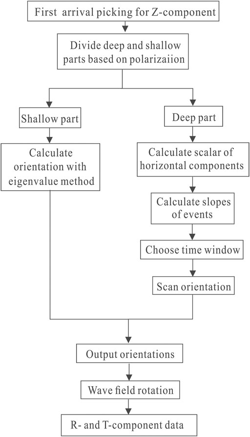
FIGURE 1. Flowchart of the scalar field method for determining geophone orientations.

Data Example

In this section, both synthetic and field data are used to examine the effectiveness of the proposed workflow. To model the VSP data, we establish a horizontal 4-layer model, the parameters of which are given in Table 1. The VSP acquisition is as follows: the geophones are located at the depth of 500–1,400 m in a well with an interval of 5 m. The shot point is located at the surface with a zero-offset. Figure 2 shows the single-shot record simulated using finite difference elastic wave simulation. As indicated by the red arrow, the first-arrivals of the P-wave received by geophones at greater depth show weak amplitude. In the abovementioned example, the geophones are aligned, and the data are noise-free. In the second example, the noises are added with a signal-to-noise ratio of 10dB to the simulated data. In addition, a random rotation is assigned to each geophone to mimic the actual VSP acquisition in a well. The data with noises and random geophone rotation are shown in Figure 3. As indicated by the red arrow, we can barely identify the first-arrivals which are masked by noises. Therefore, it is almost impossible to determine the polarization direction of the first-arrival. The continuity of the wavefields also deteriorates.

TABLE 1

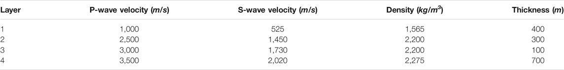
TABLE 1. Parameters of the model.

FIGURE 2

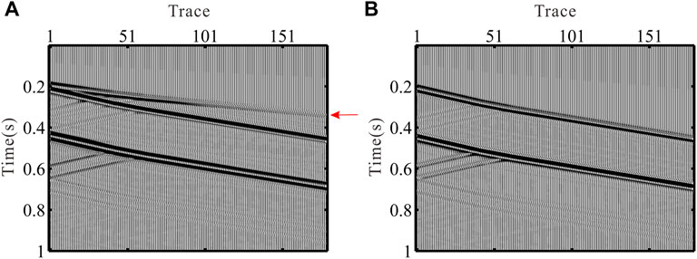
FIGURE 2. Synthetic VSP data without noises and the geophones are aligned. (A) X-component. (B) Y-component.

FIGURE 3

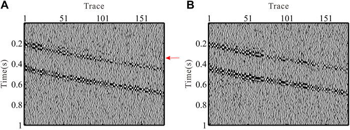
FIGURE 3. Synthetic VSP data with noises and random geophone rotations. (A) X- and (B) Y-component.

The scalar field of the horizontal components and the slope of events are calculated based on Eq. 4 and Eq. 5, respectively. The results are shown in Figure 4. To fully test the scalar field method based on slope constraint, we set the shallow part as the first five traces and the parameter M in Eq. 6 and Eq. 9 as 5. Using Eq. 8 and Eq. 9, the X- and Y-component data are rotated to R- and T-components based on the results of the orientation scanning. The R- and T-components are shown in Figures 5C,D. For comparison, we also present the results from the eigenvalue method in Figures 5A,B. As shown in Figures 5C,D, the orientation scanning is constrained by scalar field results in the R/T components that closely resemble the original data (see Figure 2). In Figures 5A,B, the noises persist in the data, and the eigenvalue method produces rotated data with poor continuity of the events.

FIGURE 4

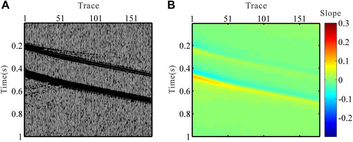
FIGURE 4. (A) Scalar field of the horizontal components of synthetic VSP data and (B) corresponding slope of the scalar field.

FIGURE 5

FIGURE 5. (A) R- and (B) T-component VSP data generated by the largest eigenvector of covariance matrix (C). R- and (D) T-component generated by the proposed method.

In order to evaluate the accuracy of the two methods, we apply the eigenvalue and the scalar field methods to synthetic data with different noise levels. We take the absolute value of the difference between the predicted and the accurate orientations of the geophones as the error. In Figure 6, the blue and red histograms show the error distributions associated with the eigenvalue and the scalar field methods, respectively. The error is expressed in terms of angle degree. The SNR of the data in Figures 6A,B, Figures 6C,D, and Figures 6E,F are 2, 15, and 5dB, respectively. Figure 6 clearly shows that the scalar field method is superior to the eigenvalue method especially when the data are of poor quality (with a low SNR). The scalar field method is efficient in predicting the geophone orientation angle, regardless of the noise level. In contrast, the eigenvalue method becomes less effective in handling noisy data.

FIGURE 6

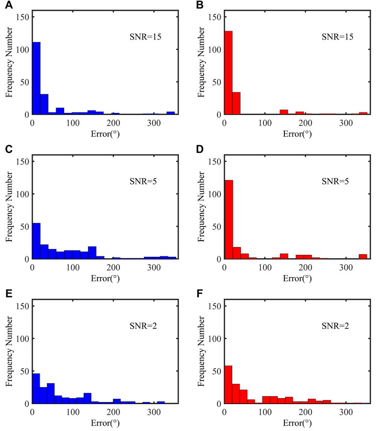
FIGURE 6. Errors in orientation results of all geophones for the synthetic data. The SNRs of (A–B), (C–D), and (E–F) are 15, 5, and 2dB. The left column shows the results obtained from the eigenvalue method, and the right column shows the results obtained using the scalar field method.

Finally, the proposed scalar field method is applied to a field zero-offset VSP dataset shown in Figures 7A,B. The borehole geophones are located between 2,800 and 3,600 m in a well with a spacing of 10 m. Figures 7C,D show the scalar field of the horizontal components and the slope of events calculated using Eq. 4 and Eq. 5, respectively. We first show results associated with the eigenvalue method in Figures 8A,B. We can see that there are some abrupt amplitude changes and phase reversals in the R/T components. This leads to poor continuity of the reflection events. For the same purpose as the model test, we set the shallow part as first five traces and M as 5. The results from the scalar field method are shown in Figures 8C,D. It is evident that the SNR of VSP data becomes much higher, and the continuity of events is significantly improved.

FIGURE 7

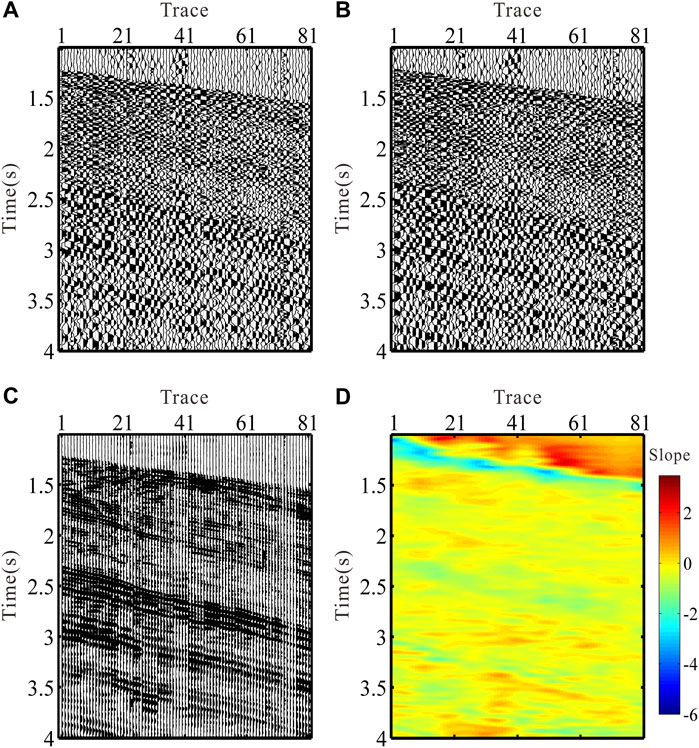
FIGURE 7. Field zero-offset VSP data before rotation. (A) X-component. (B) Y-component. (C) Scalar field of the horizontal components data. (D) Corresponding slope of the scalar field.

FIGURE 8

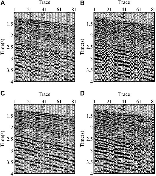
FIGURE 8. Field seismic data after rotation. (A) R- and (B) T-component VSP data generated by the eigenvalue method. (C) R- and (D) T-component generated by the scalar field method.

In order to compare the wavefield recovery of the two methods in more detail, we selected different types of wavefields for comparison, as shown in Figure 9. The left and right columns are the results of the eigenvalue method and the scalar field method, respectively. Figures 9A,B show the first-arrivals. The results shown in the right column have better continuity. Figures 9C,D show the upgoing wavefield. The results shown in the right column contain the upgoing wavefield (the slopes of the upgoing and downgoing wavefield events are opposite) as shown by the red quadrilateral in Figure 9D. Figures 9E,F show the first-arrivals of shear wave, and it is obvious that the continuity of the results on the right is better. The comparison clearly shows that the developed workflow is efficient in determining the geophone orientations. The latter forms the basis for an accurate R/T component wavefield recovery.

FIGURE 9

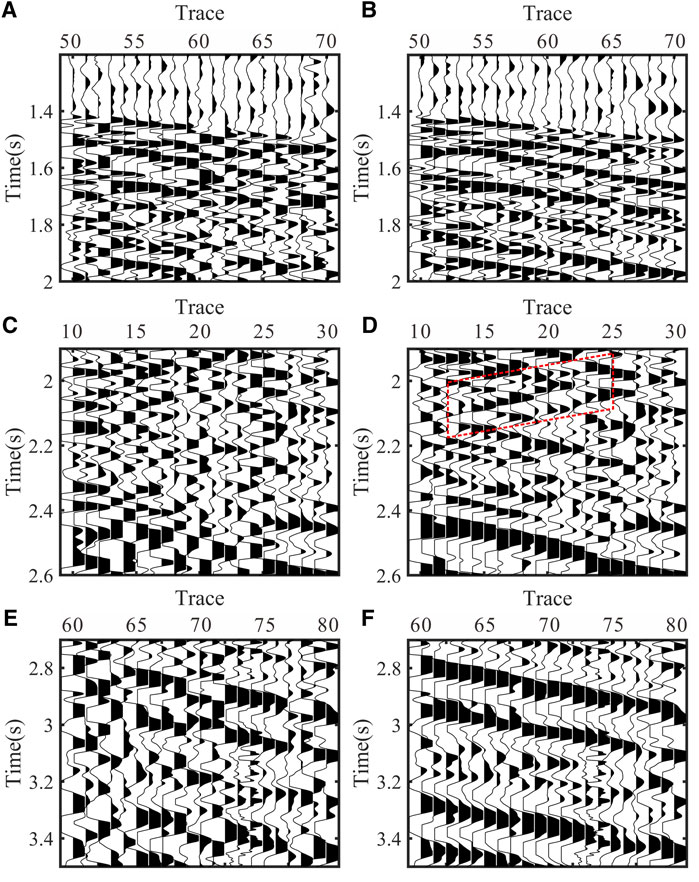
FIGURE 9. Typical wavefields of field seismic data after rotation. (A), (C), and (E): VSP data generated by the eigenvalue method. (B), (D), and (F): VSP data generated by the scalar field method.

Discussion

In the deep layer, the orientations of the geophones are calculated one by one from the first to the last. As the objective function in Eq. 9, the orientation of the current geophone is determined by the signals of the previous M traces, and it is necessary to ensure that there are enough traces in the shallow layer when calculating the first trace in the deep layer. Therefore, the number of geophones (H₀) in the shallow part should be greater than M. In addition, the orientation scanning of the current trace is constrained by the previous M trace data. Such a procedure increases the stability of the algorithm compared with the calculation that uses only two adjacent traces. Especially for the VSP acquisition with a long geophone array, the scalar field method produces less cumulative error and is less sensitive to noises. However, the proposed method is based on the accurate results of shallow geophone orientations. If the shallow results are not accurate, it is also difficult to obtain accurate results using the scalar field method. This shows that the implementation of this method is not independent.

We have demonstrated that this method is effective for zero-offset VSP data. Moreover, it is expected that the method can also be applied to non–zero-offset VSP data. This is because the slope of the scalar field in any VSP survey system can be used in constraining the rotation of horizontal components. On the other hand, since seismic waves may not propagate along the Z-component direction of the geophones, the horizontal and vertical components can receive both P- and S-wave signals. After geophone orientation correction, the pure P- and S-waves shall be extracted from horizontal and vertical components for the subsequent PP and PS imaging/inversion. This will be a subject of future research.

Conclusion

Aiming at the problem that the first-arrivals of zero-offset VSP data can be weak and contaminated by noises, we propose a scalar field method for accurately determining the geophone orientations. The method uses the scalar field of the horizontal component as a constraint in the orientation scanning process and yields reliable orientation angles of geophones. To achieve this, we need to divide the shot gather data into shallow and deep parts based on the polarization characteristics of the first-arrivals. Shallow data can be processed by the eigenvalue method. For deep data, we calculate the scalar field of the horizontal component. The slopes of events are obtained by the Hilbert transform of the scalar field data. Making use of these slopes, orientation scanning, which is the sum of the correlation between X- and Y-components, can be carried out in a constrained time window. The synthetic and field data applications show that the scalar field method is efficient in determining geophone orientations from zero-offset VSP data.

Data Availability Statement

The original contributions presented in the study are included in the article/Supplementary Material, further inquiries can be directed to the corresponding author.

Author Contributions

YY, QQ, and ZW developed the method and performed the applications. HZ supervised the findings of this study. All authors discussed the results and contributed to the final manuscript.

Funding

This study was funded by the National Natural Science Foundation of China (Grant Numbers, 41904113 and 42074160) and the Sichuan International Science and Technology Innovation Cooperation Program (Grant Numbers, 2021YFH0050 and 2021YFG0257).

Conflict of Interest

The authors declare that the research was conducted in the absence of any commercial or financial relationships that could be construed as a potential conflict of interest.

Publisher’s Note

All claims expressed in this article are solely those of the authors and do not necessarily represent those of their affiliated organizations, or those of the publisher, the editors, and the reviewers. Any product that may be evaluated in this article, or claim that may be made by its manufacturer, is not guaranteed or endorsed by the publisher.

References

Becquey, M., and Dubesset, M. (1990). Three‐component Sonde Orientation in a Deviated Well. Geophysics 55 (10), 1386–1388. doi:10.1190/1.1442786

CrossRef Full Text | Google Scholar

DiSiena, J. P., Gaiser, J. E., Corrigan, D., and Toksöz, M. N. (1984). “Horizontal Components and Shear Wave Analysis of Three-Component VSP Data,” in Vertical Seismic Profiling, Part B: Advanced Concepts. Editors M. N. Toksöz, and R. R. Stewart (London: Geophysical Press Ltd.), 177–235.

Google Scholar

Greenhalgh, S. A., and Mason, I. M. (1995). Orientation of a Downhole Triaxial Geophone. Geophysics 60 (4), 1234–1237. doi:10.1190/1.1443852

CrossRef Full Text | Google Scholar

Grigoli, F., Cesca, S., Dahm, T., and Krieger, L. (2012). A Complex Linear Least-Squares Method to Derive Relative and Absolute Orientations of Seismic Sensors. Geophys. J. Int. 188 (3), 1243–1254. doi:10.1111/j.1365-246X.2011.05316.x

CrossRef Full Text | Google Scholar

Guevara, S. E., and Stewart, R. R. (2001). “3‐C Geophone Orientation and Wave Modes Polarization,” in SEG Technical Program Expanded Abstracts (Tulsa, Oklahoma, USA: Society of Exploration Geophysicists), 799–801. doi:10.1190/1.1816754

CrossRef Full Text | Google Scholar

Hendrick, N., and Hearn, S. (1999). Polarisation Analysis: What Is it? Why Do You Need it? How Do You Do it? Exploration Geophys. 30 (4), 177–190. doi:10.1071/eg999177

CrossRef Full Text | Google Scholar

Huo, Y., Zhang, W., Zhang, J., and Yang, H. (2021). Using Microseismic Events to Improve the Accuracy of Sensor Orientation for Downhole Microseismic Monitoring. Geophys. Prospecting 69 (6), 1167–1180. doi:10.1111/1365-2478.13099

CrossRef Full Text | Google Scholar

Jolliffe, I. T. (1986). Principal Component Analysis. New York: Springer.

Google Scholar

Katou, M., Abe, S., Saito, H., and Sato, H. (2018). Reciprocal Data Acquisition and Subsequent Waveform Matching for Integrated Onshore-Offshore Seismic Profiling. Geophys. J. Int. 212 (1), 509–521. doi:10.1093/gji/ggx374

CrossRef Full Text | Google Scholar

Knowlton, K. B., and Spencer, T. W. (1996). Polarization Measurement Uncertainty on Three‐component VSP. Geophysics 61 (2), 594–599. doi:10.1190/1.1443985

CrossRef Full Text | Google Scholar

Krieger, L., and Grigoli, F. (2015). Optimal Reorientation of Geophysical Sensors: A Quaternion-Based Analytical Solution. Geophysics 80 (2), F19–F30. doi:10.1190/GEO2014-0095.1

CrossRef Full Text | Google Scholar

Lagos, S., and Velis, D. (2019). A Simple Energy-Based Strategy for Sensor Orientation in Borehole Microseismic Monitoring. J. Geophys. Eng. 16 (1), 85–91. doi:10.1093/jge/gxy007

CrossRef Full Text | Google Scholar

Li, X.-Y., and Yuan, J. (1999). Geophone Orientation and Coupling in Three-Component Sea-Floor Data: a Case Study. Geophys. Prospecting 47 (6), 995–1013. doi:10.1046/j.1365-2478.1999.00160.x

CrossRef Full Text | Google Scholar

Liu, C., Chen, C.-L., Wang, D., Liu, Y., Wang, S.-Y., and Zhang, L. (2015). Seismic Dip Estimation Based on the Two-Dimensional Hilbert Transform and its Application in Random Noise Attenuation. Appl. Geophys. 12 (1), 55–63. doi:10.1007/s11770-014-0474-4

CrossRef Full Text | Google Scholar

Liu, E., Queen, J. H., Li, X. Y., Chapman, M., Maultzsch, S., Lynn, H. B., et al. (2003). Observation and Analysis of Frequency-dependent Anisotropy from a Multicomponent VSP at Bluebell-Altamont Field, Utah. J. Appl. Geophys. 54 (3–4), 319–333. doi:10.1016/j.jappgeo.2003.01.004

CrossRef Full Text | Google Scholar

Lu, J., Shi, Y., and Yang, C. (2018). Vector Wave Separation in Anisotropic media and its Application. Chin. J. Geophys. 61 (8), 3310–3323. doi:10.6038/cjg2018L0387

CrossRef Full Text | Google Scholar

Lu, J., Wang, Y., Chen, J., and Sun, P. (2019). P- and S-Mode Separation of Three-Component VSP Data. Exploration Geophys. 50 (4), 430–448. doi:10.1080/08123985.2019.1606205

CrossRef Full Text | Google Scholar

Menanno, G., Vesnaver, A., and Jervis, M. (2013). Borehole Receiver Orientation Using a 3D Velocity Model. Geophys. Prospect. 61, 215–230. doi:10.1111/j.1365-2478.2012.01106.x

CrossRef Full Text | Google Scholar

Michaels, P. (2001). Use of Principal Component Analysis to Determine Down-Hole Tool Orientation and Enhance SH-Waves. Jeeg 6, 175–183. doi:10.4133/JEEG6.4.175

CrossRef Full Text | Google Scholar

Oye, V., and Ellsworth, W. L. (2005). Orientation of Three-Component Geophones in the San Andreas Fault Observatory at Depth Pilot Hole, Parkfield, California. Bull. Seismological Soc. America 95 (2), 751–758. doi:10.1785/0120040130

CrossRef Full Text | Google Scholar

Park, J., Kim, W., and Baag, C.-E. (2004). Phase Identification Analysis Using Directionality and Rectilinearity Functions in Three Component Seismograms. Geosci. J. 8 (2), 199–209. doi:10.1007/BF02910196

CrossRef Full Text | Google Scholar

Zaręba, M., and Danek, T. (2019). Correction to: VSP Polarization Angles Determination: Wysin-1 Processing Case Study. Acta Geophys. 67 (2), 737. doi:10.1007/s11600-019-00277-3

CrossRef Full Text | Google Scholar

Zeng, X., and McMechan, G. A. (2006). Two Methods for Determining Geophone Orientations from VSP Data. Geophysics 71 (4), V87–V97. doi:10.1190/1.2208935

CrossRef Full Text | Google Scholar

Zhu, Y., Lin, J., Zhao, F., Chen, Z., Sun, F., and Lv, H. (2018). A Least Squares Method Based on Quaternions to Derive Absolute Orientation of Geophones with AHRS. J. Geophys. Eng. 15 (6), 2614–2624. doi:10.1088/1742-2140/aadd2f

CrossRef Full Text | Google Scholar