Vertical Variations of Submesoscale Motions Between New Jersey Shelf and Bermuda

Based on the measurements from the Oleander Project, the behaviors of submesoscale motions are examined in the area between New Jersey Shelf and Bermuda. The vertical variation of Rossby number, the kinetic energy in the submesoscale range, and the power law of kinetic energy spectra suggest that submesoscale motions are mainly confined within the surface mixed layer with seasonality that is strong in winter and weak in summer. Besides, submesoscale motions with no significant seasonality were also found beneath the surface mixed layer, which could reach 500 m depth. A possible explanation is that the drastically varying flows in the Gulf Stream and mesoscale eddy periphery could generate strong lateral shear throughout their influence depth, which is favorable for breaking the geostrophic balance and causing submesoscale motions beneath the surface mixed layer.

Introduction

The ocean dynamics vary in a wide range of spatial–temporal scales. The planetary scale motions, including large-scale and mesoscale motions, are dominated by planetary rotation and density stratification (Mensa et al., 2013). At these scales, flows are under the balance of Coriolis force and lateral pressure gradient, and the planetary rotation plays a more important role than advection; thus, their Rossby number $Ro={\varsigma }_z/f$ is much smaller than 1, where ζ_z is the vertical relative vorticity and f is the planetary vorticity. Planetary scale motions are the main energy source for the ocean, for example, 90% oceanic kinetic energy stored in mesoscale eddies (Fu et al., 2010). On the contrary, the microscale motions, with spatial scale in O(1) mm, are dominated by advection and diffusion, which are fully three-dimensional turbulent flows (Mensa et al., 2013) and have Ro >> 1. The kinetic energy reaching here would be dissipated into heat eventually (Kolmogorov et al., 1991); therefore, the microscale motions are the main energy sink for the ocean. Between these two scales, there are motions called submesoscale motions, with spatial scale ranging from O(100) m to O(10) km and in the form of fronts, filaments, and eddies (Thomas et al., 2008; McWilliams, 2016). For submesoscale motions, planetary rotation and advection are equally important, resulting in Ro ∼ O(1), implying submesoscale motions are ageostrophic.

During the past years, submesoscale motions have become a hotspot of research and been mainly investigated by numeral simulations (Levy et al., 2001; Capet et al., 2008; Molemaker et al., 2015; Callies, 2018). Due to the high-level spatial resolution requirement of the research on submesoscale motions, studies based on satellite measurements and in situ observations are still rare. Pollard and Regier (1992) observed strong vertical velocities of up to 40 m/day and surface-trapped eddies in submesoscale (40 km) during frontal experiments, and they suggested that submesoscale eddies play a crucial role in property transports between the ocean surface and the interior. Based on high-resolution MODIS sea surface temperature and Chlorophyll-a product, Taylor and Ferrari (2011) found that submesoscale fronts could re-stratify the well-mixed surface layer and cause phytoplankton explosive bloom. Apparently, due to their re-stratification of mixed layer and strong vertical motions, submesoscale motions could explain a big part of the ocean phytoplankton production (Levy et al., 2001; Klein and Lapeyre, 2009; Mahadevan, 2016), which provides a probability to explain that the mesoscale motions cannot maintain the observed productivity level in a basin-scale (Oschlies, 2002; 2008; Martin and Pondaven, 2003). Through theoretical studies and numeral simulations, the properties and dynamics of submesoscale motions are gradually revealed. Submesoscale motions exist in the ocean surface mixed layer widely (Fox-Kemper et al., 2008; Gula et al., 2014; Qiu et al., 2014), mainly driven by frontogenesis and mixed layer instabilities (Lapeyre et al., 2006; Boccaletti et al., 2007; McWilliams, 2016), and they are characterized by a significant seasonality being active in winter and weak in summer (Callies et al., 2015; Buckingham et al., 2016). Due to their ageostrophic behavior, submesoscale motions are capable of breaking the geostrophic balance and transferring energy forward from mesoscale to microscale dissipation, hence making much contribution to energy cascade in the ocean (McWilliams, 2016).

Recently, some studies indicate that the weakly stratified layer over sloping topography can drive the active submesoscale field by baroclinic instability resulting from the release of available potential energy, which is caused by the elevated abyssal mixing in the deep ocean, or the Ekman adjustment of currents on slope (Wenegrat et al., 2018). These bottom boundary layer baroclinic instabilities are comparable to those in the surface mixed layer, suggesting this instability is energetic and widespread in the global oceans. Similar to the surface scenario, the bottom submesoscale eddies would re-stratify the bottom mixed water and thus maintain the elevated abyssal turbulence mixing, which play a crucial role in modulating the overturning circulation (Callies, 2018). Moreover, submesoscale motions in the bottom boundary layer also have an influence on the cross-shelf exchanges (Gula et al., 2015) and generation of long-lived submesoscale coherent vortices (Molemaker et al., 2015).

Submesoscale motions have been shown to be existing in both surface and bottom boundary layers in many regions. Are there submesoscale motions in the ocean interior, such as beneath the mixed layer? In this study, we present observed submesoscale motions beneath the mixed layer and make a reasonable explanation about their mechanism. The manuscript is organized as follows. In Materials and Methods, we briefly introduce the data source and data processing methods. In Results, we show results of submesoscale motions within the surface mixed layer, and then we discuss submesoscale motions occurring beneath the mixed layer and propose a possible explanation in Discussion. A brief summary in Conclusion is followed at last.

Materials and Methods

Oleander Project

The data used in this study are mainly from the Oleander Project (Flagg et al., 1998), named by a container vessel CMV Oleander. This project was initiated in 1977 by the University of Rhode Island, Stony Brook State University of New York, the NOAA Northeast Fisheries Science Center, and the NOAA Atlantic Oceanographic Meteorological Laboratory, aiming to collect high-resolution upper-layer oceanographic data including ocean currents, temperature, salinity, and surface carbon dioxide in the dynamic and climatically important region, the Northwest Atlantic between New Jersey and Bermuda. The CMV Oleander repeats round-trips (red dashed line in Figure 1) between Port Elizabeth, New Jersey, and Hamilton, Bermuda, across the continental shelf near New Jersey, the Slope Sea, the Gulf Stream path (marked by thick white arrows in Figure 1), and a part of the Sargasso Sea. In this study, the current and temperature measurements are used. The horizontal current measurements began in 1992 by a shipboard narrow-band 150 kHz RD Instruments acoustic Doppler current profiler (ADCP) with limited vertical range to the upper 200 m. In 2005, a 75 kHz ADCP was installed, extending the depth range to ∼600 m in the Sargasso Sea. To better explore the hydrography under the mixed layer, the measurements from 2005 to 2016 were used in this study. The ADCP data were downloaded from the data retrieval website (http://po.msrc.sunysb.edu/Oleander) with 8 m vertical resolution, which is the usual vertical bin-size of those ADCP measurements, and the horizontal resolutions vary between 0.7 and 2 km, which are interpolated to 1.5 km along the sections. Besides, the temperature profiles measured by an eXpendable BathyThermograph (XBT) during 2013–2016 are used to calculate the mean mixed layer depth, which have a vertical resolution of 2 m.

FIGURE 1

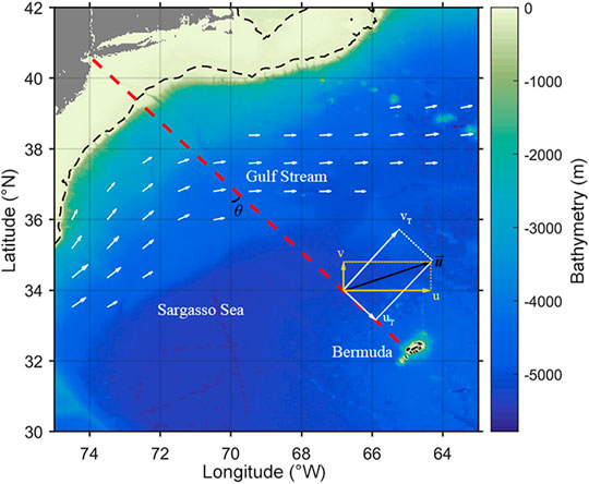
FIGURE 1. Bathymetry of the region where the Oleander Project was conducted (the black dashed line is the 100 m isobath) and its ideal course track (the red dashed line). The thick white arrows are strong surface flow revealing the Gulf Stream path, the thin arrows are diagrams of the velocity transformation, the yellow arrows are the original meridional and zonal velocities, and the white arrows are the along-track and across-track velocities after transformation. The transformation is based on the angle of the track and the latitude, θ. The bathymetry data are taken from ETOPO2 (https://ngdc.noaa.gov/mgg/global/etopo2.html), and the sea surface velocity data are from ECCO Version 4 release 4 (https://ecco-group.org/products-ECCO-V4r4.htm, Forget et al., 2015; ECCO Consortium et al., 2021b, a).

Flow Transformation, Decomposition, and Wavenumber Spectra

We investigate the submesoscale motions by examining the Ro values, in which the vertical relative vorticity is calculated as ${\varsigma }_z=\partial v/\partial x-\partial u/\partial y$, where (u, v) and (x, y) are the velocity components and grid spacing in zonal and meridional directions, respectively. Although the velocities $\overrightarrow{u}$ measured by the ADCP are expressed as u and v, however, the Oleander Project measurements were conducted along a linear section, and this section was not along the zonal or meridional direction but had an angle θ to the meridional direction (Figure 1). Therefore, the zonal and meridional velocities (u, v) are transformed into along-track and across-track velocities (u_T, v_T) for further calculations and analyses (sketched by thin white, black, and yellow arrows in Figure 1):

$\begin{array}{l}{\mathit{u}}_{\mathit{T}}=\mathit{u}\cdot \mathit{sin}\mathit{\theta }-\mathit{v}\cdot \mathit{cos}\mathit{\theta },\\ {\mathit{v}}_{\mathit{T}}=\mathit{u}\cdot \mathit{cos}\mathit{\theta }+\mathit{v}\cdot \mathit{sin}\mathit{\theta }.\end{array}$

And the vertical relative vorticity is expressed as ${\varsigma }_z=\partial v_T/\partial l$, where l is the spatial spacing along the sections. As the lateral gradient of u_T in the cross-section direction is neglected, the accuracy of the relative vorticity calculation deeply relies on the section orientation relative to the flow direction, with the relative vorticity being accurate when the section is perpendicular to the flow and being more and more inaccurate as their angle becomes smaller. The main flow in the study area is the Gulf Stream, which intersects with the sections with angles greater than 70° (Figure 6); the other part of flows we care in this study is the mesoscale eddies, especially those near the eddy periphery, which are basically orthogonal to the sections (Figure 8E). Besides, to ensure the credibility of the results, we calculate the mean ratio of v_T and u_T of each section; only those greater than 2.1 are further analyzed, which is equivalent to an intersection angle threshold of 65°.

Besides, the kinetic energy in the submesoscale range $\text{SKE}=1/2\left(u_s^2+v_s^2\right)$ would be elevated if there are energetic submesoscale motions, where (u_s, v_s) are velocity components in the submesoscale range. The (u_s, v_s) can be separated from the total velocity by using a reasonable high-pass filter in space, with the cutoff wavelength distinguishing submesoscale motions from large-scale and mesoscale motions in the study area. This cutoff wavelength is determined via Rossby deformation radius R = Nh/f, where N is the buoyancy frequency, h is the mixed layer depth, and f is the Coriolis parameter. Taking the local values of N ≈ 10⁻² s⁻¹, h ≈ 100 m, and f ≈ 10⁻⁴ s⁻¹, we applied R = 10 km to the high-pass filter and obtained submesoscale velocities (u_s, v_s).

As submesoscale motions are intrinsically different from meso/large-scale motions in dynamic sense, they show a different power law in the spectral domain. Both observations and simulations show that the spectra of energetic submesoscale motions obey a power law of k⁻² instead of k⁻³ when geostrophic motions dominate (Capet et al., 2008; Callies et al., 2015), which is also a criterion to validate the existence of submesoscale motions. Energy spectra of along-track velocities u_T and across-track velocities v_T are computed as

${\mathit{S}}^{\mathit{u}}\left(\mathit{k}\right)=\langle {\left|{\widehat{\mathit{u}}}_{\mathit{T}}\left(\mathit{k}\right)\right|}^2\rangle ,{\mathit{S}}^{\mathit{v}}\left(\mathit{k}\right)=\langle {\left|{\widehat{\mathit{v}}}_{\mathit{T}}\left(\mathit{k}\right)\right|}^2\rangle ,$

where k is the wavenumber, the caret denotes Fourier transform, and $\langle \cdot \rangle$ denotes the depth average. Besides to inspect the spectral slopes, the spectra can also be used to examine submesoscale energy levels during different periods and depths (Callies et al., 2015).

Results

Submesoscale Motions Within the Mixed Layer Revealed by Rossby Number

The Ro along the section during 10–15 December 2015 (case 201512) and 26–31 May 2016 (case 201605) is shown in Figure 2, which reveal the typical vertical variations of submesoscale motions in the study area in different seasons. Generally, there are “traditional cognitive” submesoscale motions that are energetic in winter and confined within the surface mixed layer; however, some Ro∼1 patches are found in 300 and 450 m in both periods, suggesting the occurrence of submesoscale motions beneath the surface mixed layer.

FIGURE 2

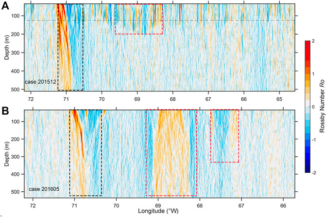
FIGURE 2. Longitude–depth variations of Ro in case 201512 (A) and case 201605 (B). The gray dashed line marks the mean mixed layer depth 125 m in winter. The black dashed boxes mark the Gulf Stream position, while the red dashed boxes represent the position of mesoscale eddies that generate/influence submesoscale motions.

The most distinguished Ro ∼ 1 patches are found near 71°W in both cases with depth ranging from the surface to about 350 m, which fall out of the scope of this subsection and will be discussed later. Our focus here are those elevated Ro values east of 70°W in case 201512, which are mainly confined within the upper 130 m with maximum and mean |Ro| being 2.2 and 0.7, respectively. These elevated Ro patches have a typical horizontal length scale of ∼3 km, coinciding with the spatial scale of submesoscale motions. The temperature profiles measured by XBTs (Figure 3) show the local mixed layer depth (determined by the threshold method with ΔT = 0.2°C, following de Boyer Montégut et al. (2004)) is about 125 m in winter, consistent with the depth ranges of elevated Ro. All these results indicate the ubiquity of energetic submesoscale motions within the surface mixed layer in case 201512, which was conducted in winter. On the contrary, apart from the areas influenced by the Gulf Stream and mesoscale eddies (black and red dashed boxes in Figure 2), |Ro| exceeding 0.1 can barely be found in case 201605, indicating the decline of submesoscale motions in summer.

FIGURE 3

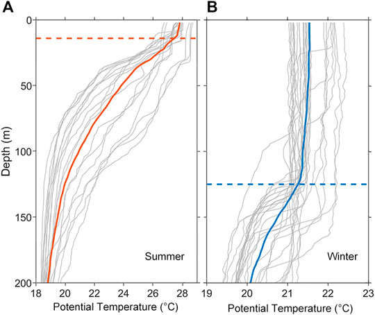
FIGURE 3. Upper 200 m potential temperature profiles measured by XBTs. (A) Profiles measured in summer (represented by July): the light gray curves are actual profiles measured individually, the orange solid curve is their average, and the dashed orange line marks the mean surface mixed layer depth in summer, 14 m. (B) Profiles measured in winter (represented by December): the light gray curves are actual profiles measured individually, the blue solid curve is their average, and the dashed blue line marks the mean surface mixed layer depth in winter, 125 m.

Spectra and Submesoscale Kinetic Energy Analysis

The conclusion is validated by the features of kinetic energy spectra $K\left(k\right)=1/2\left[S^u\left(k\right)+S^v\left(k\right)\right]$. The spectra of case 201512 are calculated in two layers, the upper 150 m (Figure 4A) and 150–500 m (Figure 4B). The spectrum in the upper 150 m shows a power law of k⁻³ in a narrow wavenumber band from 9 × 10⁻³ km⁻¹ to 2 × 10⁻² km⁻¹ and k⁻² in a much wider band from 2 × 10⁻² km⁻¹ to 4 × 10⁻¹ km⁻¹, suggesting the occurrence of active submesoscale motions. However, the slope of spectrum of 150 m deeper obeying k⁻² only ranges from 8 × 10⁻² km⁻¹ to 2 × 10⁻¹ km⁻¹, much narrower than that above 150 m. The wavenumber band of k⁻² slope of case 201605 (Figure 4C) is from 6 × 10⁻² km⁻¹ to 4 × 10⁻¹ km⁻¹, also significantly narrower than that of upper 150 m of case 201512, revealing the seasonality of submesoscale motions being strong in winter but weak in summer.

FIGURE 4

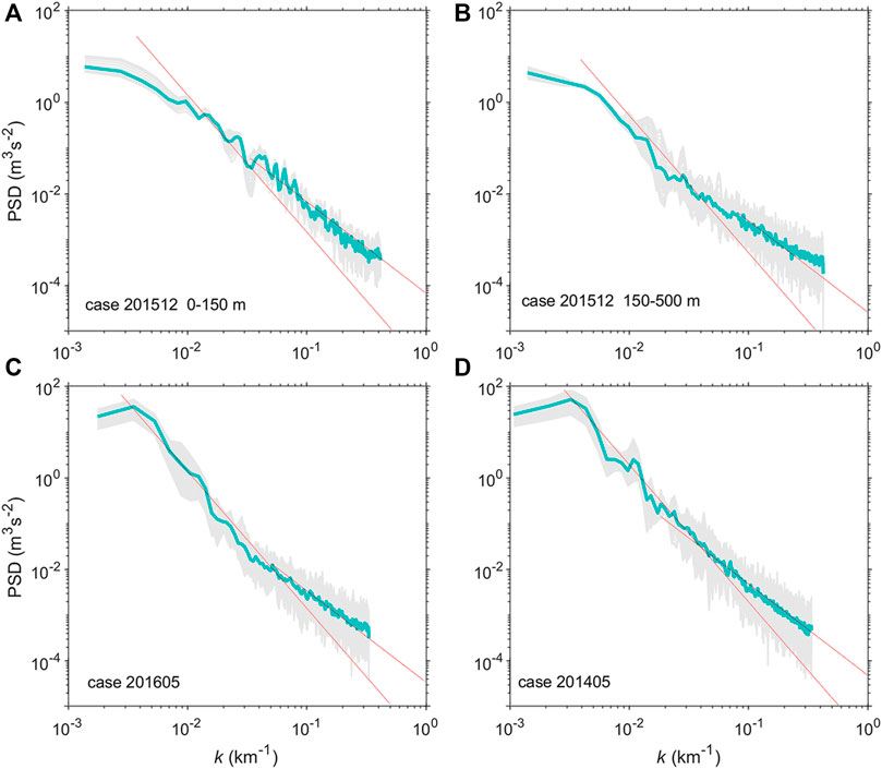
FIGURE 4. Kinetic energy spectra of different cases and different layers. (A) Upper 150 m of case 201512; (B) layer between 150 and 500 m of case 201512; (C) depth average (35–535 m) of case 201605; (D) depth average (35–540 m) of case 201405. The velocities west of 70°W are used to calculate the spectra to exclude the influence of the Gulf Stream. The light gray curves are original spectra at every depth, the green curves denote the averaged states, and the red lines are references of k⁻³ and k⁻².

Besides, the variation of SKE also supports this point. The spatial patterns of SKE of two cases (Figure 5) are similar to their Ro patterns (Figure 2). In case 201512, SKE is intensively elevated in upper 125 m, where there exist plenty of narrow patches with SKE values exceeding O (10⁻³) m² s⁻² while the background value is 10⁻⁴ m² s⁻². The elevated SKE patches in 150 m deeper are significantly scarce when compared with those in the upper 150 m, which are mainly located near 71°W, generated by the Gulf Stream. As for case 201605, the elevated SKE reaching 500 m is mainly due to the Gulf Stream and mesoscale eddies (black and red dashed boxes in Figure 5B); beyond their influence, the magnitude of SKE is also 10⁻⁴ m² s⁻² with few elevated SKE patches, suggesting the weakness of “traditional” submesoscale motions in summer.

FIGURE 5

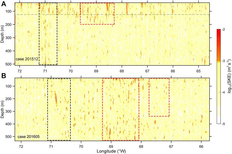
FIGURE 5. Longitude–depth variations of log₁₀(SKE) (m² s⁻²) in case 201512 (A) and case 201605 (B). The gray dashed line marks the mean mixed layer depth 125 m in winter. The black dashed boxes mark the Gulf Stream position, while the red dashed boxes represent the position of mesoscale eddies that generate/influence submesoscale motions.

Discussion

Submesoscale Motions Generated by the Gulf Stream

In both cases of 201512 and 201605, there are distinctly large Ro values extending to 500 m depth near 71°W, with mean Ro value as high as 0.8 (black dashed boxes in Figure 2). Especially in the upper 260 m, the maximum Ro reaches 2.24 and all Ro values are greater than 1. SKE patches exceeding 1 × 10⁻³ m² s⁻² are also common there (black dashed boxes in Figure 5), suggesting the occurrence of a “new type” of submesoscale motion. Compared with the submesoscale motions within the surface mixed layer, these submesoscale motions break the limit of the surface mixed layer and show no clear seasonality.

In combination with sea surface temperature (SST) maps (black dashed boxes in Figures 6A,B) and the velocity magnitude $\left(U=\sqrt{u^2+v^2}\right)$ sections (black dashed boxes in Figures 7A,B) in the same periods, this area is featured with high SST and strong flow. The mean SST in this area is 23°C in winter and 27°C in summer, about 5°C higher than its ambient water; the surface velocity exceeds 2 m s⁻¹ and the velocity at 500 m depth is about 1 m s⁻¹, which are the typical characteristics of the Gulf Stream. The distinctly high temperature and strong velocity peak at the central axis of the Gulf Stream and decrease to its periphery and the outer ambient water, inducing strong lateral gradients of temperature and velocity reaching 0.5°C km⁻¹ and 10⁻⁴ s⁻¹, which fulfill the precondition of frontogenesis and lateral shear instabilities (McWilliams, 2016) and give rise to strong submesoscale motions.

FIGURE 6

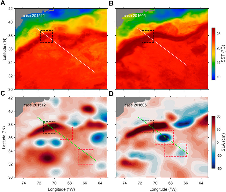
FIGURE 6. Maps of SST (°C) and SLA (cm) of case 201512 (A,C) and case 201605 (B,D). The white lines in (A,B) and the green lines in (C,D) are the vehicle tracks. The black dashed boxes mark the Gulf Stream, and the red dashed boxes mark mesoscale eddies that generate/influence submesoscale motions, consistent with those in Figures 2, 5. The SST data are from the Group for High Resolution Sea Surface Temperature (GHRSST, https://sealevel.nasa.gov/missions/ghrsst), and the sea level anomaly data are produced by SSALTO/DUACS and distributed by AVISO (https://www.aviso.altimetry.fr/en/home.html).

FIGURE 7

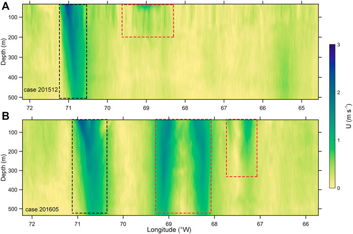
FIGURE 7. Longitude–depth variations of velocity magnitude U (m s⁻¹) in case 201512 (A) and case 201605 (B). The gray dashed line marks the mean mixed layer depth 125 m in winter. The black dashed boxes mark the Gulf Stream position, while the red dashed boxes represent the position of mesoscale eddies that generate/influence submesoscale motions.

Submesoscale Motions Generated by Mesoscale Eddies

Besides the Gulf Stream area, Ro ∼ 0.5 patches and associated elevated SKE patches through the whole upper 500 m are also found between 68.4 and 69.2°W in case 201605 (the middle red dashed box in Figures 2B, 5B). The sea level anomaly (SLA) map (Figure 6D) and velocity magnitude section (Figure 7B) of case 201605 suggest there is a prominent cyclonic mesoscale eddy with a horizontal scale of about 200 km and vertical scale exceeding our deepest measurement (530 m). The rotation of eddy diverges water in the surface, leading to a 60 cm drop of sea surface height (the middle red dashed box in Figure 6D); the deeper colder water moves upward to compensate the loss of water due to the divergence, lowering down the local SST and hence increasing the lateral temperature gradient. Unlike the Gulf Stream, the maximum velocities appear at the periphery of the mesoscale eddy and decrease to both the eddy center and the ambient water (Figure 7B), which results in that the maxima of lateral shear and Ro appear at the periphery of the eddy.

A more convincing case of eddy-driven-submesoscale motions was captured during 8–13 May 2014 (case 201405). Based on the SLA map, the Gulf Stream was temporarily “cut off” by a strong cyclonic eddy (the middle red dashed box in Figure 8E). This eddy is located between 67.3–69.9°W and 35.4–37.8°N with SLA being -80 cm in the eddy center, which intersects with our measurement section between 67.9 and 69.8°W. The intensified flows at the eddy periphery exceed 1 m s⁻¹ throughout our measurements (the middle red dashed box in Figure 8C); especially at the southeast periphery, the velocity maxima reach 2 m s⁻¹ in the whole observed water column. The Ro section shows there are distinct |Ro| patches exceeding 1 at the peripheries of this eddy (the middle red dashed box in Figure 8A). The SKE is also elevated in these areas with large SKE patches exceeding 10⁻³ m² s⁻² (the middle red dashed box in Figure 8B), which is comparable to those energetic submesoscale motions in case 201512.

FIGURE 8

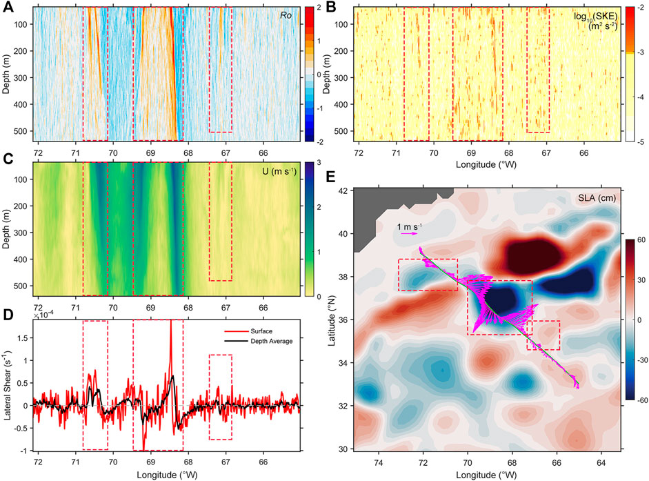
FIGURE 8. Information of case 201405. (A) Section of Rossby number; (B) section of SKE (m² s⁻²); (C) section of velocity magnitude (m s⁻¹); (D) surface and depth-averaged lateral shear (s⁻¹); (E) SLA map (cm) and surface velocity vector (m s⁻¹, magenta arrows); the green curve denotes the section.

The depth-averaged kinetic energy spectra of case 201405 are shown in Figure 4D. Compared with that of case 201512, the spectrum of case 201405 (Figure 4C) follows a k⁻² power law in the wavenumber band ranging from 2 × 10⁻² km⁻¹ to 4 × 10⁻¹ km⁻¹, which is similar to the spectrum in mixed layer (upper 150 m) of case 201512, in which the submesoscale motions are active. Despite that case 201405 and case 201605 are in the same season even the same month, their spectra show distinct slopes, revealing the different active levels of submesoscale motions generated by mesoscale eddies. What should be noticed is this scenario happened in summer, when the surface mixed layer depth is only about 10 m (Figure 3), much thinner and more stable than that in winter, which suggests the submesoscale motions generated by mixed layer instability have neither space nor precondition to sufficiently develop. This implies that the eddy-associated submesoscale motions in deep water in summer are furnished by other processes.

Combining the distributions of large Ro, elevated SKE, and SLA (Figures 8A,B,E), this significant cyclonic eddy is highly correlated with the observed energetic submesoscale motions. As the surface velocity vector along the section (magenta arrows in Figure 8E) suggests, three strong flows exceeding 2 m s⁻¹ are restricted between 67.6 and 70.6°W, which correspond to the Gulf Stream and the intensified flows at the northwest and southeast peripheries of this eddy. Within 375 km from 67.6 to 70.6°W, these flows veer from northeast to southwest and back to northeast, introducing strong lateral shear and vertical vorticity. At the southeast periphery of the eddy, the surface flow reaching 2.35 m s⁻¹ sharply decreases to 0 m s⁻¹ within ∼13 km, which causes extremely strong lateral shear reaching 1.9 × 10⁻⁴ s⁻¹ (red curve in Figure 8D). However, the shear near the eddy center is about 3 × 10⁻⁵ s⁻¹, a magnitude smaller than that of the periphery, which is consistent with the small Ro at the eddy center. The depth-averaged result (black curve in Figure 8D) has relatively small maxima (6 × 10⁻⁵ s⁻¹) but still significantly larger than the eddy central value (1 × 10⁻⁵ s⁻¹). The relative weakness of depth-averaged lateral shear suggests that the lateral shear decreases with the increasing depth, which is similar to the descending Ro from 1.9 at the surface to 0.8 at 400 m. The similarity between Ro and lateral shear suggests that the strong lateral shear should be responsible for the active submesoscale motions at the eddy periphery. Besides, despite the lack of local temperature measurements, the lateral temperature gradient induced by the temperature difference between the inner and outer mesoscale eddies may also contribute to the generation of the submesoscale at the eddy periphery.

Comparing the pattern of Ro, velocity magnitude, and SLA, we can find more examples suggesting mesoscale eddies generate or strengthen submesoscale motions. In case 201512, the Ro ∼ 1 patches near 69°W are deepened to ∼200 m by an anticyclonic eddy in its shedding from the Gulf Stream (the middle red dashed box in Figures 2A, 5A, 6C, 7A). In case 201605, the Ro in the upper 200 m near 67.1 and 67.6°W is elevated by a pair of opposite eddies (the left red dashed box in Figures 2B, 5B, 6D, 7B). In case 201405, the Ro near 67 and 70.5°W is separately elevated by an anticyclonic eddy (the right red dashed box in Figures 8A–E) and a cyclonic eddy (the left red dashed box in Figures 8A–E); the elevation level is correlated with the strength of eddy.

As internal gravity waves may share similar spatial–temporal scales with the submesoscale motions, they cannot be “exactly” distinguished from the submesoscale motions in this study. So, the above analyses of large Ro, elevated SKE, and k⁻² slope spectra could be contaminated if there are internal gravity waves. To exclude the influence of internal waves, a part of section during 2–5 July 2009 (case 200907) is examined (red dashed box in Figure 9A, corresponding to the gray part of section in Figure 9C). As the SLA map (Figure 9C) suggests, this part of section is beyond the influence of mesoscale eddies, and the corresponding Ro is relatively small (Figure 9A), indicating the absence of submesoscale motions. The kinetic energy spectra show no slope of k⁻² but are nearly identical to k⁻³ (Figure 9B), suggesting there are also no internal waves. Combining cases 200907 and 201405, the difference between them is the existence of mesoscale eddies and the submesoscale motions generated by them, and their kinetic energy spectra show distinct slopes. This difference suggests the k⁻² slope of spectra in case 201405 is due to the submesoscale motions. Although the internal wave signal cannot be fully removed, this comparison may exclude the influence of internal waves to some extent.

FIGURE 9

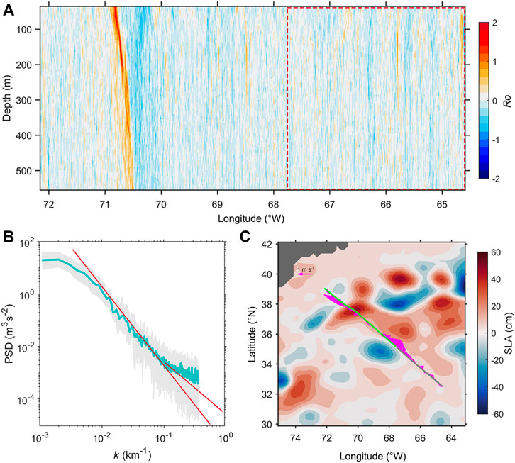
FIGURE 9. Information of case 200907. (A) Section of Rossby number, where the red dashed box marks the part of section being examined; (B) kinetic energy spectra; the light gray curves are original spectra at every depth, the green curves denote the averaged state, and the red lines are references of k⁻³ and k⁻²; (C) SLA map (cm) and surface velocity vector (m s⁻¹, magenta arrows); the green curve denotes the section, and the gray curve is the part being examined.

Conclusion

The high-resolution observational data from the Oleander Project are used to investigate the submesoscale dynamics in the area between New Jersey Shelf and Bermuda. Based on analyses of the vertical variation of Rossby number, kinetic energy in the submesoscale range, and kinetic energy spectra, the results suggest submesoscale motions are active within the mixed layer with seasonality being strong in winter and weak in summer. Besides, submesoscale motions beneath the surface mixed layer are found in summer, some even reaching 500 m depth, and they show no clear seasonality. The large-scale Gulf Stream and mesoscale eddies may be responsible for the following: the strong lateral shear, existing in the Gulf Stream and at the eddy periphery and occupying their entire influence depths, is capable of breaking the geostrophic balance and generating active submesoscale motions beneath the surface mixed layer.

Filaments at the mesoscale eddy periphery are a typical form of submesoscale motions in the sea surface and mixed layer (McWilliams, 2016; Yang et al., 2017). Our result suggests that the lateral shear–induced submesoscale motions in the Gulf Stream and at the eddy periphery can break through the limitations of the surface mixed layer and occur in the ocean interior in summer, in which the lateral shear results from drastically varying flows of the large-scale Gulf Stream and mesoscale eddies.

Data Availability Statement

Publicly available datasets were analyzed in this study. These data can be found here: The datasets analyzed in this study are available in the website of Oleander Project (http://po.msrc.sunysb.edu/Oleander/). Besides, the bathymetry data are taken from ETOPO2 2 min Gridded Global Relief Data (https://ngdc.noaa.gov/mgg/global/etopo2.html), the sea surface velocity data are from ECCO Version 4 release 4 (V4r4, https://ecco-group.org/products-ECCO-V4r4.htm), the sea surface temperature data are from the Group for High Resolution Sea Surface Temperature (GHRSST, https://sealevel.nasa.gov/missions/ghrsst), and the sea level anomaly data are produced by SSALTO/DUACS and distributed by AVISO (https://www.aviso.altimetry.fr/en/home.html).

Author Contributions

JL and XW conceptualized the research idea. JL was involved in formal analysis and original draft preparation. XW reviewed and edited the paper. All authors have read and agreed to the published version of the manuscript.

Funding

This work was jointly supported by the Natural Science Outstanding Youth Fund of Shandong Province (ZR2019JQ13), National Natural Science Foundation of China (42076012 and 42006012), and National Key R&D Program of China (2019YFB1504402).

Conflict of Interest

The authors declare that the research was conducted in the absence of any commercial or financial relationships that could be construed as a potential conflict of interest.

Publisher’s Note

All claims expressed in this article are solely those of the authors and do not necessarily represent those of their affiliated organizations, or those of the publisher, the editors, and the reviewers. Any product that may be evaluated in this article, or claim that may be made by its manufacturer, is not guaranteed or endorsed by the publisher.

Acknowledgments

We thank the Oleander group for collecting and sharing the available long-term ADCP and XBT data.

References

Boccaletti, G., Ferrari, R., and Fox-Kemper, B. (2007). Mixed Layer Instabilities and Restratification. J. Phys. Oceanogr. 37, 2228–2250. doi:10.1175/JPO3101.1

CrossRef Full Text | Google Scholar

Buckingham, C. E., Naveira Garabato, A. C., Thompson, A. F., Brannigan, L., Lazar, A., Marshall, D. P., et al. (2016). Seasonality of Submesoscale Flows in the Ocean Surface Boundary Layer. Geophys. Res. Lett. 43, 2118–2126. doi:10.1002/2016GL068009

CrossRef Full Text | Google Scholar

Callies, J., Ferrari, R., Klymak, J. M., and Gula, J. (2015). Seasonality in Submesoscale Turbulence. Nat. Commun. 6, 6862. doi:10.1038/ncomms7862

PubMed Abstract | CrossRef Full Text | Google Scholar

Callies, J. (2018). Restratification of Abyssal Mixing Layers by Submesoscale Baroclinic Eddies. J. Phys. Oceanogr. 48, 1995–2010. doi:10.1175/JPO-D-18-0082.1

CrossRef Full Text | Google Scholar

Capet, X., McWilliams, J. C., Molemaker, M. J., and Shchepetkin, A. F. (2008). Mesoscale to Submesoscale Transition in the California Current System. Part I: Flow Structure, Eddy Flux, and Observational Tests. J. Phys. Oceanogr. 38, 29–43. doi:10.1175/2007JPO3671.1

CrossRef Full Text | Google Scholar

de Boyer Montégut, C., Madec, G., Fischer, A. S., Lazar, A., and Iudicone, D. (2004). Mixed Layer Depth over the Global Ocean: An Examination of Profile Data and a Profile-Based Climatology. J. Geophys. Res. 109, C12003. doi:10.1029/2004JC002378

CrossRef Full Text | Google Scholar

Flagg, C. N., Schwartze, G., Gottlieb, E., and Rossby, T. (1998). Operating an Acoustic Doppler Current Profiler Aboard a Container Vessel, J. Atmos. Oceanic Technol. 15, 2572–3271. doi:10.1175/1520-0426(1998)015<0257:OAADCP>2.010.1175/1520-0426(1998)015<0257:oaadcp>2.0.co;2

CrossRef Full Text | Google Scholar

Forget, G., Campin, J.-M., Heimbach, P., Hill, C. N., Ponte, R. M., and Wunsch, C. (2015). ECCO Version 4: an Integrated Framework for Non-linear Inverse Modeling and Global Ocean State Estimation. Geosci. Model. Dev. 8, 3071–3104. doi:10.5194/gmd-8-3071-2015

CrossRef Full Text | Google Scholar

Fox-Kemper, B., Ferrari, R., and Hallberg, R. (2008). Parameterization of Mixed Layer Eddies. Part I: Theory and Diagnosis. J. Phys. Oceanogr. 38, 1145–1165. doi:10.1175/2007JPO3792.1

CrossRef Full Text | Google Scholar

Fu, L.-L., Chelton, D., Le Traon, P.-Y., and Morrow, R. (2010). Eddy Dynamics from Satellite Altimetry. Oceanog. 23, 14–25. doi:10.5670/oceanog.2010.02

CrossRef Full Text | Google Scholar

ECCO Consortium Fukumori, I., Wang, O., Fenty, I., Forget, G., Heimbach, P., et al. (2021a). Data from: ECCO Central Estimate (Version 4 Release 4). Moffett Field: NAS ECCO Data Portal. https://data.nas.nasa.gov/ecco/data.php?dir=/eccodata/llc_90/ECCOv4/Release4.

Google Scholar

ECCO Consortium Fukumori, I., Wang, O., Fenty, I., Forget, G., Heimbach, P., et al. (2021b). Synopsis of the ECCO Central Production Global Ocean and Sea-Ice State Estimate. Version 4 Release 4. doi:10.5281/zenodo.4533349

CrossRef Full Text | Google Scholar

Gula, J., Molemaker, M. J., and McWilliams, J. C. (2014). Submesoscale Cold Filaments in the Gulf Stream. J. Phys. Oceanogr. 44, 2617–2643. doi:10.1175/JPO-D-14-0029.1

CrossRef Full Text | Google Scholar

Gula, J., Molemaker, M. J., and McWilliams, J. C. (2015). Topographic Vorticity Generation, Submesoscale Instability and Vortex Street Formation in the Gulf Stream. Geophys. Res. Lett. 42, 4054–4062. doi:10.1002/2015GL063731

CrossRef Full Text | Google Scholar

Klein, P., and Lapeyre, G. (2009). The Oceanic Vertical Pump Induced by Mesoscale and Submesoscale Turbulence. Annu. Rev. Mar. Sci. 1, 351–375. doi:10.1146/annurev.marine.010908.163704

PubMed Abstract | CrossRef Full Text | Google Scholar

Kolmogorov, A. N., Levin, V., Hunt, J. C. R., Phillips, O. M., and Williams, D. (1991). Dissipation of Energy in the Locally Isotropic Turbulence. Proc. R. Soc. Lond. A. 434, 15–17. doi:10.1098/rspa.1991.0076

CrossRef Full Text | Google Scholar

Lapeyre, G., Klein, P., and Hua, B. L. (2006). Oceanic Restratification Forced by Surface Frontogenesis. J. Phys. Oceanogr. 36, 1577–1590. doi:10.1175/JPO2923.1

CrossRef Full Text | Google Scholar

Lévy, M., Klein, P., and Treguier, A.-M. (2001). Impact of Sub-mesoscale Physics on Production and Subduction of Phytoplankton in an Oligotrophic Regime. J. Mar. Res. 59, 535–565. doi:10.1357/002224001762842181

CrossRef Full Text | Google Scholar

Mahadevan, A. (2016). The Impact of Submesoscale Physics on Primary Productivity of Plankton. Annu. Rev. Mar. Sci. 8, 161–184. doi:10.1146/annurev-marine-010814-015912

PubMed Abstract | CrossRef Full Text | Google Scholar

Martin, A. P., and Pondaven, P. (2003). On Estimates for the Vertical Nitrate Flux Due to Eddy Pumping. J. Geophys. Res. 108, 3359. doi:10.1029/2003JC001841

CrossRef Full Text | Google Scholar

McWilliams, J. C. (2016). Submesoscale Currents in the Ocean. Proc. R. Soc. A. 472, 20160117. doi:10.1098/rspa.2016.0117

PubMed Abstract | CrossRef Full Text | Google Scholar

Mensa, J. A., Garraffo, Z., Griffa, A., Özgökmen, T. M., Haza, A., and Veneziani, M. (2013). Seasonality of the Submesoscale Dynamics in the Gulf Stream Region. Ocean Dyn. 63, 923–941. doi:10.1007/s10236-013-0633-1

CrossRef Full Text | Google Scholar

Molemaker, M. J., McWilliams, J. C., and Dewar, W. K. (2015). Submesoscale Instability and Generation of Mesoscale Anticyclones Near a Separation of the California Undercurrent. J. Phys. Oceanogr. 45, 613–629. doi:10.1175/JPO-D-13-0225.1

CrossRef Full Text | Google Scholar

Oschlies, A. (2002). Can Eddies Make Ocean Deserts Bloom? Glob. Biogeochem. Cycles 16, 53–61. doi:10.1029/2001GB001830

CrossRef Full Text | Google Scholar

Oschlies, A. (2008). “Eddies and Upper-Ocean Nutrient Supply,” in Ocean Modeling in an Eddying Regime. Editors M. W. Hecht, and H. Hasumi American Geophysical Union AGU, 115–130. doi:10.1029/177GM09

CrossRef Full Text | Google Scholar

Pollard, R. T., and Regier, L. A. (1992). Vorticity and Vertical Circulation at an Ocean Front, J. Phys. Oceanogr. 22, 6092–6625. doi:10.1175/1520-0485(1992)022<0609:vavcaa>2.0.co;2

CrossRef Full Text | Google Scholar

Qiu, B., Chen, S., Klein, P., Sasaki, H., and Sasai, Y. (2014). Seasonal Mesoscale and Submesoscale Eddy Variability along the North Pacific Subtropical Countercurrent. J. Phys. Oceanogr. 44, 3079–3098. doi:10.1175/JPO-D-14-0071.1

CrossRef Full Text | Google Scholar

Taylor, J. R., and Ferrari, R. (2011). Ocean Fronts Trigger High Latitude Phytoplankton Blooms. Geophys. Res. Lett. 38, a–n. doi:10.1029/2011GL049312

CrossRef Full Text | Google Scholar

Thomas, L. N., Tandon, A., and Mahadevan, A. (2008). “Submesoscale Processes and Dynamics,” in Ocean Modeling in an Eddying Regime. Editors M. W. Hecht, and H. Hasumi American Geophysical Union AGU, 17–38. doi:10.1029/177GM04

CrossRef Full Text | Google Scholar

Wenegrat, J. O., Callies, J., and Thomas, L. N. (2018). Submesoscale Baroclinic Instability in the Bottom Boundary Layer. J. Phys. Oceanogr. 48, 2571–2592. doi:10.1175/JPO-D-17-0264.1

CrossRef Full Text | Google Scholar

Yang, Q., Zhao, W., Liang, X., Dong, J., and Tian, J. (2017). Elevated Mixing in the Periphery of Mesoscale Eddies in the South China Sea. J. Phys. Oceanogr. 47, 895–907. doi:10.1175/JPO-D-16-0256.1

CrossRef Full Text | Google Scholar