
94% of researchers rate our articles as excellent or good
Learn more about the work of our research integrity team to safeguard the quality of each article we publish.
Find out more
ORIGINAL RESEARCH article
Front. Earth Sci., 11 April 2022
Sec. Cryospheric Sciences
Volume 10 - 2022 | https://doi.org/10.3389/feart.2022.848007
This article is part of the Research TopicCryosphere and Climate Change in the Arctic, the Antarctic and the Tibetan PlateauView all 24 articles
 Xia He1,2
 Shiqiao Zhou1,2*
A glacier inventory contains data that are important for understanding the hydrology, water resources, and impacts of climate change in glaciated regions. Ten glacier inventories have been created for the Third Pole Region (TPR) or high-mountain Asia, but they vary largely in spatial coverage area and data quality. Therefore, it is necessary to assess the data quality to help potential users choose the right glacier inventories for their research. Using the analytical hierarchy process, this study selects eight assessment factors and quantifies the quality of eight glacier inventories of the TPR. The eight glacier inventories that we assessed are the Randolph Glacier Inventory (RGI), the Glacier Area Mapping for Discharge in Asian Mountains (GGI18), the Second Chinese Glacier Inventory (CGI-2), the Glacier Inventory of the Hindu Kush–Himalayan Region (HKHGI), the Glacier Inventory for the Western Himalayas (WHGI), the Glacier Inventory for the Karakoram and Pamir Region (KPGI), the Second Glacier Inventory of Pakistan (PGI-2) and the Glacier Inventory for the Southeastern Tibetan Plateau (SETPGI). The assessment results indicate that the overall quality of the small-scale glacier inventories of WHGI, KPGI, PGI-2, and SETPGI is higher than that of the large-scale inventories of RGI, GGI18, CGI-2, and HKHGI. For the large-scale inventories, the quality-ranking order from high to low is CGI-2, GGI18, RGI, and HKHGI. However, the comprehensive quality of CGI-2 and GGI18 is comparable over the area covered by CGI-2. The comprehensive quality of CGI-2, GGI18, and RGI exhibits clear spatial differences. Overall, the data quality is higher for the inner TPR than for the surrounding areas. By merging the products of the eight glacier inventories, a new glacier inventory product of the best comprehensive quality was derived for the entire TPR. This new product resembles the spatial distribution of the best-quality glacier inventories of the regions where the different products overlap. In terms of specific regions, the CGI-2 and GGI18 are the best products for most parts of the TPR in China, except for an area of southeastern Tibet where the highest-quality data are from the SETPGI. The other main distributions of the best products are the WHGI for the western Himalayas, the GGI18 and HKHGI for the Hindu Kush and the middle and eastern Himalayas, the PGI-2 for Pakistan, the KPGI for the Karakorum–Pamir area, and the GGI18 and CGI-2 for the Tianshan Mountains. The new data product greatly promotes the quality of a single glacier inventory for the entire TPR. This database will meet the needs of a variety of potential researchers, including those who prefer to get information for a particular parameter from a single glacier inventory (http://data.tpdc.ac.cn/en/data).
Glaciers are significant solid water resources and are extensively developed in the polar regions and high mountains of the middle and low latitudes. According to the Randolph Glacier Inventory (RGI) Consortium 2017 (RGI Consortium 2017), approximately 215,000 glaciers are distributed in the high-mountain regions around the world. It is critical to study mountain glaciers, as their mass balance and meltwater amount are very sensitive to climate change, and they are often located in close proximity to human residential areas (Immerzeel et al., 2013). Determining the number, area, distribution, and rate of change to glaciers is crucial for the development of regions where sources of water are scarce. Quantifying these glacial parameters, especially for large regions, is generally based on a glacier inventory. A glacier inventory contains standardized information about the attributes of individual glaciers, including longitude, latitude, length, area, elevation, slope, aspect, etc. This information provides a basis for research related to glacier change (Sorg et al., 2012), ice volume estimates (Radić and Hock, 2010; Grinsted, 2013; Bahr et al., 2015; Farinotti et al., 2019), hydrological modeling (Radić and Hock, 2011), regional water resource planning, and prediction of global sea level change (Gardner et al., 2013).
Glacier inventory databases have been established with the development of remote-sensing technology in recent decades (Raup et al., 2007; Sakai, 2019). In the past, glaciers were investigated primarily by field observations or using topographic maps and low-altitude aerial photography (Shi et al., 2009). As most glaciers are distributed in remote regions with harsh climates that are difficult to access, only 1% of global glaciers were regularly monitored before the 1970s (Shi et al., 2009; WGMS, 2021). In recent decades, the accumulation of satellite image data, such as from Landsat (MSS/TM/ETM+), ASTER, SPOT, ALOS PALSAR, and Sentinel-2, has allowed for the development of glacier inventory databases. To date, more than one hundred glacier inventories of different scales have been created by different organizations and individual researchers (Raup et al., 2007; Paul et al., 2009b; Cogley, 2009; Ohmura, 2009; Bajracharya and Shrestha, 2011; Frey et al., 2012; Williams, 2013; Bajracharya et al., 2014; Fischer et al., 2014; Guo et al., 2015; Nuimura et al., 2015; Smiraglia et al., 2015; Ke et al., 2016; Ye et al., 2017; Mölg et al., 2018; Sakai, 2019). These glacier inventories provide vital data for a variety of research objectives (Immerzeel et al., 2010; Nuimura et al., 2012; Huss and Hock, 2015; Dehecq et al., 2019; Naegeli et al., 2019; Shannon et al., 2019). However, these data inventories vary in many aspects, including their spatial coverage, remote-sensing data source, mapping method, interpretation, and intended use (Racoviteanu et al., 2009; Ojha et al., 2017; Paul et al., 2017). These differences raise the question of how to choose an appropriate inventory or product for a specific application. Therefore, it is necessary to assess the quality of glacier inventories to provide information for people to choose the best glacier inventory for their research.
The Third Pole Region (TPR) refers to high Asia (25–45°N, 65–105°E), including the Tibetan Plateau and its surrounding high-altitude areas of the Himalayas, the Hindu Kush, the Pamirs, and the Tianshan Mountains. The TPR corresponds to the regions of Central Asia, South Asia West, and South Asia East in the RGI (Pfeffer et al., 2014). With an average height of more than 3,000 m above sea level, the TPR has a total number of 95,536 glaciers, covering 97,606 km2 (RGI Consortium 2017). In the context of global warming, significant glacier change has occurred in the TPR in recent decades (Bolch et al., 2012; Jacob et al., 2012; Yao et al., 2012; Zemp et al., 2015; Brun et al., 2017). Glacier inventory data are essential to accurately quantify how glaciers are changing. We investigated glacier inventories and found that there are ten available for the TPR (Table 1). These glacier inventories partly or entirely overlap each other in terms of their spatial extent. There are often significant differences in glacier number and area between overlapping inventories. For example, for an area of the Tianshan Mountains (Area A in Figure 1), the Second Chinese Glacier Inventory (CGI-2) gives a total glacier number and area of 160 and 1,219.3 km2, respectively (Guo et al., 2015), while the updated version of the Glacier Area Mapping for Discharge in Asian Mountains (GAMDAM, GGI18) gives values of 191 and 938.9 km2, respectively (Nuimura et al., 2015; Sakai, 2019). Therefore, the data quality of glacier inventories needs to be assessed, and no attempt has been made on this work so far. This study performs a comprehensive assessment of the quality of glacier inventories in the TPR using a multi-factor index method.
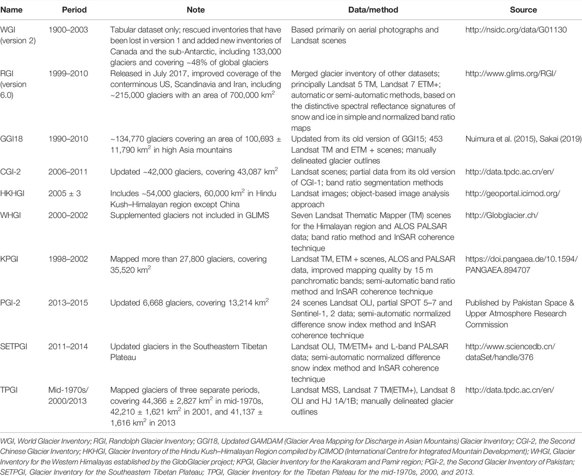
TABLE 1. Key information about the ten glacier inventories for the TPR.
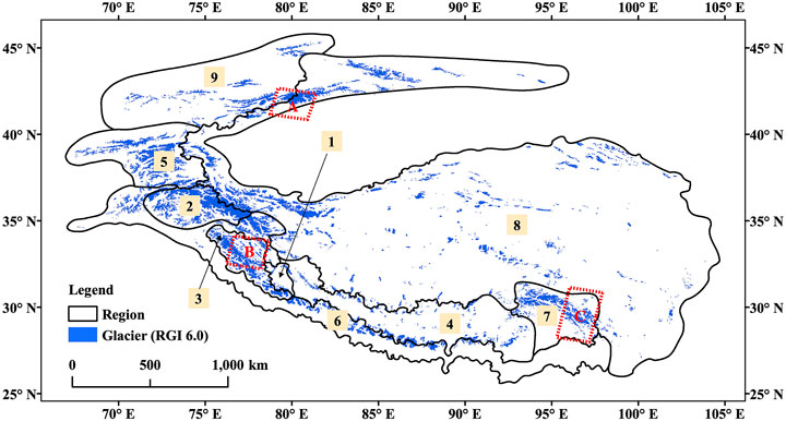
FIGURE 1. Overlap of the glacier inventory products generates nine regions, with each covered by a group of different overlapped products. The three areas with dashed lines, A, B, C are those of overlapped inventories that have a same timestamp for each area. See Table 2 and the text for details.
Among the current ten glacier inventories of the TPR (Table 1), two are hard to assess due to the lack of necessary information. One is the World Glacier Inventory (WGI) (Cogley, 2009), and the other is the Tibetan Plateau glacier data product (TPGI) by Ye et al. (2017). The WGI is a tabular dataset that lacks glacier outlines, and the TPGI is missing the recording dates of remote-sensing images. The following eight inventories were assessed in this study: the RGI (version 6.0); the GGI18; the CGI-2; the Glacier Inventory of the Hindu Kush–Himalayan Region (HKHGI); the Glacier Inventory for the Western Himalayas (WHGI); the Glacier Inventory for the Karakoram and Pamir Region (KPGI); the Second Glacier Inventory of Pakistan (PGI-2); and the Glacier Inventory for the southeastern Tibetan Plateau (SETPGI). Among these inventories, the RGI is somewhat special, as it directly adopts and merges other inventories into one database. As the RGI is a commonly used inventory on a global scale, it is included in this study. Key information about each glacier inventory is listed in Table 1. The eight glacier inventories vary in their spatial extent, and the coverage overlap of their products generates nine regions, with each covered by a group of different overlapping products (Figure 1; Table 2).
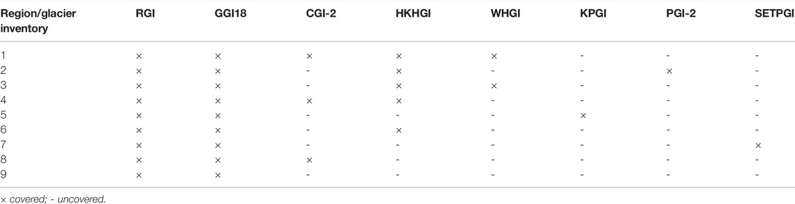
TABLE 2. Spatial coverage of the glacier inventory products, in accordance with the regions where the different products overlap.
Glacier area is the most crucial attribute because it is a fundamental parameter for many research applications. This study identified the primary factors that influence the quality of glacier area data and established a grading index system of these factors based on the analysis of possible error sources in mapping glacier outlines. The weight of each factor was calculated using the analytic hierarchy process (AHP). Using the grading indices and weights of the factors, an assessment value was obtained for each of the assessment units. All of the assessment values were subsequently graded, and the grade of each assessment unit was identified. The assessment unit was determined to be 185 × 185 km2, which corresponds to one scene of a Landsat remote-sensing image.
Data of glacier areas collected in a glacier inventory are primarily obtained from satellite images. According to Paul et al. (2017), this area-obtaining process generally includes four stages: image selection, pre-processing, image interpretation, and post-processing. The assessment factors were screened and selected from the possible error sources involved in these four stages.
The remote-sensing images used by glacier inventories are mainly sourced from Landsat 5, 7, 8, ASTER, IKONOS, SPOT, and ALOS PALSAR. (Pfeffer et al., 2014; Sakai, 2019). Factors related to image selection can be classified into two types: the image resolution and scene conditions of seasonal snow cover, shadows, and cloud cover.
The image resolution directly affects glacier mapping. Generally, outlining the area of glaciers becomes increasingly difficult as the image resolution decreases (Paul et al., 2016). The image resolution was therefore selected as an assessment factor (F1). Seasonal snow cover and shadows, especially those at glacier boundaries, cause uncertainties in the mapping of glacier outlines. These uncertainties, which generally increase with increasing area of snow cover or shadows, are hard to eliminate even in the highest quality images (Bolch et al., 2010; Paul et al., 2011; Paul et al., 2017). Therefore, seasonal snow cover (F2) and shadows (F3) were both selected as assessment factors. A certain distance around the glacier boundary is known as the “buffer zone” and was determined to be 150 m by Guo et al. (2015). The factor of seasonal snow cover was then quantified in terms of the fraction of snow cover in the 150 m wide buffer zone. The factor of shadows is somewhat different, as shadows also cause uncertainties in the inner part of a glacier. The shadow factor was quantified in terms of the fraction of shadow both on the glacier and in the buffer zone. As the cloud cover can be removed by combining scenes from different dates (Paul et al., 2017) or using microwave remote-sensing technology (e.g., synthetic aperture radar (SAR)), this factor was excluded.
The snow cover fraction in the buffer zone at the time of image acquisition was calculated using the daily cloud-free snow product of MODIS in the northern hemisphere (Huang, 2018) from 2000 to 2016. A small portion of the RGI, GGI18, and KPGI was created using remote-sensing images taken prior to 2000, and so, the F2 values for a portion of the data could not be directly calculated due to the lack of snow products. Using MODIS daily data, the data gap of F2 values for the pre-2000 years was filled with the mean F2 values in the same data window of every year from 2000 to 2016. The data window was 9 days and was centered on the pre-2000 imaging day. This data gap filling would not contribute a large error from temporal snow cover changes as the long-term variability of snow cover over the Tibetan Plateau is minimal (Qin et al., 2006; Li et al., 2017).
The shadows, both on the glacier and in the buffer zone, can be obtained from remote-sensing optical data or digital elevation models (DEM). The former method is time-consuming and requires the original remote-sensing data and calculations. Du (2014) compared the two methods and found that the DEM-based method can reduce misinterpretations and is more accurate than the former. This study uses the SRTM (Shuttle Radar Topography Mission) DEM version 4.1, combined with the data about solar altitude angle and azimuth at the time of image acquisition to generate terrain shading images with the ArcGIS Shaded Relief Map (Hillshade).
The pre-processing generally includes radiation calibration and geometric calibration. As these two calibrations had been performed using the same method for all of the satellite images used in glacier inventories, they were excluded in the factor selection. However, the Scan Lines Corrector (SLC) on Landsat 7 experienced a permanent mechanical failure in 2003, and the malfunction caused scan line overlaps, stripes on the image, and a loss of imagery data, which hampers the normal use of the data and brings large uncertainties to glacier area data (Bajracharya and Shrestha, 2011; Paul et al., 2017). Therefore, stripe processing was selected as an assessment factor (F4).
Image interpretation includes the identification and outline mapping of a glacier. During this step, the uncertainties originate mainly from the digitization of debris-covered glaciers. While different glacier mapping methods have little influence on the accuracy of clean glacier outlines (Paul and Kääb, 2005; Paul et al., 2015), the mapping of debris-covered glaciers is more complex, and various methods exist using optical and thermal remote-sensing data. The use of optical data often makes it challenging to differentiate between moraines with and without underlying ice (Paul et al., 2004; Smith et al., 2015). The thermal method is also subject to the limitation of spatial resolution (Alifu et al., 2015; Paul et al., 2015). In recent years, an increasing number of studies have combined optical image classification with Interferometric Synthetic Aperture Radar (InSAR) data (coherence images) to identify debris-covered glaciers (Frey et al., 2012; Ke et al., 2016; Lippl et al., 2018; Mölg et al., 2018). This combination of methods has been reported to be more robust than the optical or thermal remote-sensing methods alone (Brenning et al., 2012; Zbyněk et al., 2012). In addition to the method, the debris-covered extent of a glacier also determines the uncertainty of a measured glacier area. A larger debris-covered fraction of a glacier could lead to a higher uncertainty. Therefore, both the method of glacier outline mapping (F5) and the debris-covered extent of a glacier (F6) were selected as assessment factors. The debris-covered fraction of a glacier was computed using the RGI individual glacier dataset developed by Herreid and Pellicciotti (2020), which was demonstrated to be more accurate than the data from Scherler et al. (2018) (Herreid and Pellicciotti, 2020).
Binary images of glaciers and non-glaciers obtained from automated classification techniques require post-processing to produce the final glacier outlines. The post-processing includes a filtering or morphological opening-and-closing operation, a smoothing process, setting a threshold for the minimum glacier size, quantifying glacier complex segmentation, and manual corrections.
Filtering is primarily used to eliminate small snow patches or fill internal debris and shadow gaps on glaciers. This process has little influence on the ultimate glacier areas (Paul et al., 2017). The process of smoothing sawtooth outlines is performed to improve the aesthetics of glacier boundaries. This is considered to have a very minimal impact on the glacier area due to the minor revisions (Guo et al., 2015). Therefore, both filtering and smoothing were not considered as assessment factors.
After smoothing the glacier outlines, small snow cover patches need to be removed. This process is usually achieved by setting a minimum glacier area threshold and is different for different glacier inventories, generally ranging from 0.01 to 0.05 km2. Setting a larger minimum glacier area threshold (e.g., 0.05 km2) can more likely omit small glaciers, and under good conditions, glaciers of 0.01 km2 can be identified in imagery with 15–30 m resolution (Paul et al., 2009a). Therefore, the minimum glacier area threshold was selected as an assessment factor (F7).
Glacier complex segmentation refers to the segmentation of an acquired glacier complex into individual glaciers. This process does not impact the total glacier area, although it may influence the glacier number. This was not considered as an assessment factor.
The manual correction primarily corrects incorrectly identified snow/shadows and the boundary of debris-covered glaciers (Racoviteanu et al., 2009). This correction is influenced by data features and the personal expertise and judgment of researchers (Andreassen et al., 2008; Paul et al., 2013; Guo et al., 2015; Romshoo et al., 2021). As personal expertise is complex and hard to quantify, only the data features were considered. Of the data features, the glacier size is considered to be a key factor affecting the manual correction, as the larger the size of the glacier, the less the area uncertainty is (Paul et al., 2013; Nagai et al., 2016; Romshoo et al., 2021). Therefore, the manual correction related to the glacier size was selected as an assessment factor (F8).
Glacier size was indexed in relation to the glacier area uncertainty. Paul et al. (2013) investigated the differences of glacier area quantified by different researchers by measuring the same glaciers of different sizes using the same images and under the same conditions. They found that the relative area difference of a glacier tends to be smaller with increasing glacier size. The relative standard deviations are <5% for glaciers larger than 1 km2 and 1%–15% for smaller glaciers. Based on these data, it is assumed that the uncertainty of area for glaciers larger than 1 km2 is one-third of that for smaller glaciers. Following this, the relative uncertainty of area of an assessment unit is determined in terms of the sum of the weighted areal ratios for glaciers both larger and smaller than or equal to 1 km2, which equals (a+(1/3)*(1-a)), where a is the areal ratio of glaciers smaller than or equal to 1 km2 in an assessment unit.
Eight assessment factors were determined using the screening and selection process described above (Table 3). The eight factors were divided into two groups. One group contained the quantifiable factors F2, F3, F6, and F8, whose values were directly normalized to 0–100. The other group contained the factors F1, F4, F5, and F7, which could not be quantified or whose values are discontinuous. These factors were then classified into 2–4 categories, and each category was assigned an index value (Table 3).
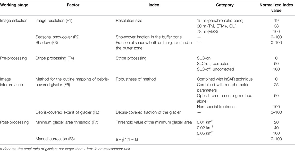
TABLE 3. Assessment factors and their indexes.
The weight for each factor was calculated using the analytic hierarchy process (AHP), which is a multi-criteria decision-making technique developed to analyze complex problems by combining qualitative and quantitative analysis (Saaty, 1990). The AHP enables people to make the most appropriate decision from various criteria by mathematically estimating the relative importance of factors to an event through pairwise comparison and expert judgment. Pairwise comparison of factors allows for the assessment of the significance of a contributing factor compared with other factors and determines the value for each of these factors. A pairwise comparison matrix is generated by assigning a value of 1–9 to each pairwise comparison. A value of 1 in the pairwise comparison matrix means that both factors are equally important, 3 means moderate importance, 5 means strong importance, 7 means very strong importance over the other, and 9 means that one of the factors is extremely important compared with the other. Values of 2, 4, 6, and 8 express intermediate importance values on a scale of 1–9.
The pairwise comparison matrix of this study is shown in Table 4 and was derived based on literature data and expert consultation. In the Glaciers_cci project, Paul et al. (2017) determined that the dominant sources of uncertainty and error for glacier outlines are clouds, seasonal snow, debris cover, and shadow. They found that ice-covered steep mountain flanks might not be included, and glacier extents, including perennial snowfields, can easily be 30% larger or smaller than the data suggests. The potential area differences resulting from interpretations of debris cover can exceed 50% of the total area. On average, a 10%–20% uncertainty for the area of debris-covered glaciers has to be considered (Paul et al., 2017). Nuimura et al. (2015) found a difference of 24% in the total glacier area of high-mountain Asia between GGI15 and RGI and suggested that the difference was probably due to glacial area change, the inclusion or exclusion of shaded glacier areas, seasonal snow cover, and upper steep headwalls. This study also made a comparison between the GGI15 and WHGI and found a glacier area difference of 15% due to differing interpretations of upper steep headwalls. Bolch et al. (2010) estimated an error of ±3% for scenes that have late-lying snow, based on tests where they visually compared automatically derived and manually improved outlines from TM scenes in glacial inventories from western Canada. In the glacier inventory for North Asia, the uncertainty from the manual correction of automatically classified outlines was estimated to be 5.3%, and the uncertainty from image conditions was assigned as 5%, after greatly reducing the effects of image conditions through the manual selection and comparison with Google Earth images (Earl and Gardner, 2016). In Paul et al. (2013), the standard deviation of the difference in the glacier areas of the same glacier derived by different people was 1.6%–30.1% for individual glaciers, with average values of 5.7%, 3.4%, and 3.6% for the three test regions of Alaska, Otztal Alps, and Switzerland, respectively. Using the RGI data from the TPR, glacier areas less than or equal to 0.05 km2 were calculated to be 0.3% of the total glacier area. This value provides a basis for estimating the relative importance of the minimum glacier area threshold factor.
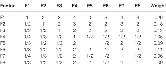
TABLE 4. Pairwise comparison matrix of the factors used in the AHP and the final weights of the factors. See Table 3 for the factors.
The weights of the eight factors were calculated using the pairwise comparison matrix (Table 4) by following the AHP calculations (Saaty, 1990) and are shown in Table 4.
The consistency ratio was calculated based on the eigenvalues of the factors’ matrix to evaluate the consistency of the judgments. A consistency ratio of <0.1 is considered to be acceptable. If the consistency ratio is >0.1, then serious inconsistencies occur, and the AHP may not give meaningful judgments (Prakash and Nagarajan, 2017). The consistency ratio for the comparisons in Table 4 was calculated to be 0.03, indicating good consistency of the judgments.
The weighted index value of each factor for an assessment unit was computed by multiplying the factor weight with the normalized index value. The integrated index value of each assessment unit was then calculated by adding the weighted index values of the eight factors. Figure 2 shows the frequency distributions of the integrated index values for all assessment units of the eight glacier inventories. The frequencies show a roughly normal distribution. According to the characteristics of the frequency distributions, the integrated index values ranging from 29.1 to 51.3 were equidistantly divided into four grades: <36, 36―41, 41―46, and ≧46 for grades 1, 2, 3, and 4, respectively. Grade 1 represents the highest comprehensive quality or lowest uncertainty, while grade 4 represents the lowest quality and highest uncertainty. The cumulative frequencies were then derived to be 18.4%, 39.4%, 30.1%, and 12.1%, respectively, for grades 1, 2, 3, and 4 (Figure 2).
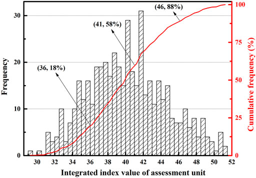
FIGURE 2. Frequency distributions of the integrated index values for all assessment units of the eight glacier inventories.
Figure 3 shows the results of the comprehensive quality assessment for each of the eight glacier inventories. Overall, it is clear that the comprehensive quality of small-scale glacier inventories (WHGI, KPGI, PGI-2, and SETPGI) is generally higher than that of the large-scale glacier inventories (RGI, GGI18, CGI-2, and HKHGI). The small-scale glacier inventories are dominated by grades 1 and 2, except for the PGI-2, where grade 3 makes up a large portion of the data. In contrast, grades 3 and 4 account for a large proportion of the grades in the large-scale glacier inventories. This difference is mainly due to the fact that the small-scale glacier inventories were completed more recently using new satellite data and advanced technology than the large-scale inventories. For example, InSAR data was applied in the development of WHGI, KPGI, and SETPGI (Frey et al., 2012; Ke et al., 2016; Mölg et al., 2018). In addition, the workload of small-scale inventories is much smaller than that of large-scale inventories, which allows for more detailed work.
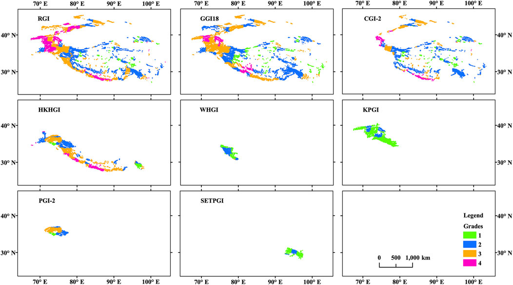
FIGURE 3. Comprehensive quality-grading results of the eight glacier inventories (Grades 1 to 4 represent high to low quality). See Table 1 for the abbreviations.
The quality of the large-scale products of RGI, GGI18, CGI-2 exhibits clear spatial differences. Grades 1 and 2 are mainly distributed in the inner part of the TPR, while grades 3 and 4 are largely on the periphery (Figure 3). Overall, the quality of the glacier inventories of the inner TPR is higher than that of the surrounding areas. This pattern is primarily due to the lower proportion of debris-covered glacier area (Figure 4A) and snow cover (Figure 4B) in the inner TPR. The statistical results of the assessment (Figure 5) indicate that the ranking order of comprehensive quality, from high to low, is CGI-2, GGI18, and RGI. However, it should be noted that the coverage area of the CGI-2 is smaller than that of the GGI18 and RGI (Figure 3). In addition, one portion of the CGI-2 in the southeast Tibetan Plateau (27–31°N, 90–94°E), with a total glacier area of 8,753 km2, is not included in the assessment as it was simply inherited (i.e., not updated) from the CGI-1 and the previous version lacks necessary information such as the imaging date for assessment. For the CGI-2 area of this study, namely all areas in China excluding the area of the southeast Tibetan Plateau mentioned previously, the areal proportion of grades 1–4 is 8.5%, 53.5%, 27.6%, and 10.4%, respectively, for the CGI-2, and 10.1%, 51.1%, 30.8%, and 8.0% for the GGI18. These data indicate the comparable comprehensive quality of these two glacier inventories.
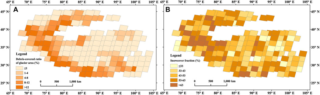
FIGURE 4. The spatial distributions of (A) the debris-covered ratio of glacier area calculated using individual glacier datasets by Herreid and Pellicciotti (2020), (B) snow cover fraction in the buffer zone of a glacier calculated using the GGI18 and the daily cloud-free snow products of MODIS in the northern hemisphere (Huang, 2018) from 2000 to 2016.
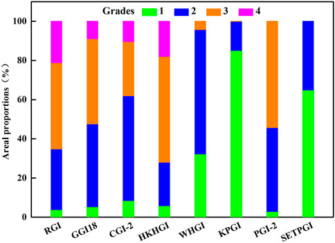
FIGURE 5. Statistical comprehensive quality-grading results of the eight glacier inventories in terms of the areal proportion of the grades.
Table 5 presents the comprehensive quality-grading results of the eight glacier inventories in terms of the nine regions where the different products overlap (Figure 1) and the areal percentages of the different grades for each inventory. Each region is covered by a different group of overlapping glacier inventories, and each glacier inventory is different in the areal percentage of grades, except for the GGI18, the CGI-2, and the RGI in Region 8, where the areal percentages of grades are comparable. The comparable grading results of CGI-2 and RGI are due to the fact that the RGI for this region was almost entirely adopted from the CGI-2. Based on these results, the best-quality glacier inventory for each region was identified (Table 5).
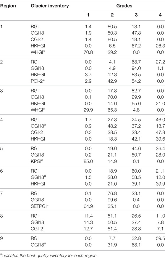
TABLE 5. Comprehensive quality-grading results of the eight glacier inventories for the nine regions of different product overlaps and the areal percentages of grades for each inventory. See Figure 1 for the regions.
A new glacier inventory product of the best comprehensive quality was derived for the entire TPR (Figure 6) by merging products of the eight glacier inventories using the best-quality assessment units or scenes of the overlapped products. This new product largely resembles the spatial distribution of the best-quality glacier inventories of the overlapping regions (Figure 1; Table 5), as most of the best-quality assessment units belong to the best-quality inventories of the regions. The CGI-2 and GGI18 are the best products for most parts of the TPR in China, except for a partial area of southeastern Tibet, where the best is the SETPGI. The other main distributions of the best products are the WHGI for the western Himalayas, the GGI18 and HKHGI for the Hindu Kush, and the middle and eastern Himalayas, the PGI-2 for Pakistan, the KPGI for the Karakorum–Pamir area, and the GGI18 and CGI-2 for the Tianshan Mountains. In the merged product, grades 1 and 2 amount to 74.0% of the total TPR glacier area, which is much higher than the value for the RGI and GGI18 (Figure 5). Grades 3 and 4 only account for 23.8% and 2.2%, respectively, of the total TPR glacier area. A total number of 109,460 glaciers with an area of 101,250 km2 are included in the merged product.
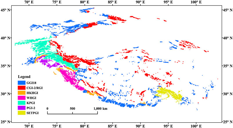
FIGURE 6. A merged glacier inventory product of the best comprehensive quality data from the eight glacier inventories. See text for details.
On the basis of the above work, an open-access database was created (http://data.tpdc.ac.cn/en/data). The database provides the following data: (1) glacier information inherited from the original inventories, including longitude, latitude, length, area, elevation, slope, aspect, and acquisition time of the remote-sensing data; (2) information of the data assessment, including the normalized index values of the eight assessment factors, integrated index values and the grade of scenes for all eight inventories, recorded for individual glaciers. This database will meet the needs of potential users who wish to know the best glacier inventory of comprehensive quality for a specific region or prefer to get information for a particular parameter (e.g., seasonal snow cover) from a single glacier inventory.
The AHP-based approach of glacier inventory assessment is inevitably somewhat subjective, since it is built on a semi-quantitative basis (Prakash and Nagarajan, 2017). In some cases, it is a little difficult to determine the importance of one assessment factor relative to another using pairwise comparison, although substantial literature data were reviewed and expert consultations were conducted. An example is the comparison of the two factors of stripe processing and the minimum glacier area threshold. Nevertheless, these factor pairs are the less important assessment factors, and more data is available for the more important factors.
The cloud cover and/or snow cover removal in glacier inventorying sometimes results in a collage of images with different imaging times for a single scene or assessment unit (Paul et al., 2017). This time difference or time range, which can exceed 10 years (e.g., in GGI18), leads to uncertainty in the glacier area for a specific year due to glacier change (Ye et al., 2017). Strictly, this glacier change should also be selected as an assessment factor, considering that the assessment unit corresponds to the scale of one scene of a Landsat image. However, all glaciers are time-stamped, which excludes the impact of glacier change from the perspective of an individual glacier, and so glacier change was not selected as an assessment factor.
For the factor of seasonal snow cover, the resolution of the applied MODIS product (500 m) may be too low for individual glaciers. However, this resolution is high enough for the assessment unit of 185 × 185 km2 used in this study, and a product of higher resolution is not available at present. A comparison was made to assess the data gap filling of partial snow cover, which is a method that is commonly used in meteorology. The comparison was conducted between the F2 values of assessment units or scenes at the time of image acquisition and those of the same assessment units that used the method of data gap filling. The latter contains the average values from 2000 to 2016, and the former are from post-2000 data, as no pre-2000 data are available. The two datasets are in good agreement (Figure 7). The data gap filling of snow cover is considered to be acceptable as the data gap mainly occurred in 1998–1999, although it does extend back to 1990.
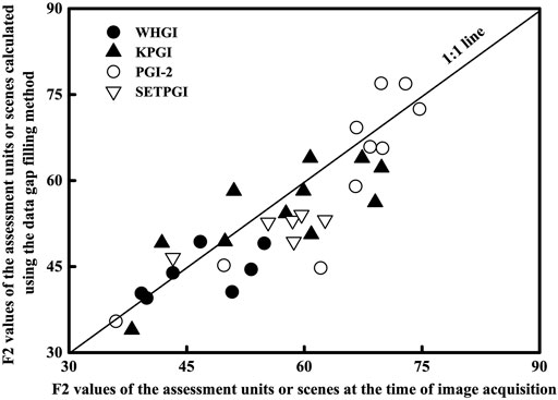
FIGURE 7. Comparison of the F2 values of the assessment units or scenes at the time of image acquisition, with those of the same assessment units calculated using the data gap filling method.
Using the SRTM DEM to calculate shadows might result in an underestimation as the steep mountain ridges causing the shadows are often smoothed in this DEM. However, this underestimation is difficult to determine as the smoothness is unknown.
A lower minimum glacier area threshold is determined to be better and is given a lower index value (Table 3), as it would include more small glaciers. However, a lower threshold might also increase the potential of including more seasonal snow. This uncertainty is hard to estimate, but its impact on the assessment results should be very limited as the weight value for the minimum glacier area threshold factor is only 0.06 (Table 4).
In terms of how the glacier size can affect the manual correction, only a glacier size of 1 km2 is indexed to grading. Other glacier sizes should also have similar effects on the accuracy of the manual correction, although some of the effects (e.g., for sizes larger than 1 km2) could be weaker. However, no data is available for other glacier sizes. In addition, manual correction also depends on snow conditions and the mapping method (Paul et al., 2017). When there is no seasonal snow, and automated mapping is used, small debris-free glaciers (<1 km2) are automatically mapped very precisely, whereas manual mapping tends towards generalization and higher uncertainties. This potential bias is difficult to determine statistically.
All glacier outlines of the GGI18 were manually delineated (Sakai, 2019), while the automated band ratio method combined with manual correction was primarily used in the mapping of other inventories (Pfeffer et al., 2014; Guo et al., 2015; Mölg et al., 2018). Direct comparisons of glacier outlines between the inventories were performed, as this difference between methods is hard to assess due to the uncertain nature of manual work. After screening for all overlapping inventories with the same timestamp, three areas (A, B, C) were identified in the TPR (Figure 1). Information for each of the three areas is listed in Table 6. Not all glaciers in the three areas are included in the table, as not all of them overlap with the same timestamp. A small “snapshot” of overlapping glacier outlines taken from each area is shown in Figure 8. The corresponding false-color (bands 5, 4, 3 as RGB) composite Landsat images and Sentinel-1A InSAR coherence images are also shown in Figure 8 for comparison. Clear differences in glacier outlines can be seen between the overlapping glacier inventories. The outlines for the GGI18 were delineated with more detail compared to those for the CGI-2, RGI, or HKHGI (Figures 8A,B,E,F). Differences in image interpretation are also apparent. Some ice-covered steep headwalls in shadow (Figures 8A,B-1) and part of a debris-covered glacier (Figures 8A,B-2,E,F-2) were not identified in the GGI18, while some bare rocks or seasonal snow cover (Figures 8A,B-3,E/F-3) and moraine (Figures 8A,B-4) were interpreted as a glacier in the CGI-2/RGI/HKHGI. These findings and the data in Table 6 suggest that glacier areas tend to be slightly underestimated for the GGI18 and overestimated for the CGI-2, RGI, or HKHGI, although all of the inventories were identically graded in accordance with the same Landsat images and grading indexes. The glacier outlines of the GGI18 and the WHGI agree relatively well with each other (Figures 8C,D). A clear difference between these inventories is the identification of debris-covered glacier areas (Figures 8C,D-2), where more debris-covered glacier areas were determined in the WHGI due to the use of InSAR data. When looking at data for the entire Area B (Table 6), the most remarkable difference between the two inventories is in the glacier number rather than the glacier area. This large difference in glacier number is due to the different thresholds of minimum glacier area that are used. The minimum glacier area threshold in the GGI18 is 0.01 km2 (Sakai, 2019), and the value in the WHGI is 0.02 km2 (Frey et al., 2012). This threshold difference leads to a larger glacier area in the GGI18 and reduces the gap in glacier area between the two inventories in Area B.
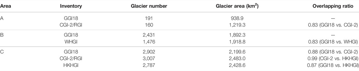
TABLE 6. Comparison of overlapping glacier inventories with the same timestamp for each of the three areas. Note that not all glaciers in the three areas overlap with the same timestamp and only part of the data is included in the table.
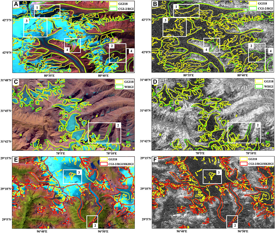
FIGURE 8. Comparison of glacier outlines between overlapping glacier inventories with the same timestamp. The three row pairs are the small “snapshots” of overlapping glacier outlines taken from each of the three areas A, B, C in Figure 1. Also shown are the false-color (bands 5, 4, 3 as RGB) composite Landsat images taken on (A) 24 August 2007, (C) 2 August 2002, (E) 8 September 2005, and the InSAR coherence images created by two Sentinel-1A image pairs taken on (B) 7 June 2015 and 13 July 2015, (D) 13 July 2015 and 18 August 2015, and (F) 25 August 2015 and 18 September 2015. A debris-covered glacier is considered to be well reflected by the dark coherence image. The white rectangles with numbers represent differences in image interpretation related to (1) steep headwall, (2) debris-covered glaciers, (3) bare rock or seasonal snow cover, and (4) moraine. Note that the outlines of both the RGI and the HKHGI completely overlap with those of the CGI-2 due to the fact that their inventory data were directly adopted from the CGI-2 in these areas.
Both precision and the workload of the study were considered when determining the area size of the assessment unit. In general, setting a smaller area size of the assessment unit would lead to more precise assessment results and a larger workload. However, in this study, the situation is somewhat different for a variety of reasons. First, four of the eight assessment factors, F1, F4, F5, and F7, are independent of the area size of the assessment unit, meaning that only the four other factors (F2, F3, F6, and F8) could form more precise result if we used a smaller assessment unit. Second, as data of the four relevant factors are all based on individual glaciers, a differing area size of the assessment unit would only mean a difference in the area size of the statistics. This, being essentially a matter of spatial averaging on different scales, means that even if a smaller area size of assessment unit was applied, the results for the size of 185 × 185 km2 would remain unchanged, although the results for assessment units of a smaller size are more precise. In other words, an F2/F3/F6/F8 value for a larger assessment unit is essentially the average value of all F2/F3/F6/F8 values of the smaller assessment units (i.e., sub-units) within the larger assessment unit.
A sampling analysis was carried out to assess how large this difference could be. Table 7 presents F2 values of the assessment units on two scales for each of the three areas (A, B, C) in Figure 1 using the GGI18 inventory. The two scales are the area sizes of 185 × 185 km2 (UL) and 92.5 × 92.5 km2 (US), meaning that the former contains four of the latter. The differences in the F2 values between UL and US are relatively small, with the largest difference being only 13.7% in Area C2. Therefore, adopting a smaller area size of the assessment unit would result in very limited improvement of precision and no change in the results but cause a much larger workload. On the other hand, the F2/F3/F6/F8 values of some large assessment units can be very precise. This precision is due to the fact that different assessment units of the same area size, such as US or UL in Table 7, contain different glacier areas and numbers. These different glacier areas and numbers lead to variable precisions, as the assessment units with smaller glacier areas and numbers tend to have higher precision due to the statistical nature of downscaling or upscaling. For these reasons, the area size of the assessment unit of 185 × 185 km2 is considered to be suitable and precise enough for the purposes of this study.
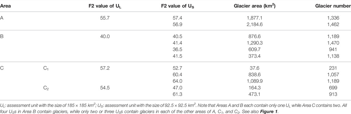
TABLE 7. F2 values of the assessment units on two scales for each of the three areas A, B, and C in Figure 1 using the GGI18 inventory. The corresponding glacier areas and the number of glaciers in each assessment unit are also shown.
Although InSAR technology is used to outline debris-covered glaciers in the TPR, this method has only been applied for small-scale inventories (Table 1). The imaging time is different between InSAR data and the other images used, as the former was developed more recently. This time difference can exceed 10 years (Frey et al., 2012; Mölg et al., 2018) and could introduce uncertainties in final glacier areas due to glacier change. More work is needed to accurately identify debris-covered glaciers in the TPR, potentially by combining GaoFen high-resolution optical data with Sentinel-1A-derived InSAR coherence images.
A comprehensive quality-grading assessment was conducted on eight glacier inventories of the TPR using the AHP method. In general, the comprehensive quality of the small-scale glacier inventories of WHGI, KPGI, PGI-2, and SETPGI is higher than that of the large-scale glacier inventories of RGI, GGI18, CGI-2, and HKHGI. The quality-ranking order from high to low for the large-scale glacier inventories is CGI-2, GGI18, RGI, and HKHGI. The comprehensive quality of the CGI-2 and GGI18 is comparable for the CGI-2 area of this study, as the coverage area of the CGI-2 is smaller, and one portion with relatively low quality is not included due to missing information. The quality of the CGI-2, GGI18, and RGI exhibits clear spatial differences. Overall, their comprehensive quality is higher for the inner TPR than for the surrounding areas. A new glacier inventory product containing the best-quality data was derived for the entire TPR by merging the products of the eight glacier inventories. This new product largely resembles the spatial distribution of the best-quality glacier inventories of inventory-overlapping regions. In terms of specific regions, the CGI-2 and GGI18 are the best products for the majority of glaciers in China, except for a partial area of southeast Tibet, where the best is the SETPGI. The other main distributions of the best products are the WHGI for the western Himalayas, the GGI18 and HKHGI for the Hindu Kush and the middle and eastern Himalayas, the PGI-2 for Pakistan, the KPGI for the Karakorum–Pamir area, and the GGI18 and CGI-2 for the Tianshan Mountains. The new open-access database created in this study greatly increases the quality of a single glacier inventory for the entire TPR and contains full assessment information.
The original contributions presented in the study are included in the article/Supplementary Material (http://data.tpdc.ac.cn/en/data), further inquiries can be directed to the corresponding author.
SZ contributed to conception, design of the study and manuscript. XH performed the analysis. All authors have read and approved the submitted version.
This work was supported by the National Key Research and Development Program of China (Grant No. 2017YFA0603101), the National Natural Science Foundation of China (Grant No. 41771092), the Strategic Priority Research Program of Chinese Academy of Sciences (Grant No. XDA20020102), and the Second Tibetan Plateau Scientific Expedition and Research Program (Grant No. 2019QZKK0202).
The authors declare that the research was conducted in the absence of any commercial or financial relationships that could be construed as a potential conflict of interest.
All claims expressed in this article are solely those of the authors and do not necessarily represent those of their affiliated organizations, or those of the publisher, the editors, and the reviewers. Any product that may be evaluated in this article, or claim that may be made by its manufacturer, is not guaranteed or endorsed by the publisher.
The authors thank Professor Frank Paul for his valuable comments and suggestions, which greatly improved the manuscript. They also thank Professor Yinsheng Zhang for providing the Second Glacier Inventory of Pakistan.
Alifu, H., Tateishi, R., and Johnson, B. (2015). A New Band Ratio Technique for Mapping Debris-Covered Glaciers Using Landsat Imagery and a Digital Elevation Model. Int. J. Remote Sens. 36 (8), 2063–2075. doi:10.1080/2150704x.2015.1034886
Andreassen, L. M., Paul, F., Kääb, A., and Hausberg, J. E. (2008). Landsat-Derived Glacier Inventory for Jotunheimen, Norway, and Deduced Glacier Changes since the 1930s. Cryosphere 2 (3), 131–145. doi:10.5194/tc-2-131-2008
Bahr, D. B., Pfeffer, W. T., and Kaser, G. (2015). A Review of Volume‐Area Scaling of Glaciers. Rev. Geophys. 53 (1), 95–140. doi:10.1002/2014RG000470
Bajracharya, S. R., and Shrestha, B. (2011). The Status of Glaciers in the Hindu Kush-Himalayan Region. Available at: https://lib.icimod.org/record/9419 (Accessed December 22, 2021).doi:10.53055/icimod.551
Bajracharya, S. R., Maharjan, S. B., and Shrestha, F. (2014). The Status and Decadal Change of Glaciers in Bhutan from the 1980s to 2010 Based on Satellite Data. Ann. Glaciol. 55 (66), 159–166. doi:10.3189/2014aog66a125
Bolch, T., Menounos, B., and Wheate, R. (2010). Landsat-based Inventory of Glaciers in Western Canada, 1985-2005. Remote Sens. Environ. 114 (1), 127–137. doi:10.1016/j.rse.2009.08.015
Bolch, T., Kulkarni, A., Kääb, A., Huggel, C., Paul, F., Cogley, J. G., et al. (2012). The State and Fate of Himalayan Glaciers. Science 336 (6079), 310–314. doi:10.1126/science.1215828
Brenning, A., Peña, M. A., Long, S., and Soliman, A. (2012). Thermal Remote Sensing of Ice-Debris Landforms Using ASTER: An Example from the Chilean Andes. Cryosphere 6 (2), 367–382. doi:10.5194/tc-6-367-2012
Brun, F., Berthier, E., Wagnon, P., Kääb, A., and Treichler, D. (2017). A Spatially Resolved Estimate of High Mountain Asia Glacier Mass Balances from 2000 to 2016. Nat. Geosci. 10 (9), 668–673. doi:10.1038/ngeo2999
Cogley, J. G. (2009). A More Complete Version of the World Glacier Inventory. Ann. Glaciol. 50 (53), 32–38. doi:10.3189/172756410790595859
Dehecq, A., Gourmelen, N., Gardner, A. S., Brun, F., Goldberg, D., Nienow, P. W., et al. (2019). Twenty-first century Glacier Slowdown Driven by Mass Loss in High Mountain Asia. Nat. Geosci. 12 (1), 22–27. doi:10.1038/s41561-018-0271-9
Du, W. (2014). Research on Glacier Extraction Based on Multisource RS Imagery and Changes Monitoring of Eastern Tienshan Mountains. Jiaozuo (Henan): Henan Polytechnic University. [doctor’s thesis].
Earl, L., and Gardner, A. (2016). A Satellite-Derived Glacier Inventory for North Asia. Ann. Glaciol. 57 (71), 50–60. doi:10.3189/2016AoG71A008
Farinotti, D., Huss, M., Fürst, J. J., Landmann, J., Machguth, H., Maussion, F., et al. (2019). A Consensus Estimate for the Ice Thickness Distribution of All Glaciers on Earth. Nat. Geosci. 12 (3), 168–173. doi:10.1038/s41561-019-0300-3
Fischer, M., Huss, M., Barboux, C., and Hoelzle, M. (2014). The New Swiss Glacier Inventory SGI2010: Relevance of Using High-Resolution Source Data in Areas Dominated by Very Small Glaciers. Arctic, Antarctic, Alpine Res. 46 (4), 933–945. doi:10.1657/1938-4246-46.4.933
Frey, H., Paul, F., and Strozzi, T. (2012). Compilation of a Glacier Inventory for the Western Himalayas from Satellite Data: Methods, Challenges, and Results. Remote Sens. Environ. 124, 832–843. doi:10.1016/j.rse.2012.06.020
Gardner, A. S., Moholdt, G., Cogley, J. G., Wouters, B., Arendt, A. A., Wahr, J., et al. (2013). A Reconciled Estimate of Glacier Contributions to Sea Level Rise: 2003 to 2009. Science 340 (6134), 852–857. doi:10.1126/science.1234532
Grinsted, A. (2013). An Estimate of Global Glacier Volume. Cryosphere 7 (1), 141–151. doi:10.5194/tc-7-141-2013
Guo, W., Liu, S., Xu, J., Wu, L., Shangguan, D., Yao, X., et al. (2015). The Second Chinese Glacier Inventory: Data, Methods and Results. J. Glaciol. 61 (226), 357–372. doi:10.3189/2015JoG14J209
Herreid, S., and Pellicciotti, F. (2020). The State of Rock Debris Covering Earth's Glaciers. Nat. Geosci. 13 (9), 621–627. doi:10.1038/s41561-020-0615-0
Huang, X. (2018). Data from: Daily Cloud-Free Snow Products of MODIS in the Northern Hemisphere (2000-2016). National Tibetan Plateau Data Center. Available at: http://data.tpdc.ac.cn/en/data (Accessed December 4, 2019).
Huss, M., and Hock, R. (2015). A New Model for Global Glacier Change and Sea-Level Rise. Front. Earth Sci. 3 (54), 54. doi:10.3389/feart.2015.00054
Immerzeel, W. W., van Beek, L. P. H., and Bierkens, M. F. P. (2010). Climate Change Will Affect the Asian Water Towers. Science 328 (5984), 1382–1385. doi:10.1126/science.1183188
Immerzeel, W. W., Pellicciotti, F., and Bierkens, M. F. P. (2013). Rising River Flows throughout the Twenty-First century in Two Himalayan Glacierized Watersheds. Nat. Geosci 6 (9), 742–745. doi:10.1038/ngeo1896
Jacob, T., Wahr, J., Pfeffer, W. T., and Swenson, S. (2012). Recent Contributions of Glaciers and Ice Caps to Sea Level Rise. Nature 482 (7386), 514–518. doi:10.1038/nature10847
Ke, L., Ding, X., Zhang, L., Hu, J., Shum, C. K., and Lu, Z. (2016). Compiling a New Glacier Inventory for southeastern Qinghai-Tibet Plateau from Landsat and PALSAR Data. J. Glaciol. 62 (233), 579–592. doi:10.1017/jog.2016.58
Li, C., Su, F., Yang, D., Tong, K., Meng, F., and Kan, B. (2017). Spatiotemporal Variation of Snow Cover over the Tibetan Plateau Based on MODIS Snow Product, 2001-2014. Int. J. Climatol. 38 (2), 708–728. doi:10.1002/joc.5204
Lippl, S., Vijay, S., and Braun, M. (2018). Automatic Delineation of Debris-Covered Glaciers Using InSAR Coherence Derived from X-, C- and L-Band Radar Data: A Case Study of Yazgyl Glacier. Ann. Glaciol. 64 (27), 811–821. doi:10.1017/jog.2018.70
Mölg, N., Bolch, T., Rastner, P., Strozzi, T., and Paul, F. (2018). A Consistent Glacier Inventory for Karakoram and Pamir Derived from Landsat Data: Distribution of Debris Cover and Mapping Challenges. Earth Syst. Sci. Data 10 (4), 1807–1827. doi:10.5194/essd-10-1807-2018
Naegeli, K., Huss, M., and Hoelzle, M. (2019). Change Detection of Bare-Ice Albedo in the Swiss Alps. Cryosphere 13 (1), 397–412. doi:10.5194/tc-13-397-2019
Nagai, H., Fujita, K., Sakai, A., Nuimura, T., and Tadono, T. (2016). Comparison of Multiple Glacier Inventories with a New Inventory Derived from High-Resolution ALOS Imagery in the Bhutan Himalaya. Cryosphere 10 (1), 65–85. doi:10.5194/tc-10-65-2016
Nuimura, T., Fujita, K., Yamaguchi, S., and Sharma, R. R. (2012). Elevation Changes of Glaciers Revealed by Multitemporal Digital Elevation Models Calibrated by GPS Survey in the Khumbu Region, Nepal Himalaya, 1992-2008. J. Glaciol. 58 (210), 648–656. doi:10.3189/2012jog11j061
Nuimura, T., Sakai, A., Taniguchi, K., Nagai, H., Lamsal, D., Tsutaki, S., et al. (2015). The GAMDAM Glacier Inventory: A Quality-Controlled Inventory of Asian Glaciers. Cryosphere 9 (3), 849–864. doi:10.5194/tc-9-849-2015
Ohmura, A. (2009). Completing the World Glacier Inventory. Ann. Glaciol. 50 (53), 144–148. doi:10.3189/172756410790595840
Ojha, S., Fujita, K., Sakai, A., Nagai, H., and Lamsal, D. (2017). Topographic Controls on the Debris-Cover Extent of Glaciers in the Eastern Himalayas: Regional Analysis Using a Novel High-Resolution Glacier Inventory. Quat. Int. 455, 82–92. doi:10.1016/j.quaint.2017.08.007
Paul, F., and Kääb, A. (2005). Perspectives on the Production of a Glacier Inventory from Multispectral Satellite Data in Arctic Canada: Cumberland Peninsula, Baffin Island. Ann. Glaciol. 42 (1), 59–66. doi:10.3189/172756405781813087
Paul, F., Huggel, C., and Kääb, A. (2004). Combining Satellite Multispectral Image Data and a Digital Elevation Model for Mapping Debris-Covered Glaciers. Remote Sens. Environ. 89 (4), 510–518. doi:10.1016/j.rse.2003.11.007
Paul, F., Barry, R. G., Cogley, J. G., Frey, H., Haeberli, W., Ohmura, A., et al. (2009a). Recommendations for the Compilation of Glacier Inventory Data from Digital Sources. Ann. Glaciol. 50 (53), 119–126. doi:10.3189/172756410790595778
Paul, F., Kääb, A., Rott, H., Shepherd, A., Strozzi, T., and Volden, E. (2009b). GlobGlacier: A New ESA Project to Map the World's Glaciers and Ice Caps from Space. EARSeL eProc. 8 (1), 11–25. doi:10.5167/uzh-29228
Paul, F., Frey, H., and Le Bris, R. (2011). A New Glacier Inventory for the European Alps from Landsat TM Scenes of 2003: Challenges and Results. Ann. Glaciol. 52 (59), 144–152. doi:10.3189/172756411799096295
Paul, F., Barrand, N. E., Baumann, S., Berthier, E., Bolch, T., Casey, K., et al. (2013). On the Accuracy of Glacier Outlines Derived from Remote-Sensing Data. Ann. Glaciol. 54 (63), 171–182. doi:10.3189/2013AoG63A296
Paul, F., Bolch, T., Kääb, A., Nagler, T., Nuth, C., Scharrer, K., et al. (2015). The Glaciers Climate Change Initiative: Methods for Creating Glacier Area, Elevation Change and Velocity Products. Remote Sens. Environ. 162, 408–426. doi:10.1016/j.rse.2013.07.043
Paul, F., Winsvold, S., Kääb, A., Nagler, T., and Schwaizer, G. (2016). Glacier Remote Sensing Using Sentinel-2. Part II: Mapping Glacier Extents and Surface Facies, and Comparison to Landsat 8. Remote Sens. 8 (7), 575. doi:10.3390/rs8070575
Paul, F., Bolch, T., Briggs, K., Kääb, A., McMillan, M., McNabb, R., et al. (2017). Error Sources and Guidelines for Quality Assessment of Glacier Area, Elevation Change, and Velocity Products Derived from Satellite Data in the Glaciers_cci Project. Remote Sens. Environ. 203, 256–275. doi:10.1016/j.rse.2017.08.038
Pfeffer, W. T., Arendt, A. A., Bliss, A., Bolch, T., Cogley, J. G., Gardner, A. S., et al. (2014). The Randolph Glacier Inventory: A Globally Complete Inventory of Glaciers. J. Glaciol. 60 (221), 537–552. doi:10.3189/2014JoG13J176
Prakash, C., and Nagarajan, R. (2017). Outburst Susceptibility Assessment of Moraine-Dammed Lakes in Western Himalaya Using an Analytic Hierarchy Process. Earth Surf. Process. Landforms 42 (14), 2306–2321. doi:10.1002/esp.4185
Qin, D., Liu, S., and Li, P. (2006). Snow Cover Distribution, Variability, and Response to Climate Change in Western China. J. Clim. 19 (9), 1820–1833. doi:10.1175/JCLI3694.1
Racoviteanu, A. E., Paul, F., Raup, B., Khalsa, S. J. S., and Armstrong, R. (2009). Challenges and Recommendations in Mapping of Glacier Parameters from Space: Results of the 2008 Global Land Ice Measurements from Space (GLIMS) Workshop, Boulder, Colorado, USA. Ann. Glaciol. 50 (53), 53–69. doi:10.3189/172756410790595804
Radić, V., and Hock, R. (2010). Regional and Global Volumes of Glaciers Derived from Statistical Upscaling of Glacier Inventory Data. J. Geophys. Res. 115, F01010. doi:10.1029/2009JF001373
Radić, V., and Hock, R. (2011). Regionally Differentiated Contribution of Mountain Glaciers and Ice Caps to Future Sea-Level Rise. Nat. Geosci 4 (2), 91–94. doi:10.1038/ngeo1052
Raup, B., Kääb, A., Kargel, J. S., Bishop, M. P., Hamilton, G., Lee, E., et al. (2007). Remote Sensing and GIS Technology in the Global Land Ice Measurements from Space (GLIMS) Project. Comput. Geosci. 33 (1), 104–125. doi:10.1016/j.cageo.2006.05.015
RGI Consortium (2017). Randolph Glacier Inventory-A Dataset of Global Glacier Outlines: Version 6.0: Technical Report, Global Land Ice Measurements from Space. Colorado, USA: Digital Media. doi:10.7265/N5-RGI-60
Romshoo, S. A., Abdullah, T., and Bhat, M. H. (2021). Evaluation of the Global Glacier Inventories and Assessment of Glacier Elevation Changes over north-western Himalaya. Earth Syst. Sci. Data Discuss.[Preprint]. doi:10.5194/essd-2021-28
Saaty, T. L. (1990). How to Make a Decision: The Analytic Hierarchy Process. Eur. J. Oper. Res. 48 (1), 9–26. doi:10.1016/0377-2217(90)90057-I
Sakai, A. (2019). Brief Communication: Updated GAMDAM Glacier Inventory over High-Mountain Asia. The Cryosphere 13 (7), 2043–2049. doi:10.5194/tc-13-2043-2019
Scherler, D., Wulf, H., and Gorelick, N. (2018). Data from: Supraglacial Debris Cover. Version 1.0. Potsdam, Germany: GFZ Data Services. doi:10.5880/GFZ.3.3.2018.005
Shannon, S., Smith, R., Wiltshire, A., Payne, T., Huss, M., Betts, R., et al. (2019). Global Glacier Volume Projections under High-End Climate Change Scenarios. Cryosphere 13 (1), 325–350. doi:10.5194/tc-13-325-2019
Shi, Y., Liu, C., and Kang, E. (2009). The Glacier Inventory of China. Ann. Glaciol. 50 (53), 1–4. doi:10.3189/172756410790595831
Smiraglia, C., Azzoni, R. S., D'Agata, C., Maragno, D., Fugazza, D., and Diolaiuti, G. A. (2015). The Evolution of the Italian Glaciers from the Previous Data Base to the New Italian Inventory-Preliminary Considerations and Results. Geogr. Fis. Din. Quat. 38 (1), 79–87. doi:10.4461/GFDQ.2015.38.08
Smith, T., Bookhagen, B., and Cannon, F. (2015). Improving Semi-automated Glacier Mapping with a Multi-Method Approach: Applications in central Asia. Cryosphere 9 (5), 1747–1759. doi:10.5194/tc-9-1747-2015
Sorg, A., Bolch, T., Stoffel, M., Solomina, O., and Beniston, M. (2012). Climate Change Impacts on Glaciers and Runoff in Tien Shan (Central Asia). Nat. Clim Change 2 (10), 725–731. doi:10.1038/nclimate1592
WGMS (2021). “Global Glacier Change Bulletin No. 4 (2018-2019),” in ISC(WDS)/IUGG(IACS)/UNEP/UNESCO/WMO. Editors M. Zemp, S. U. Nussbaumer, I. Gärtner-Roer, J. Bannwart, F. Paul, and M. Hoelzle (Zurich, Switzerland: World Glacier Monitoring Service), 278. doi:10.5904/wgms-fog-2021-05
Williams, M. W. (2013). The Status of Glaciers in the Hindu Kush-Himalayan Region. Mountain Res. Dev. 33 (1), 114–115. doi:10.1659/mrd.mm113
Yao, T., Thompson, L., Yang, W., Yu, W., Gao, Y., Guo, X., et al. (2012). Different Glacier Status with Atmospheric Circulations in Tibetan Plateau and Surroundings. Nat. Clim Change 2 (9), 663–667. doi:10.1038/nclimate1580
Ye, Q., Zong, J., Tian, L., Cogley, J. G., Song, C., and Guo, W. (2017). Glacier Changes on the Tibetan Plateau Derived from Landsat Imagery: Mid-1970s - 2000-13. J. Glaciol. 63 (238), 273–287. doi:10.1017/jog.2016.137
Zbyněk, M., Rott, H., Cihlar, J., Schaepman, M. E., García-Santos, G., Fernandes, R., et al. (2012). Sentinels for Science: Potential of Sentinel-1, -2, and -3 Missions for Scientific Observations of Ocean, Cryosphere, and Land. Remote Sens. Environ. 120, 91–101. doi:10.1016/j.rse.2011.09.026
Keywords: Tibetan Plateau, Third Pole Region, glacier inventory, comprehensive quality assessment, high Asia
Citation: He X and Zhou S (2022) An Assessment of Glacier Inventories for the Third Pole Region. Front. Earth Sci. 10:848007. doi: 10.3389/feart.2022.848007
Received: 03 January 2022; Accepted: 03 March 2022;
Published: 11 April 2022.
Edited by:
Minghu Ding, Chinese Academy of Meteorological Sciences, ChinaReviewed by:
Chunhai Xu, Northwest Institute of Eco-Environment and Resources (CAS), ChinaCopyright © 2022 He and Zhou. This is an open-access article distributed under the terms of the Creative Commons Attribution License (CC BY). The use, distribution or reproduction in other forums is permitted, provided the original author(s) and the copyright owner(s) are credited and that the original publication in this journal is cited, in accordance with accepted academic practice. No use, distribution or reproduction is permitted which does not comply with these terms.
*Correspondence: Shiqiao Zhou, emhvdXNocUBpdHBjYXMuYWMuY24=
Disclaimer: All claims expressed in this article are solely those of the authors and do not necessarily represent those of their affiliated organizations, or those of the publisher, the editors and the reviewers. Any product that may be evaluated in this article or claim that may be made by its manufacturer is not guaranteed or endorsed by the publisher.
Research integrity at Frontiers
Learn more about the work of our research integrity team to safeguard the quality of each article we publish.