Earthquake Forecast as a Machine Learning Problem for Imbalanced Datasets: Example of Georgia, Caucasus

1 Introduction

In this article (Chelidze et al., 2020), we considered the problem of earthquake (EQ) forecast using a machine learning (ML) approach, namely, the package ADAM (Kingma and Ba 2014), based on experimental (training) data on monitoring water-level variations in deep wells as well as geomagnetic and tidal time series in Georgia (Caucasus). In the 2020 article, we used the low EQ threshold value of magnitude $M\ge 3$ as a forecast object. In this case, the number of days with EQs of magnitude larger than 3 is less, but of the same order as the number of “aseismic” days, and forecast for EQs of $M\ge 3$ can be considered as the problem of the so-called slightly imbalanced sets; namely, the ratio of “seismic” to “aseismic” days in Georgia is approximately 1:5 for this magnitude range. The forecast problem is actually for stronger EQs, which can cause real damage, as small EQs are not dangerous. When we put the problem of the forecast in this way, the learning datasets became more imbalanced and, for example, the ratio of seismic to aseismic days for in Georgia reaches values between 1:18 and 1:26, which means that the effect of imbalance should be taken into account.

In this article, we apply the ML methodology taking into account the larger magnitude threshold and stronger imbalance in the data.

2 Methodology

2.1 Complexity Analysis and Machine Learning in the Earthquake Forecast

Last decades, using modern methods of complexity analysis allows us to reveal the existence of long-term correlations in the spatial, temporal, and energy distributions in dynamical systems such as seismicity, namely, these distributions in all three domains follow power law (Chelidze et al., 2018). As a result, hidden non-linear structures were discovered in seismic data. These characteristics vary with time, which is in contradiction with the memory-less purely Poissonian approach (Chelidze et al., 2020). The analysis of temporal variations in the complexity of seismic measures, namely, the phase space portrait, can be used for forecasting strong earthquakes (Chelidze et al., 2018).

On the other hand, during last years, the application of machine learning (ML) gained increasing attention in the forecasting laboratory and natural earthquakes (Rouet-Leduc et al., 2017; Rouet-Leduc et al., 2018; Ren et al., 2020; Johnson et al., 2021). By the way, one of the first publications devoted to ML for the EQ forecast belongs to Chelidze et al. (1995), where the generalized portrait method (now support vector machine, SVM) (Vapnik and Chervonenkis, 1974; Vapnik, 1984) was applied to forecast the EQs of magnitude 5 and more in Caucasus for the 5-y period. As the training set, we used the regional seismic catalog and several seismological predictors: the density of seismoactive faults, the slope of the magnitude-frequency relation, the seismic activity rate (the number of events $N$ per unit time), and the emitted seismic energy. As a result, it was shown that the application of the generalized portrait technique using the slope of magnitude-frequency relation $\gamma$ as a predictor allows forecasting retrospectively 85% of 5-y periods with expected M5 events and 100% of calm periods without strong events in Caucasus (Chelidze et al., 1995; Zavjalov, 2006). The addition of a less informative predictor—emitted seismic energy—spoils the total forecast accuracy by 11%.

2.2 The Basic of ML Metrics for Forecasting

One of the main directions of ML is concerned with algorithms designed to accomplish a certain task (forecasting), whose performance improves with the input of more data (Mitchell 1997; Witten et al., 2017; Brunton and Kutz 2020; Brownlee 2021). ML implies that we get information on the future behavior of the system analyzing the data obtained from previous observations after the application of special statistical tools, namely, regression or classification approach. The ML is often used in such diverse fields, such as medicine, geophysics, disaster management, and business (Witten et al., 2017). Applications of ML techniques in the last years have become extremely widespread in solving various problems of seismology, from signal recognition and analysis to forecasting future acoustic/seismic activity on the laboratory and regional scales (Rouet-Leduc et al., 2017; Rouet-Leduc et al., 2018; Chelidze et al., 2020; Ren et al., 2020; Johnson et al., 2021). In our analysis, we consider the problem of forecasting EQs in a given magnitude range and a given time interval using a supervised classification approach, namely, forecasting the probability of occurrence/absence of the seismic event using a previous day geophysical observations’ training dataset. For the analysis of observed data, we used the algorithm of deep learning ADAM (Kingma and Ba, 2014), which optimizes the target function by the combination of the optimization algorithm designed for neural networks (Karpathy, 2017) and a method of stochastic gradient descent with momentum (Bottou and Bousquet 2012).

The classification model forecasts the class of each dataset; as a result, every sample is attributed to one of the following four classes: correctly predicted positives are called true positives (TP), wrongly predicted negatives are called false negatives (FN), correctly predicted negatives are called true negatives (TN), and wrongly predicted positives are called false positives (FP).

2.3 Moderate and Strong EQ Are Rare Events: The Corresponding Forecast Model Is ML on the Imbalanced Datasets

The majority of ML applications are designed for the analysis of the balanced datasets. In the bivariate case, we have two sets of samples: one of them contains the class of events we are interested in and another contains “void” samples without events. When the numbers of each class representatives are about equal, the dataset is considered as a balanced one. At the same time in many cases, the real-world datasets are imbalanced, and we have majority and minority classes; this means that without applying special algorithms, our classification will be biased toward the majority class, and sometimes, the minority class is ignored at all. Such imbalanced classification poses a problem, as quite often just the minority class is of the major interest—say, in disaster forecast, medical diagnostic, business, etc. (Mena and Gonzales, 2006; Malik and Ozturk, 2020). Some widely used classifiers, such as accuracy, are useless if the data are imbalanced. To assess the accuracy classifier, one needs to consider its formulation using the confusion matrix [Chicco and Jurman (2020)], namely, taking into account that accuracy is the total number of correct predictions divided by the total number of predictions:

$\mathrm{Accuracy}=\frac{TP+TN}{TP+FP+TN+FN}.(1)$

It is clear that if the term $TN$ is much larger than $TP$, $FP$, and $FN$, the accuracy can be very high, which is due to high TN values: if $TN$ >> $TN$, $TP$, $FN$, and $FP$, the expression (1) is always close to 100%, which demonstrates that accuracy is not the appropriate classifier for imbalanced data. The imbalance should also be taken into account when using such popular metric as receiver operating characteristic (ROC).

In the seismically active region, such as Georgia, choosing as the forecast object events of larger magnitudes with longer time intervals leads to an increasing imbalance between “seismic” and “aseismic” days. In Georgia, for example, in 2020, the imbalance for events of $M\ge 3.5$ is of the order of 1:20. The imbalances in the range M>6–M<7 and M>7 for the last century increase correspondingly between 1:12250 and 1:36500.

In the present article, we do not use the weak seismic event as precursors of strong EQs, restricting ourselves by other predictor data—hydrodynamic, geomagnetic, and tidal variations.

2.4 EQ Forecast in the Laboratory and in Numerical Models

The stick-slip process, especially under weak periodic forcing, reveals a quite regular pattern in the time domain, if even in the natural stick-slip process, the distribution of waiting times $T_w$ centers on the most probable value, the distribution became much more narrow under weak periodic forcing (Chelidze and Matcharashvili, 2015). Predicting not a statistical distribution of events but the time and amplitude of the next event is much more difficult. New studies show that ML allows prediction of waiting time $T_w$ and amplitude A of the next spike (slip) for laboratory earthquakes more or less exactly having the long enough recording of the previous slip history. Rouet-Leduc et al. (2017, 2018) and Johnson et al. (2021) used the ML random forest algorithm for the analysis of 80 statistical features of acoustic signals before slips (mean value of signal, its variation around mean, etc.) in order to find the time left before the next failure. According to Ren et al. (2020); Johnson et al. (2021), ML can help to resolve the problem, using different AI methods at least for laboratory EQs as well as for specific models of seismicity (namely, cascade or preslip models), where the strong EQs occur after some premonitory aseismic slip (Rouet-Leduc et al., 2018; Ren et al., 2020).

3 Networks, Devices, and Data

The most systematic work oriented to regional short- and middle-term forecast studies in Georgia is connected with a regular monitoring of the water level (WL) in the network of deep wells, operated by the M. Nodia Institute of Geophysics, which began in 1988. Moreover, we analyzed geomagnetic time series recorded by the Dusheti Geophysical Observatory. In the previous work (Chelidze et al., 2020), we analyzed the precursory data of the water level and geomagnetic field variations collected one day before events of magnitudes $M\ge 3.5$ in 2017–2019 on the territory of Georgia. Here, we present the results of the next-day forecast using multiparametric (hydrodynamic, magnetic, and tidal) monitoring data collected one day before events of magnitude $M\ge 3.5$ carried out in 2020 on the territory of Georgia.

The WL monitoring network in Georgia includes several deep wells, drilled in a confined sub-artesian aquifer (Figure 1)—here, we use the data of the five stations with the most systematic records (Table 1). The sampling rate at all these wells is 1/min. Measurements are carried out by sensors MPX5010 with resolution 1% of the scale (company: Freescale Semiconductor; www.freescale.com) and recorded by the XR5 SE-M Data Logger (company: Pace Scientific; http://www.pace-sci.com/data-loggers-xr5.htm). The data are transmitted remotely by the modem, Siemens MC-35i Terminal (company Siemens) using program LogXR. The data logger can acquire WL data for 30 days at the 1/min sampling rate. Variations of the water level represent an integrated response of the aquifer to different periodic and quasiperiodic (tidal variation and atmosphere pressure) as well as to non-periodic influences, including the generation of earthquake-related strains in the earth crust of the order of 0.1–0.001 microstrain. The atmosphere pressure factor was subtracted from the summary WL variations. Magnetic variations were recorded at Dusheti Geophysical Observatory (Lat 42.052°N, Lon 44.42°E), by the fluxgate magnetometer FGE-95 (Japan), registering x, y, and z components at a count rate of 1/sec with accuracy 0.1 nT. The data are representative for a whole territory of Georgia. All these field data present the so-called ground truth, that is, the information obtained on the site, which is used as reality check for the used ML analysis.

FIGURE 1

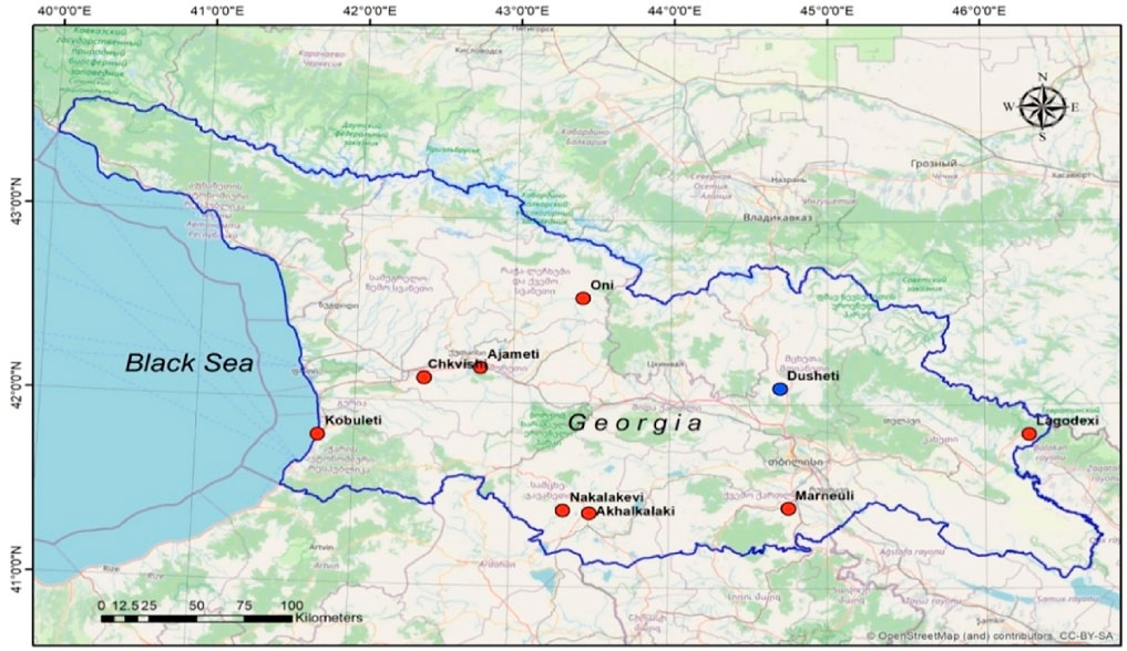
FIGURE 1. Map of Georgia with the location of deep wells’ network (red circles) for water-level monitoring and Dusheti Geomagnetic Observatory (blue circle).

TABLE 1

TABLE 1. Locations and depths of wells in Georgia.

We are looking for hydraulic (Wang and Manga, 2010) and geomagnetic anomalies (Zotov et al., 2013; Buchachenko, 2021) in the “quasiepicentral” or a precursor interaction area R. We choose the interaction length R = 200 km for hydraulic precursors of EQs of $M\ge 3.5$ for a given well. Note that there are different assessments of the EQ precursors’ area. According to the widely used static strain model (Dobrovolsky et al., 1979), the radius R of the anomalous precursory “static” strain area is of the order of 20–30 km for EQs of M3 and 50–70 km for M4. In the “dynamic strain” model (Pregean and Hill, 2009), seismic waves of an initial EQ (source) triggers (induce) secondary seismic events at different distances from the source from meters to thousands of km and with different delays due to dynamic stress perturbations. This approach actually does not restrict the interaction length and the delay range for the inducing event of the hydraulic precursor. We presume that there are at least two physical mechanisms, which can explain the accepted long radius of action of hydraulic precursors (R = 200 km): 1) long-range fluid diffusion from the stressed formation to the well due to poroelastic effects and 2) fast squirt-flow (Dvorkin et al., 1994) of pore water from the impending EQ source to the well, excited by the foreshocks of the imminent event—such signals can travel a long distance (Chelidze et al., 2019).

At the same time, we did not restrict the interaction length at all for geomagnetic precursors. In practice, this means that we accept R for geomagnetic data of the order of 300 km (this is the distance from Dusheti observatory to the most remote well).

4 Results

4.1 Training and Test Datasets

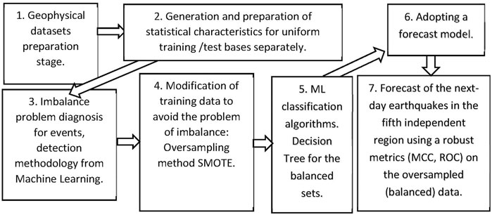
The sequence of actions during machine learning is presented in Figure 2. The first four stages illustrate the process of collection and preliminary processing of training/testing data, and the following three stages show the machine learning process.

FIGURE 2

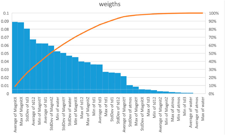
FIGURE 2. Weights of different statistical measures obtained in the process of machine learning using average input data for all five regions (blue columns). The red curve shows the cumulative percent of separate weights.

4.1.1 Geophysical Datasets Preparation Stage

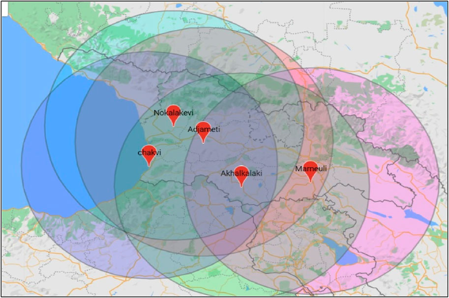
In this article, we consider the statistical values (mean, mean standard deviation, minimal and maximal values, etc.) of the input data—the daily time series of geophysical data (attributes/features), namely, the input data were as follows: water level in the network of boreholes, tidal variations, geomagnetic field intensity, and atmospheric pressure in five circular (overlapping) regions of Georgia centered on the following borehole locations: Ajameti, Akhalkalaki, Kobuleti, Marneuli, and Nokalakevi during 2020 (see Figure 3). We compare these daily values with the data of daily occurrence of EQs of magnitude $M\ge 3.5$ using the machine learning (ML) classification approach (Chelidze et al., 2020): to the days with events of $M\ge 3.5$, we assign value one and to “quiet” days, value 0.

FIGURE 3

FIGURE 3. Map of five separate circular regions around wells with water-level stations.

4.1.2 Generation and Preparation of Statistical Characteristics for Training/Test Bases Separately

As a result, we obtain 32 inputs/attributes—the values of monitoring data for a given day (namely, the day, before the seismic event), and one output with two possible values for the next day—the occurrence (one) or absence (zero) of EQ. For each region, we obtained the table of dimension 33 × 365, where the 33-th column is the target EQ column—that is, the information on occurrence/absence of events in the 200 km radius from the given well. According to our data, in the output columns of regions, the imbalance values are minimum 1:18.

Analysis of Figure 2 leads to the unexpected result—namely, the machine learning approach assigns the largest EQ predictive weight to geomagnetic data. We would like to note here that the recent research (Zotov et al., 2013) made interesting discovery on the magnetic precursors of EQs. According to their data, big magnetic pulses are followed by increase in the number of relatively weak seismic events with a maximum at the magnitude M = 3.9 a few hours after the onset of magnetic anomaly. Balasis et al. (2011) also observed similarity in the universality in solar flares, magnetic storms, and earthquakes using Tsallis statistical mechanics and suppose that these diverse phenomena have a common physical mechanism. It seems that our data (Figure 2) support the mentioned observations: the geomagnetic field intensity is the leading one in the list of precursors of the next day EQ of $M\ge \mathrm{3.5.}$

4.1.3 The Used Machine Learning Methodology: Imbalance Problem for Seismic Events

Thus, we have separate datasets (tables) for five regions (Figure 4). For training, we decided to cluster four regions’ data (here, Ajameti, Akhalkalaki, Kobuleti, and Marneuli) and use these data as a training set for machine, where the output is the occurrence (one) or absence (zero) in the next day of EQ of magnitude $M\ge 3.5$ in the fifth (target) region (Nokalakevi). As a result, after the application of this procedure to all five regions, we obtained 1,445 records, where statistical values of the previous days’ oversampled geophysical data are collected and the original (not oversampled) information on the occurrence/absence of seismic events in the target region next day.

FIGURE 4

FIGURE 4. Scheme of the used machine learning procedure.

As there is a high imbalance in our data with prevalence of “quiet” days without next day events (zero), we used the recommended random oversampling approach (He and Garcia 2009; Brownlee, 2021), where the rare events—(one)—are duplicated in order to increase the minority class.

4.1.4 Modification of Training Data to Avoid the Problem of Imbalance

Some authors note that oversampling of the initial dataset can cause the overfitting effect (Chawla et al., 2018; Brownlee, 2021). In order to avoid the overfitting effect, we integrate the database, obtained in the mentioned four regions and considered it as a joint training base. The fifth region was considered as a testing object, which contains zero or one event, as well as the statistical parameters (precursors) obtained on the previous day.

According to this scheme, after finishing machine learning, the ROC for the testing region was compiled; this shows if the model is adequate for learning on the integrated predicting base of four regions instead of the separated data for a given region. In other words, we trained the model on the four different regions and applied it to the fifth testing region. The aforementioned procedure was carried out for all the possible combinations of four training and fifth testing regions. Finally, we carried out five tests and revealed that resulting ROC diagnostics results are quite close to each other. We presume that due to this procedure, the overfitting effect in all five regions is less probable.

During integration, we used the Python library, namely, the recipe “imblearn.over_sampling” and obtained a new training database with 2,792 artificially replicated ensemble of “seismic” days (due to replicated—added—1 values) with unchanged statistics of “zero” days.

Based on the training ML experience obtained on the ensemble of four regions, we applied to the fifth one here—Nokalakevi, where we tried to forecast EQs, occurred in the target region using the original (non-oversampled) testing part of seismic catalog. Actually, we apply the experience, obtained by training on the four regions’ oversampled data, to a new region in order to carry out the model verification on the original (testing) seismic data for the Nokalakevi region, where 14 EQs of M $\ge$ 3.5 occur in 2020.

4.2 ML Algorithms

4.2.1 Decision Tree and SVM for the Balanced (Oversampled) Sets

As a forecasting method, we used decision tree (DT)—a supervised machine learning algorithm, applied in both classification and regression problems. The DT is preferable because 1) it does not need special pretreatment of data, such as data normalization, addition, or exclusion of data, and special equipment for handling big data; 2) DT allows assessing the reliability of the model using statistical tests. We used the following library: imblearn.over_sampling import SMOTE in Python (Fernández et al., 2018) in order to transform our imbalanced dataset into a balanced one. We illustrate below graphically how the input dataset change after application of this approach; Figure 5A presents the initial imbalanced dataset, where orange points are events (one) and blue points correspond to the quiet state (zero). After the application of SMOTE, the previous graph transforms to Figure 5B, where the dataset became a balanced one.

FIGURE 5

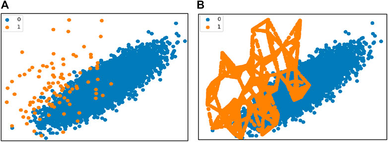
FIGURE 5. (A, B) Graph of the data point distribution (A) presents the initial imbalanced dataset, where orange points are events (one) and blue points correspond to the quiet state (zero); (B) after the application of SMOTE the previous graph transforms to a balanced one.

Finally, our ML workflow for five regions—objects for forecast—is as follows (see also Figure 4).

1) The training data for the chosen four regions are collated and the fifth—testing region with its EQs—is left for further training.

2) The same procedure is repeated for all other five combinations of training and testing regions.

3) As a result, we get five training tables with the following dimensions: 1,464 readings in columns with data (total 33 columns, including the 33rd column for the output—EQ).

4a) The same dimensions have the data in the target (fifth) region. The three training parameters in Python are as follows: X_train, X_test, y_train, y_test = train_test_split(X, y, test_size = 0.3, and random_state = 1) # 70% training and 30% tests.

4b) We also made an attempt to use other training version: clf = DecisionTreeClassifier(criterion = “entropy”, max_depth = 3) for different depths and found that the max_depth = 3 version was optimal, but for all five models the results were slightly worse than for the standard 4a model parameters. In addition, when we are using entropy parameter, the results for different regions were non-stable, so we preferred version 4a.

After dividing the data into training and testing sets, the forecast was carried out and the corresponding five models were compiled.

In order to assess the confidence interval of the trained model for the Akhalkalaki region (with presumption that classification accuracy/error is distributed according to the Gauss model), the following code was used:

Code (95%): from statsmodels.stats.proportion import proportion_confint

lower, upper = proportion_confint(360, 365, 0.05)

print('lower = %.3f, upper = %.3f' % (lower, upper))

lower = 0.974, upper = 0.998

Naturally, the confidence interval depends on accuracy. Here, we remind that our bases are sufficiently imbalanced and zero value—the marker of “no-EQ” event—and lead to almost 100% of confidence interval’s upper and lower values. Note that from 365 days’ records for the Akhalkalaki region, only 20 days contain EQs and our program recognizes 17 of them. If we consider the confidence interval of recognition for EQ events (ones), we obtain for the confidence interval (of course, this method is better to use when the number of events n is > 30).

lower, upper = proportion_confint(17, 20, 0.05)

lower = 0.694, upper = 1.000

Correspondingly, the confidence intervals’ values for other four regions are in the same range.

After transforming the imbalanced datasets into balanced ones, we used the program tree.DecisionTreeClassifier (Pedregosa et al., 2011; Brownlee 2021). Taking into account the stochastic nature of the algorithm and the type of data, we decided that for testing the algorithm and assessing its reliability, it is reasonable to repeat the learning procedure several times and to analyze the resulting confusion matrixes and averaged ROC AUC values.

We choose the algorithm “sklearn” for ML from the library “DecisionTreeClassifier” of Python Scikit-learn package (Pedregosa et al., 2011; Brownlee, 2021) in order to test its EQ forecasting potential on the original (not oversampled) testing data in the fifth—Nokalakevi—region. The results of testing, which we present as the confusion matrix and the receiver operating classification (ROC) graph (Figure 6), show that the applied methodology leads to quite satisfactory result: according to the confusion matrix, ML success cases amount to 12 from total 14 events with two false forecasts.

FIGURE 6

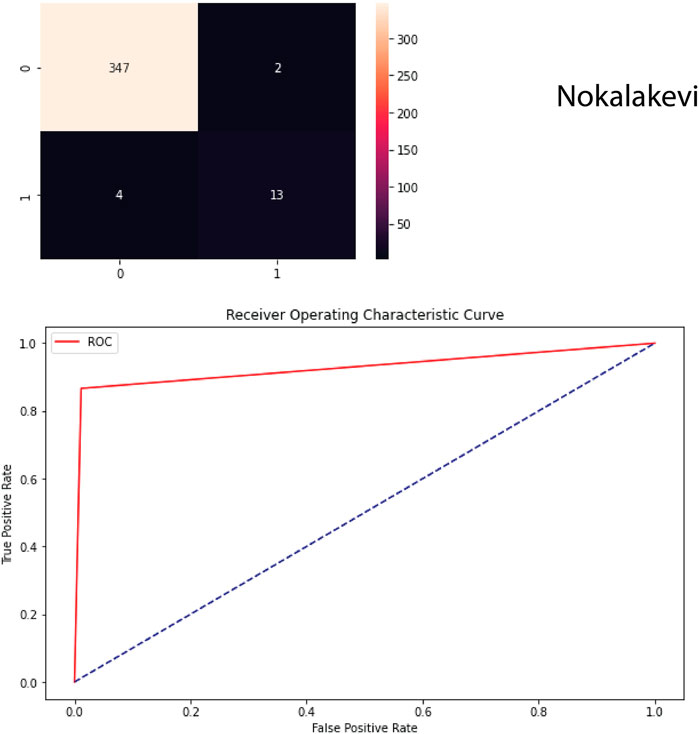
FIGURE 6. Confusion matrix (upper graph) and ROC curve (lower graph) obtained at forecasting the next day EQs of M=>3.5 in the area with the radius 200 km around the Nokalaqevi borehole using the previous day data. According to the confusion matrix, ML success cases amount to 12 from total 14 events with two false forecasts.

We carried out similar calculations for all five regions and compiled the confusion matrixes and averaged ROC AUC, where the observed imbalanced dataset was transformed into a balanced one. According to the confusion matrix, ML success cases amount to 12 from total 14 events with 2 false forecasts, that is, the hit rate is 0.86, which is quite encouraging.

Presented results show that machine learning allows forecasting the next day EQs of magnitude 3.5 and larger in the 200 km area around the well in the Noqalaqevi region with a high probability.

Apart from DT, we also tried the SVM program for forecasting EQ using the same training/testing datasets—the results were close to these of the DT approach. Exactly, by the SVM, we obtained slightly less (by 2%) successfully forecasted seismic events. Therefore, we do not present these results in detail here.

4.2.3 Forecast of the Next Day Earthquakes of the Fifth Independent Region Using Previous Day Data of Other Four Regions and Robust Metrics (MCC, ROC)

Using the same approach, we can consider any four of five regions as a training base and the fifth one—as a target (test) region. In this way, we were able to test the validity of the chosen model in more or less independent way to other four regions. Using the results of the earlier analysis, we present as the confusion matrix (Table 2) forecasting EQs of $M\ge 3.5$ in the area with radius 200 km around the Axalkalaki, Adjamerti, Marneuli, and Kobuleti boreholes for 2020.

TABLE 2

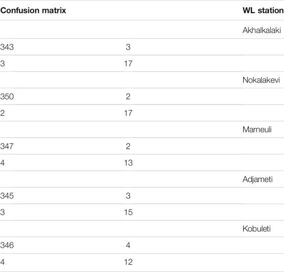
TABLE 2. Final confusion matrixes calculated on the original EQ data of four target stations using the remaining four stations as the training set.

It is evident that in addition to good enough forecasting the model demonstrates in the training region—Nakalakevi (Figures 6A,B), it reveals applicability to the other four testing areas (Table 2); otherwise, taking into account the existing strong imbalance, it would be impossible to achieve forecasting of most of the occurred EQ events.

5 Choosing Appropriate Metrics for the Imbalanced Datasets

In solving the ML binary classification problem for the rare events, it is important to use the correct metrics, which takes into account the imbalance of the datasets (Mena and Gonzalez 2006; Johnson and Khoshgoftaar 2019; Malik and Ozturk, 2020). Previously, we show that the accuracy is not a good classifier, if there are high TN values. Chicco and Jurman (2020) and Chicco et al. (2021) show that in addition to accuracy, F1 also provides misleading information, though some authors claim that it is applicable to imbalanced data.

The appropriate metrics for the imbalanced data case is the Matthews’ correlation coefficient (MCC), a special case of the phi (φ) coefficient (Matthews, 1975; Chicco and Jurman, 2020; Chicco et al., 2021):

$MCC=\frac{TP\times TN-FP\times FN}{\surd \left(TP+FP\right)\left(TP+FN\right)\left(TN+FP\right)\left(TN+FN\right)}.(2)$

The MCC varies in the range (−1, 1); the model is optimal if the MCC = 1. The MCC classifier is preferable to use, when the statistics of both negative and positive classes are important for the prediction problem. The MCC is a balanced measure, which can be used even if the negative and positive classes are of very different sizes. MCC close to +1 provides high values of all main parameters of the confusion matrix.

Let us consider the results of application of the MCC classifier (Table 3). It is evident that the results of the MCC test for the original data indicate that the applied methodology allows forecasting events of $M\ge 3.5$ quite satisfactorily—the values of the MCC are close to one. According to Chicco and Jurman (2020), the MCC criterion gives correct predictions on a majority of both positive and negative cases independent on their ratios in the dataset. On the other hand, in the following article, Chicco et al. (2021) conclude that “if the positive data instances are more important than negative elements in classification (both for ground truth classification and for predictions), the F1 score can be more relevant than the MCC.” As we believe that the correct prediction of positive cases—“events”—are more important than correct prediction of negative cases—“quiet days,” below in Table 3, we present the corresponding scores for F1 also and several other characteristics: accuracy, precision, and recall, using the confusion matrix data (Table 3).

TABLE 3

TABLE 3. Classification performance measures in EQ forecast: MCC, accuracy, precision, recall, and F1

From the data presented in Table 3, it follows that the values of the MCC, precision, recall, and F1 score are close to each other, when the accuracy assessment is overoptimistic due to the negligence of significant imbalance in the data (large values of true negatives TN—see Eq. 1 and comments below).

6 Testing MCC Results: Randomization of EQ Catalog

For testing the MCC approach validity, we randomized the input training data for the Nakalakevi station. In order to assess the accuracy of our approach, we used the following method: the 32 columns with training data were held constant and only in the testing data on EQs dates of events were randomized. Namely, in the majority (aseismic) datasets, we implanted randomly the additional seismic events according to the following rule: in the middle of the quiet days cluster, we placed one event of$M\ge 3.5$. According to the theory, the MCC for randomized datasets should decrease significantly, taking values close to zero or (−1). In the following text, we show the results of MCC testing on the randomized Nokalakevi station data. The MCC for original data is 0.851. After randomization the MCC test shows (Figure 7) that for the Nokalalkevi station, the MCC value is very small: MCC = 0.174, which means that the applied forecasting method is quite promising.

FIGURE 7

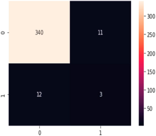
FIGURE 7. Confusion matrix for the randomized training EQ catalog at the Nokalakevi station—the timings of EQs in the corresponding output column are randomized (the occurrence times were displaced according to the rule—see before). Compare with the original Figure 6A.

7 Future Research

It seems promising in the future research to include more predictors, expand the training/testing periods, and aim to the forecast of stronger events, namely, one could try the following schemes of forecast: including dataset of weak seismic events of M less than 3.5 in the predictors’ list (class); expanding the predicting datasets of weak seismicity, WL, magnetic, etc. for several years; expanding the training input interval to several days; using longer seismic catalogs; and forecasting stronger events (magnitudes $M\ge 3.5$). It is also interesting to operate the model in the real-time regime, namely, to give a (zero or one)-type forecast of the event of $\text{M}\ge 3.5$ on the distance of 200 km from a well for the next day using the previous day data.

8 Conclusion

The problem of the next-day forecast for events of $M\ge 3.5$ in Georgia and elsewhere should take into consideration the imbalance between the days with earthquakes and quiet days in the output data. For example, the ratio of seismic to aseismic days for in Georgia reaches the values of the order of 1:20 and more, which mean that the dataset is significantly imbalanced. In this case, some accepted ML classification measures, such as accuracy, lead to wrong predictions due to a large weight of true negative cases. As a result, the minority class, here—the seismically active periods—is ignored at all. We applied specific measures to avoid the imbalance effect and exclude the overfitting possibility. After regularization (balancing) of the training data, we build the confusion matrix and performed receiver operating classification in order to forecast the next-day probability of $M\ge 3.5$ earthquake occurrence. We found that Matthews’ correlation coefficient (MCC) gives good results even if the initially negative and positive classes are of very different sizes, namely, the next day $M\ge 3.5$ seismic event probability is of the order of 0.8. After randomization of EQ dates in the training dataset, the Matthews coefficient efficiency decreases to 0.17.

Data Availability Statement

The raw data supporting the conclusions of this article will be made available by the authors, without undue reservation.

Author Contributions

TC contributed to the sections “Introduction,” “Methodology,” “Networks, Devices, and Data,” “Results,” “Choosing Appropriate Metrics for the Imbalanced Datasets,” and “Conclusions.” TK contributed to the sections “Machine Learning (ML) Methodology,” “Results,” “ML Algorithms,” and “Testing MCC Results: Randomization of EQ Catalog.” GM, GK, and TJ contributed to the sections “Networks, Devices, and Data” and “Machine Learning (ML) Methodology.” All authors contributed to the article and approved the submitted version.

Conflict of Interest

The authors declare that the research was conducted in the absence of any commercial or financial relationships that could be construed as a potential conflict of interest.

Publisher’s Note

All claims expressed in this article are solely those of the authors and do not necessarily represent those of their affiliated organizations, or those of the publisher, the editors, and the reviewers. Any product that may be evaluated in this article, or claim that may be made by its manufacturer, is not guaranteed or endorsed by the publisher.

References

Balasis, G., Daglis, I. A., Anastasiadis, A., Papadimitriou, C., Mandea, M., and Eftaxias, K. (2011). Universality in Solar Flare, Magnetic Storm and Earthquake Dynamics Using Tsallis Statistical Mechanics. Physica A 390, 341–346. doi:10.1016/j.physa.2010.09.029

CrossRef Full Text | Google Scholar

Bottou, L., and Bousquet, O. (2012). “The Tradeoffs of Large Scale Learning,” in Optimization for Machine Learning. Editors S. Sra, S. Nowozin, and S. Wright (Cambridge: MIT Press), 351–368.

Google Scholar

Brownlee, J. (2021). Imbalanced Classification with Python: Better Metrics, Balance Skewed Classes, Cost-Sensitive Learning. Kindle Edition. Amazon. Available at: https://amzn.to/3s4Ihfb

Google Scholar

Brunton, S., and Kutz, J. (2020). Data-Driven Science and Engineering. Cambridge, United Kingdom: Cambridge University Press, 492.

Google Scholar

Buchachenko, A. (2021). Magnetic Control of the Earthquakes. Open J. Earthquake Res. 10, 138–152. doi:10.4236/ojer.2021.104009

CrossRef Full Text | Google Scholar

Chawla, N., Herrera, F., Garcia, S., and Fernandez, A. (2018). SMOTE for Learning from Imbalanced Data: Progress and Challenges, Marking the 15-year Anniversary. J. Artif. Intelligence Res. 61, 863–905. doi:10.1613/jair.1.11192

CrossRef Full Text | Google Scholar

Chelidze, T., Melikadze, G., Kiria, T., Jimsheladze, T., and Kobzev, G. (2020). Statistical and Non-linear Dynamics Methods of Earthquake Forecast: Application in the Caucasus. Front. Earth Sci. 8, 194. doi:10.3389/feart.2020.00194

CrossRef Full Text | Google Scholar

Chelidze, T., and Matcharashvili, T. (2015). “Dynamical Patterns in Seismology,” in Recurrence Quantification Analysis. Editors C. Webber, and N. Marwan (Springer), 291–335. doi:10.1007/978-3-319-07155-8_10

CrossRef Full Text | Google Scholar

Chelidze, T., Melikadze, G., Kobzev, G., La, S., Nato, J., and Ekaterine, M. (2019). Hydrodynamic and Seismic Response to Teleseismic Waves of strong Remote Earthquakes in Caucasus. Acta Geophysica 67, 1–16. doi:10.1007/s11600-018-00241-7

CrossRef Full Text | Google Scholar

Chelidze, T., Sobolev, G., Kolesnikov, Y., and Zavjalov, A. (1995). Seismic hazard and Earthquake Prediction Research in Georgia. J. Georg. Geophys. Soc. 1A, 7–39.

Google Scholar

Chicco, D., and Jurman, G. (2020). The Advantages of the Matthews Correlation Coefficient (MCC) over F1 Score and Accuracy in Binary Classification Evaluation. BMC Genomics 21, 6. doi:10.1186/s12864-019-6413-7

PubMed Abstract | CrossRef Full Text | Google Scholar

Chicco, D., Tutsch, N., and Jurman, G. (2021). The Matthews Correlation Coefficient (MCC) Is More Reliable Than Balanced Accuracy, Bookmaker Informedness, and Markedness in Two-Class Confusion Matrix Evaluation. BioData Mining 14, 13. doi:10.1186/s13040-021-00244-z

PubMed Abstract | CrossRef Full Text | Google Scholar

Dobrovolsky, I., Zubkov, S., and Miachkin, V. (1979). Estimation of the Size of Earthquake Preparation Zones. Pure Appl. Geophys. 117, 1025–1044. doi:10.1007/bf00876083

CrossRef Full Text | Google Scholar

Dvorkin, J., Nolen-Hoeksema, R., and Nur, A. (1994). The Squirt-flow Mechanism: Macroscopic Description. Geophysics 59, 428–438. doi:10.1190/1.1443605

CrossRef Full Text | Google Scholar

Fernández, A., García, S., and Galar, M. (2018). Learning from Imbalanced Data Sets. Heidelberg, Germany: Springer. doi:10.1007/978-3-319-98074-4

CrossRef Full Text | Google Scholar

He, H., and Garcia, E. A. (2009). Learning from Imbalanced Data. IEEE Trans. Knowledge Data Eng. 21 (9), 1263–1284. doi:10.1109/tkde.2008.239

CrossRef Full Text | Google Scholar

Johnson, J., and Khoshgoftaar, T. (2019). Survey on Deep Learning with Class Imbalance. J. Big Data 6, 27. doi:10.1186/s40537-019-0192-5

CrossRef Full Text | Google Scholar

Johnson, P. A., Rouet-Leduc, B., Pyrak-Nolte, L., Marone, C. J., Hulbert, C., Howard, A., et al. (2021). Laboratory Earthquake Forecasting: A Machine Learning Competition. PNAS 118 (5), e2011362118. doi:10.1073/pnas.2011362118

PubMed Abstract | CrossRef Full Text | Google Scholar

Karpathy, A. (2017). A Peek at Trends in Machine Learning. Available online at: https://medium.com/@karpathy/a-peek-at-trends-in-machine-learningab8a1085a106 (accessed June 12, 2020).

Google Scholar

Kingma, D., and Ba, J. (2014). Adam: A Method for Stochastic Optimization. Available online at: http://arxiv.org/abs/1412.6980http://arxiv.org/abs/1412.6980 (accessed May 12, 2020).

Google Scholar

Malik, N., and Ozturk, U. (2020). Rare Events in Complex Systems: Understanding and Prediction. Chaos 30, 090401. doi:10.1063/5.0024145

PubMed Abstract | CrossRef Full Text | Google Scholar

Matthews, B. W. (1975). Comparison of the Predicted and Observed Secondary Structure of T4 Phage Lysozyme. Biochim. Biophys. Acta (BBA) Protein Struct. 405 (2), 442–451. doi:10.1016/0005-2795(75)90109-9

CrossRef Full Text | Google Scholar

Mena, L., and Gonzalez, J. (2006). “Machine Learning for Imbalanced Datasets: Application in Medical Diagnostic,” in Proceedings of the Nineteenth International Florida Artificial Intelligence Research Society Conference, Melbourne Beach, Florida, USA, May 11-13, 2006. Available at: https://www.researchgate.net/publication/221438576.

Google Scholar

Mitchell, T. (1997). Machine Learning. New York: McGraw-Hill. 0-07-042807-7.OCLC 36417892

Google Scholar

Pedregosa, F., Varoquaux, G., Gramfort, A., Michel, V., Thirion, B., Grisel, O., et al. (2011). Scikit-learn: Machine Learning in Python. J. Machine Learn. Res. 12, 2825–2830.

Google Scholar

Prejean, S., and Hill, D. (2009). “Dynamic Triggering of Earthquakes,” in Encyclopedia of Complexity and Systems Science. Editor A. Meyers (Berlin: Springer), 2600–2621. doi:10.1007/978-0-387-30440-3_157

CrossRef Full Text | Google Scholar

Ren, C. X., Hulbert, C., Johnson, P. A., and Roulet-Leduc, B. (2020). “Machine Learning and Fault Rupture: A Review,” in Advances in Geophysics (Amsterdam, Netherlands: Elsevier), 61. Available at: https://www.researchgate.net/publication/342216700.

CrossRef Full Text | Google Scholar

Rouet-Leduc, B., Hulbert, C., Bolton, D. C., Ren, C. X., Riviere, J., Marone, C., et al. (2018). Estimating Fault Friction From Seismic Signals in the Laboratory. Geophys. Res. Lett. 45 (3), 1321–1329. doi:10.1002/2017GL076708

CrossRef Full Text | Google Scholar

Rouet-Leduc, B., Hulbert, C., Lubbers, N., Barros, K. M., Humphreys, C., and Johnson, P. A. (2017). Machine Learning Predicts Laboratory Earthquakes. Geophys. Res. Lett. 44. doi:10.1002/2017GL074677

CrossRef Full Text | Google Scholar

T. Chelidze, F. Valliantos, and L. Telesca (Editors) (2018). Complexity of Seismic Time Series (Amsterdam, Netherlands: Elsevier). doi:10.1016/B987-0-12-813138-1-00009-2

CrossRef Full Text | Google Scholar

Vapnik, V., and Chervonenkis, A. (1974). Pattern Recognition Theory, Statistical Learning Problems. Moskva: Nauka Publisher.

Google Scholar

V. Vapnik (Editor) (1984). Algorithms and Programs for Recovering Dependences (Moscow: Nauka Publisher).

Google Scholar

Wang, C.-Y., and Manga, M. (2010). Earthquakes and Water. Heidelberg, Germany: Springer, 225.

Google Scholar

Witten, I., Frank, E., Hall, M., and Pal, C. (2017). Data Mining: Practical Machine Learning Tools and Techniques (Morgan Kaufmann Series in Data Management Systems). 4th Edition. Amsterdam, Netherlands: Elsevier.

Google Scholar

Zavjalov, A. (2006). Middle-term Earthquake Prediction. Moscow: Nauka Publisher.

Google Scholar

Zotov, O., Guglielmi, A., and Sobisevich, A. (2013). On Magnetic Precursors of Earthquakes. Izvestiya, Phys. Solid Earth 49 (6), 882–889. doi:10.1134/s1069351313050145

CrossRef Full Text | Google Scholar