Diffraction Extraction and Least-Squares Reverse Time Migration Imaging for the Fault-Karst Structure With Adaptive Sampling Strategy

The ultra-deep fault-karst structure discovered in the Tarim Basin in Western China is a fractured-vuggy carbonate reservoir with great potential for development. The diffraction generated by fractures, small-scale caves and vugs is often used for reservoir identification and seismic interpretation. Since the diffraction is much weaker than the reflection, it is difficult to separate the diffraction from the full wavefield. We use a plane-wave destruction (PWD) filter to extract the diffraction from the full data. In order to obtain a high-accuracy and amplitude-preserving imaging profile, we use the least-squares reverse time migration (LSRTM) method to image the separated diffraction. The large amount of calculation is the most challenging problem of the LSRTM algorithm. In view of this, we develop an adaptive sampling strategy to improve computing efficiency and reduce memory requirement. We use a fault model, a vugs-fractures model, and a fault-karst model to demonstrate the effectiveness and practicability of the proposed method. The numerical examples show that the proposed method can enhance the imaging resolution of the fault-karst structure and save computing cost without losing accuracy. In addition, a test on field data processing demonstrates the advantages of our algorithm.

Introduction

The marine carbonate reservoirs have produced abundant oil and gas resources globally (Loucks and Anderson, 1985; Soudet et al., 1994; Tian et al., 2016). Their formation is related to faulting and dissolution. Different from conventional fractured carbonate reservoirs, the ultra-deep fault-karst reservoirs discovered in the Shunbei area of the Tarim Basin are controlled by large-scale faults, karstification and deep hydrothermal reforming (Li et al., 2019). The reservoirs are dominated by various irregular vugs and fractures occurring along the large-scale strike-slip faults or the associated secondary faults. According to structural features and controlling factors, Lu et al. (2015) first proposed the theoretical concept of fault-karst traps, and divided the fault-karst reservoirs into three categories. Ma et al. (2019) summarized the reflection characteristics of the fault-karst structure using forward modeling, which provides guidance for its identification. However, due to deep burial depth and complex inner structure, the diffraction generated by vugs or fractures is much weaker than the reflection, making it difficult to obtain high-resolution seismic imaging profile (Khaidukov et al., 2004; Kong et al., 2017). Furthermore, the large amount of computational cost caused by large-scale and high-precision imaging process is inevitable. In view of the above, a more accurate and efficient imaging method is needed to support the exploration and development of the ultra-deep fault-karst reservoirs.

Separating the diffraction from full wavefield is very important for the high-resolution imaging of the fault-karst structure. The differences between reflected waves and diffracted waves in kinematics are substantial in the common-shot gathers, which allows us to extract the diffraction from the shot records (Landa et al., 1987). Dip filtering (Bansal and Imhof, 2005), focusing and defocusing (Khaidukov et al., 2004) hybrid Radon transform (Klokov et al., 2010), and PWD filtering (Fomel, 2002; Taner et al., 2006) have been developed for separating diffraction. These methods utilized the fact that the travel time curve of the diffracted wave is quasi-parabolic in the common-shot gathers while the reflected wave is quasi-linear. The PWD filtering method can effectively eliminate artifacts and retain more diffraction energy. Therefore, it has been successfully applied to several 3D field datasets (Burnett et al., 2015; Tyiasning et al., 2016). Another advantage of the PWD filtering method is that the separated diffraction can be directly used for pre-stack migration, avoiding complex data processing.

Reverse time migration (RTM), which is based on two-way wave equation, can effectively migrate reflection data and describe subsurface geological structures (Baysal et al., 1983; Sun and McMechan, 1986). LSRTM can be regarded as the optimization algorithm of RTM. It employs the least-squares inversion theory that continuously fits the error between the linear demigration data and the observed data (Tarantola, 1984; Nemeth et al., 1999; Dai et al., 2012). Compared to RTM, LSRTM can improve migration resolution, balance imaging amplitude, and reduce image artifacts (Dutta and Schuster, 2014; Yang et al., 2019). Nevertheless, this algorithm requires a huge amount of storage space and computational effort. Some researchers have tried to use different acceleration algorithms to improve LSRTM, such as multi-source and plane-wave encoding methods (Dai et al., 2012; Huang and Schuster, 2012; Dai and Schuster 2013). However, the crosstalk noise caused by different sources is hard to be eliminated.

Variable-grid methods, which are implemented by decreasing the grid points of a model, can reduce memory costs and improve computational efficiency (Moczo, 1989; Jastram and Behle, 1992; Fan et al., 2015; Huang et al., 2015). Several variable-grid methods have shown their potential in imaging. Li et al. (2014) developed a dual-variable grid algorithm and applied it to RTM. Li et al. (2017) introduced the idea of pseudo-time domain (Alkhalifah, 2003; Ma and Alkhalifah, 2013) into LSRTM, which improves imaging efficiency by reducing vertical grid points (Wang et al., 2020). Proposed an adaptive grid discretization strategy and applied it to 3D LSRTM. Most variable-grid methods always resample a local region. Due to the inherent difficulty of automatically discretizing spatial grid, local variable-grid methods have not been widely used in seismic data processing.

Diffraction extraction, high-resolution imaging, and cost control are key to accurate exploration of the ultra-deep fault-karst reservoirs. In this paper, we first apply the PWD filter method (Taner et al., 2006) to extract the diffraction from the full wavefield. Then, the diffraction-based LSRTM (D-LSRTM) algorithm are used to image the diffraction. In order to improve the computing efficiency, we develop an efficient variable-grid D-LSRTM method based on a globally adaptive sampling strategy (AS-D-LSRTM). Finally, four numerical tests are used to prove the effectiveness and robustness of the proposed method.

The complete workflow of the AS-D-LSRTM method is divided into the following steps: 1) separating the diffraction from the full wavefield by PWD filter method; 2) performing irregular grid discretization applying adaptive sampling; 3) imaging the diffraction using LSRTM.

The Principle of Diffraction Separation

In the common-shot gathers, the reflection and the diffraction generated by a point source share similar kinematic characteristics, which are difficult to be distinguished (Landa et al., 1987). While when the incident wave is a plane wave, the travel time curve of the reflected wave can be written as:

$t_R=\frac{\cos \theta \sin \left(\theta -2\varphi \right)}{v\cos \left(\theta -\varphi \right)}\cdot x+\frac{2h}{v}\left[\cos \theta \cos \left(\theta -\varphi \right)-\frac{cos\varphi \cos \left(\theta -\varphi \right)-\cos \theta }{\cos \left(\theta -\varphi \right)}\right](1)$

where $t_R$ denotes the travel time and $v$ denotes the medium velocity. The specific meaning of $\theta$ and $\varphi$ is shown in Figure 1.

FIGURE 1

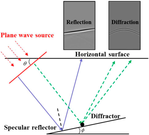
FIGURE 1. Comparison of the reflection and the diffraction. As illuminated by the plane wave source, the seismic response of the reflection is linear while the response of the diffraction is hyperbolic.

The travel time curve of the diffracted wave can be expressed as:

$\frac{{\left(t_D-h/v\right)}^2}{{h^2{\cos }^2\theta /v}^2}-\frac{{\left(x-h\sin \theta \right)}^2}{h^2{\cos }^2\theta }=1(2)$

According to Eqs. 1, 2 and Figure 1, the seismic response of the reflection is linear while the response of the diffraction is hyperbolic. Therefore, we can separate the reflection and the diffraction based on the difference of kinematic properties in plane-wave gathers. Firstly, we convert the common-shot gathers into common ray-parameter gathers using tau-p transform (Kappus et al., 1990; Zhang et al., 2005). The tau-p transform equation can be expressed as:

$P\left(\tau ,p\right)=\int d\left(t,x\right)dx=\int d\left(\tau +px,x\right)dx(3)$

where $d\left(t,x\right)$ denotes the seismic shot records in the time-offset $t-x$ domain, and $P\left(\tau ,p\right)$ is the so-called plane-wave gathers with ray parameter $p$ and time axis $\tau$. Then we use the PWD wave filter proposed by Fomel (2002) to estimate the local dip angle of the diffracted wave and separate it in the tau-p domain. After that, we use the inverse tau-p transform to get the diffraction wavefield in the time-offset domain. The inverse tau-p transform equation is expressed as:

$d_D\left(t,x\right)=\int P\left(\tau ,p\right)dp=\int P\left(\tau =t-px,p\right)dp(4)$

where $d_D\left(t,x\right)$ denotes the shot records of the diffracted wave.

Adaptive Sampling Strategy

In Tarim Basin, where the fractured-vuggy carbonate reservoirs are extensively developed, the surface is often covered by desert and gravel layers with low velocity. In forward modeling and migration, a fine spatial grid must be used to avoid numerical dispersion. However, for the deep region with high velocity, using fine grid is a waste of computing resources. We use an adaptive sampling strategy to solve the above problem.

As shown in Figure 2, the horizontal axis denotes depth and the vertical axis represents vertical grid interval. The black dots on the x-axis denote initial vertical grid points. The black solid line denotes initial vertical grid interval, which is fixed. According to the medium velocity and the dominant frequency of the source, we use Eq. 5 to recalculate the optimal vertical grid interval (The red solid line in Figure 2):

$dz\left(z\right)=\frac{v_{\min }\left(z\right)}{10f_m}(5)$

where $v_{\min }\left(z\right)$ denotes the minimum velocity along the depth axis z, $f_m$ is the dominant frequency of the source wavelet, and $dz\left(z\right)$ denotes the optimal vertical grid spacing.

FIGURE 2

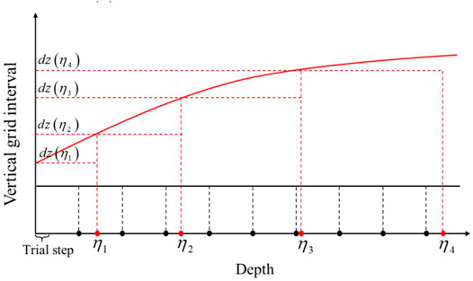
FIGURE 2. Diagrammatic sketch of the adaptive sampling method.

We use a rectangular sampling method (Wang et al., 2020) to resample the initial migration model. Firstly, we set a small trial step from $z=0$ and increase it continuously to get the first grid point ${\eta }_1$, where ${\eta }_1=dz\left({\eta }_1\right)$. Then we repeat the previous step to get the second grid point ${\eta }_2$, where ${\eta }_2-{\eta }_1=dz\left({\eta }_2\right)-dz\left({\eta }_1\right)$. Finally, we repeat the above process to the max depth and obtain a new model. The vertical grid interval of the new model is irregular and it varies with velocity. Note that there is a mapping relationship between the initial model and the new model, we use two different coordinate systems to express it:

$x=x\left(\xi ,\eta \right)(6)$

$z=z\left(\xi ,\eta \right)(7)$

where $x$ and $z$ are the coordinate variables in coordinate system $A\left(x,z\right)$, $\xi$ and $\eta$ are the coordinate variables in coordinate system $B\left(\xi ,\eta \right)$. The initial model is located in $A\left(x,z\right)$ and the new model is located in $B\left(\xi ,\eta \right)$. The derivation process of the mapping relationship is shown in Supplementary Appendix SA.

The acoustic wave equation in 2D heterogeneous isotropic medium in coordinate system $A\left(x,z\right)$ can be written as:

$\frac{1}{v^2}\frac{{\partial }^{2}u}{\partial t^2}=\rho \left(\frac{{\partial }^{2}u}{\partial x^2}+\frac{{\partial }^{2}u}{\partial z^2}\right)+f_s\left(t\right)(8)$

where u denotes acoustic pressure field, t denotes time, ρ denotes medium density, v denotes acoustic velocity, and $f_s\left(t\right)$ denotes source function.

Substitute Eq. A-9 and A-10 into Eq. 8, we get the expression of Eq. 8 in coordinate system $B\left(\xi ,\eta \right)$:

$\frac{1}{v^2}\frac{{\partial }^{2}u}{\partial t^2}=\rho \left(\frac{{\partial }^{2}u}{\partial {\xi }^2}+\frac{{\partial }^{2}u}{\partial {\eta }^2}\frac{1}{z_{\eta }^2}-\frac{\partial u}{\partial \eta }\frac{z_{\eta \eta }}{z_{\eta }^3}\right)+f_s\left(t\right)(9)$

where $z_{\eta }=\partial z/\partial \eta$ and $z_{\eta \eta }={\partial }^{2}z/\partial {\eta }^2$ they can be solved by finite-difference method.

Compared to Eq. 8, one term is added to Eq. 9, which increases the computational cost for one grid point. In fact, the omission of the extra term has little effect on the final imaging results. Therefore, Eq. 9 is further simplified as:

$\frac{1}{v^2}\frac{{\partial }^{2}u}{\partial t^2}=\rho \left(\frac{{\partial }^{2}u}{\partial {\xi }^2}+\frac{{\partial }^{2}u}{\partial {\eta }^2}\frac{1}{z_{\eta }^2}\right)+f_s\left(t\right)(10)$

Review of the Principle of LSRTM

LSRTM is considered to be a true amplitude imaging method, which can improve imaging resolution, reduce artifacts, and meet the demand for lithological interpretation.

As shown in Eq. 11, the seismic wavefield satisfies the superposition principle:

$u=u_0+u_s(11)$

where $u$ denotes total wavefield, $u_0$ denotes background wavefield, and $u_s$ denotes perturbation wavefield.

Similarly, the velocity model can be regarded as the superposition of a perturbation model and a smoothed background model,

$\frac{1}{v^2}=\frac{1}{v_0^2}+\frac{1}{\mathbf{\Delta }{v}^2}(12)$

$u_0$ obeys Eq. 10:

$\frac{1}{v^2}\frac{{\partial }^2{u}_0}{\partial t^2}=\rho \left(\frac{{\partial }^2{u}_0}{\partial {\xi }^2}+\frac{{\partial }^2{u}_0}{\partial {\eta }^2}\frac{1}{z_{\eta }^2}\right)+f_s\left(t\right)(13)$

Substitute Eq. 11 and Eq. 12 into Eq. 10, subtract Eq. 13, and apply Born approximation (Dai et al., 2012), we can obtain the control equation of

$\frac{1}{v_0^2}\frac{{\partial }^2{u}_s}{\partial t^2}=\rho \left(\frac{{\partial }^2{u}_s}{\partial {\xi }^2}+\frac{{\partial }^2{u}_s}{\partial {\eta }^2}\frac{1}{z_{\eta }^2}\right)-\frac{1}{\Delta v^2}\frac{{\partial }^2{u}_0}{\partial t^2}(14)$

Eq. 14 is the Born (linearized) forwarding modeling equation, and it can be rewritten as a matrix:

$d_s=Lm(15)$

where $L$ is the Born forwarding modeling operator, $m$ denotes model parameter, and $d_s$ denotes the Born-modeled data. We can get the migration image by using the the RTM operator:

$m_{mig}=L^T{d}_s(16)$

where $m_{mig}$ represents the imaging result. $L^T$ denotes the RTM operator, which is the conjugate transpose of $L$.

The goal of LSM theory is to minimize the objective function, which is defined as:

$J\left(m\right)=\frac{1}{2}{\Vert Lm-d_{obs}\Vert }_2^2(17)$

where $J\left(m\right)$ is the objective function, $d_{obs}$ denotes the observed data, and ${\Vert \cdot \Vert }_2^2$ is the L2-norm of a vector.

We use a conjugate-gradient algorithm (Dai et al., 2012) to solve the model parameter $m$, which is formulated as:

$\begin{array}{l}{g}^{k+1}=L^{\ast }\left[L{m}^k-d_{obs}\right]\\ {\beta }^{k+1}=\frac{{\left[g^{k+1}\right]}^{\ast }\left[C{g}^{k+1}\right]}{\left[g^k\right]\left[C{g}^k\right]}\\ z^{k+1}=C{g}^{k+1}+{\beta }^{k+1}{z}^k\\ a^{k+1}=\frac{{\left[z^{k+1}\right]}^{\ast }\left[g^{k+1}\right]}{{\left[L{z}^{k+1}\right]}^{\ast }\left[L{z}^{k+1}\right]}\\ m^{k+1}=m^k-a^{k+1}{z}^{k+1}\end{array}(18)$

where $k$ and $\text{*}$ denote iteration index and conjugate transpose of a matrix, $g^k$ and ${\beta }^k$ represent gradient and correction coefficient, $z^k$ and ${\alpha }^k$ denote conjugate gradient direction and step length, and $C$ denotes precondition operator.

In summary, the implementation of the AS-D-LSRTM method contains four main steps. The first step is to separate diffraction. The second step is to resample the initial model. The third step is to obtain the image after several iterations by LSRTM. Finally, we use linear interpolation to convert the final image from the coordinate system $B\left(\xi ,\eta \right)$ to coordinate system $A\left(x,z\right)$. Figure 3 shows the complete workflow of AS-D-LSRTM.

FIGURE 3

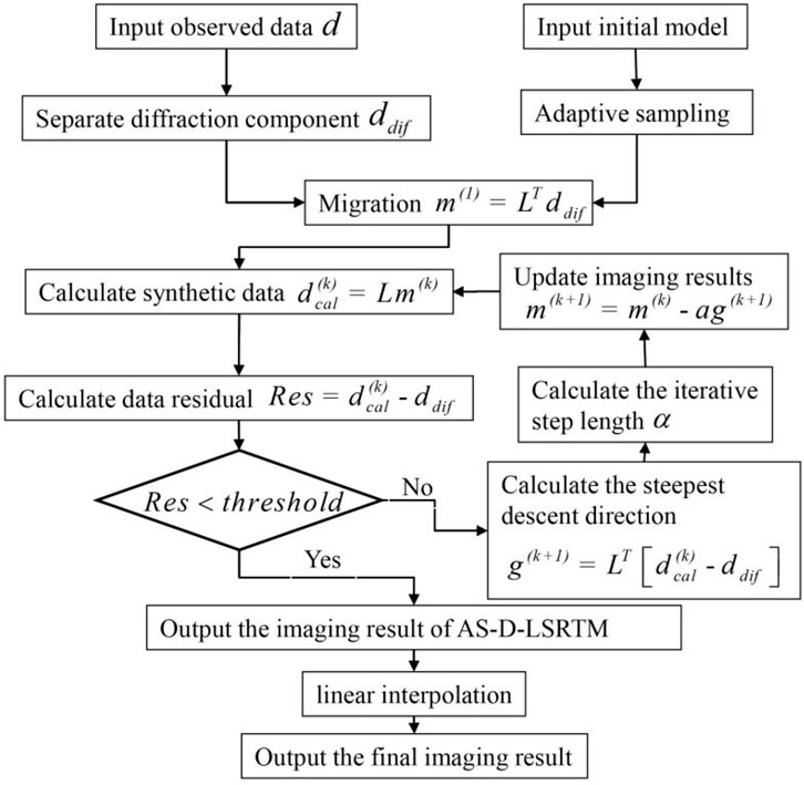
FIGURE 3. Workflow of AS-D-LSRTM.

Numerical Examples

In this section, three synthetic examples are used to test the effectiveness of the proposed AS-D-LSRTM in high-resolution imaging. Furthermore, numerical tests on land field data confirm its adaptability for complex structure.

Fault Model

The initial fault model is shown in Figure 4A, which has a low-velocity surface layer with velocity of 2000 m/s. It is discretized on a 801 × 301 grid a with grid spacing $dx=dz=$ 8 m. The time sampling interval is 0.5 ms and the recording time is 1.5 s. A total of 51 sources are distributed laterally from 2.4 to 4 km. The shot interval is 32 m. There are 601 receivers of each shot and the receiver interval is 8 m. We use a Ricker wavelet as the source, and its dominant frequency is 25 Hz. To improve the computational efficiency, we resample the initial model using the adaptive sampling method. Figure 4B shows the resampled model with 151 vertical grid points. From Figure 4B we can see that the deep layers with high velocity are compressed. Figure 5 shows the grid interval comparison of the two models. The black line in Figure 5 denotes initial vertical grid interval, the blue line denotes theoretical value calculated by Eq. 5, and the red line shows the vertical grid interval of the resampled model.

FIGURE 4

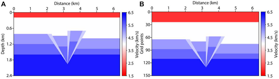
FIGURE 4. Fault model (A) and the resampled model (B).

FIGURE 5

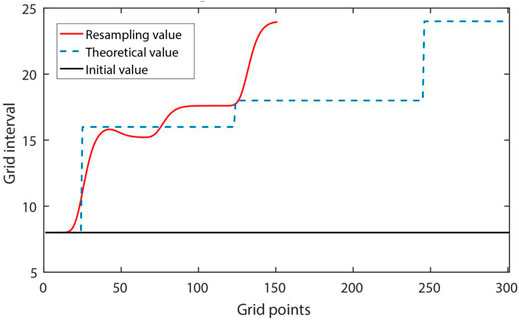
FIGURE 5. Comparison of vertical grid interval.

We use the tau-p transform to produce 501 plane-wave time sections with ray parameters ranging from −0.5 to 0.5 ms/m. Figure 6A displays a section with ray parameter $p=0$ ms/m. In Figure 6A, the reflection is linear (see the black arrows) and the diffraction is hyperbolic (see the red arrows). Figure 6B shows the estimated dip field of Figure 6A. Based on the dip angle field shown in Figure 6B, we use the PWD filter method to separate the diffraction. Figure 6C shows the separated diffraction with ray parameter $p=0$ ms/m. We can see from Figure 6C that the reflection is removed while the diffraction is preserved. Figure 7A shows the point source response of the full wavefield. In Figure 7A, the diffraction energy generated by the inclined faults (the red arrow) is much weaker than that of the layer interface (the black arrow). Figure 7B shows the response of the diffraction wavefield. In Figure 7B, the reflection is suppressed and the diffraction (the blue arrow) is preserved.

FIGURE 6

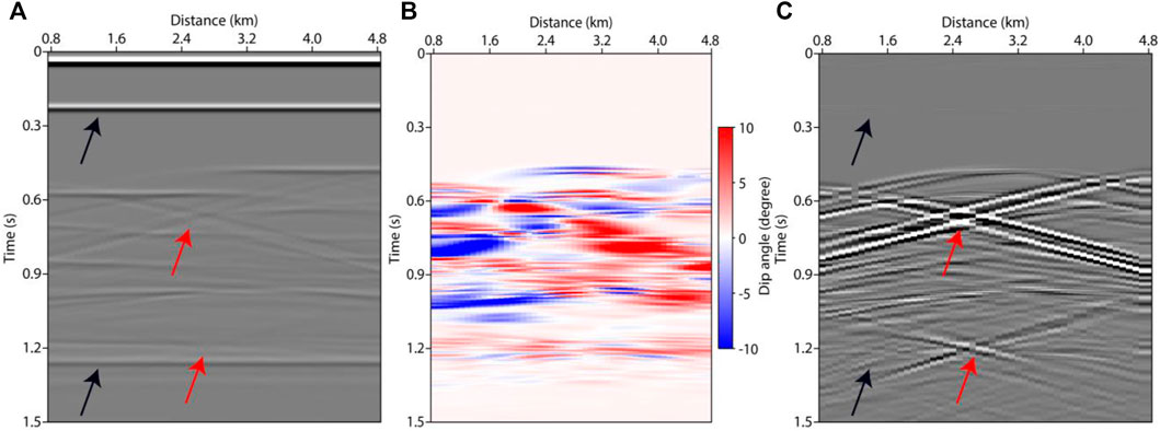
FIGURE 6. Time sections of the fault model with ray parameter $p=0$ ms/m. (A) plane-wave section for the full wavefield, (B) estimated dip angle field, and (C) plane-wave section for the separated diffraction.

FIGURE 7

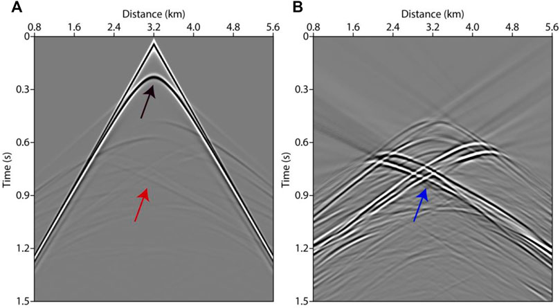
FIGURE 7. Response of the point source. (A) full wavefield, and (B) diffraction wavefield.

Figures 8A, 8B show the images of full wavefield LSRTM (F-LSRTM) and D-LSRTM after 30 iterations, respectively. In Figure 8B, we can see that the acquisition footprints (the red arrow) and the reflection generated by the surface layer (the blue arrow) are almost eliminated. Moreover, the resolution of the fault in Figure 8B is higher than that in Figure 8A (see the black arrows). Figure 8C shows the AS-D-LSRTM image after 30 iterations, and Figure 8D shows the final result after linear interpolation. In Figure 8B, the artifacts and the diffraction are enhanced simultaneously when the reflection is removed. Nevertheless, the diffraction-based LSRTM results are still focused. Figure 9 displays the normalized residual convergence curves of F-LSRTM, D-LSRTM, and AS-D-LSRTM. The curves show that the convergence rate of D-LSRTM and AS-D-LSRTM is faster than that of F-LSRTM. Moreover, the normalized residual of D-LSRTM and AS-D-LSRTM decreases quickly before the 5th iterations and gradually converges to a same value. Figure 10 shows the normalized computing time and memory footprint of these methods. Compared with D-LSRTM, AS-D-LSRTM can save 44% of computing cost and half of memory requirement without losing accuracy. From the above analysis, we conclude that AS-D-LSRTM is superior to F-LSRTM and D-LSRTM.

FIGURE 8

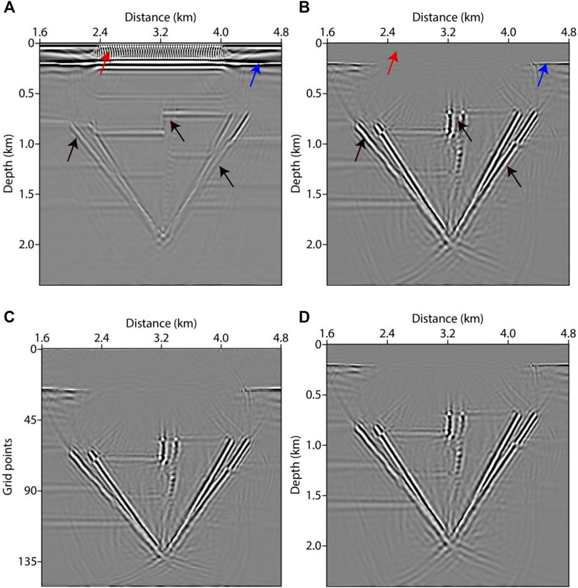
FIGURE 8. LSRTM images after 30 iterations using different methods. (A) F-LSRTM, (B) D-LSRTM, (C) AS-D-LSRTM, and (D) AS-D-LSRTM with linear interpolation.

FIGURE 9

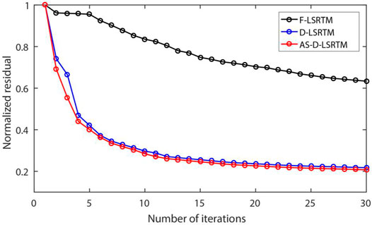
FIGURE 9. Normalized residual convergence curves of the three methods.

FIGURE 10

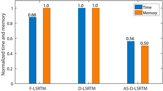
FIGURE 10. Computing time and memory requirement of the three methods.

Layered Model With Vugs and Fractures

We use a layered model to further verify the effectiveness of the proposed method. Figure 11A shows the initial model, which is discretized on a 801 × 401 grid with a grid interval of $dx=dz=$ 5 m. The model has two layers with velocity of 2.5 km/s and 4 km/s, respectively. There are three small-scale vugs and four fractures distributed at the layer interface with velocity of 3 km/s. The vugs are square with side lengths of 20, 40, and 60 m, respectively. The width of the fractures is 20 m and the lengths of them are 100, 200, 300, and 400 m, respectively. Figure 11B shows the resampled model ($f_m$ in Eq. 5 is 30), which has 221 vertical grid points in total. In total, 41 sources are distributed laterally from 1.5 to 2.5 km. Each shot has 601 receivers. The shot interval is 25 m and the receiver interval is 5 m. The time step is 0.3 ms and the recording time is 1.5 s.

FIGURE 11

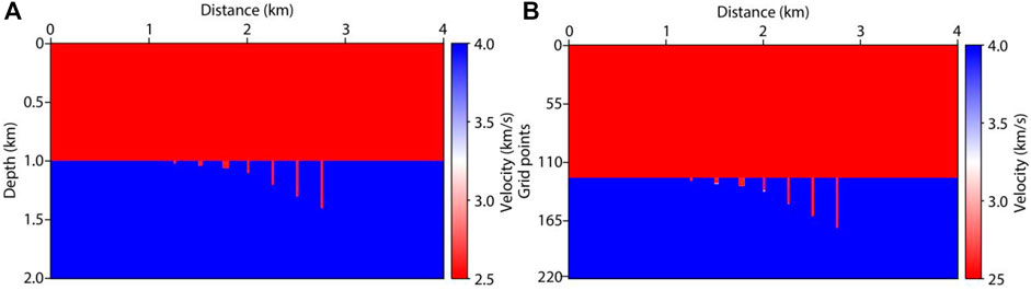
FIGURE 11. Fractures-vugs model (A) and the resampled model (B).

In this tests, we apply the adaptive sampling method to F-LSRTM (denoted by AS-F-LSRTM) and D-LSRTM. Figure 12 shows the images after 30 iterations using different LSRTM methods. In Figures 12A,C, the vugs and fractures are imaged successfully, and the bottom of the fractures is shown as a string of beads (Lu et al., 2015). In Figures 12B,D, the reflection are restrained and the energy of the diffraction is enhanced.

FIGURE 12

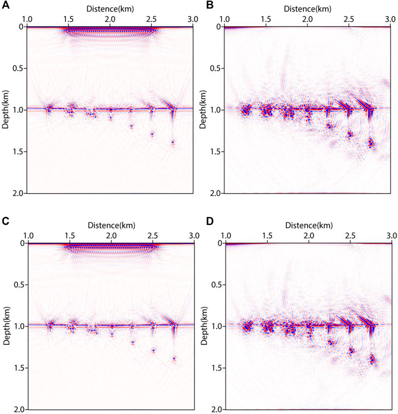
FIGURE 12. Migration images using different methods after 30 iterations. (A) F-LSRTM, (B) D-LSRTM, (C) AS-F-LSRTM with linear interpolation, and (D) AS-D-LSRTM with linear interpolation.

Figure 13 displays the normalized residual convergence curves of the four methods. The result shows that the convergence rate of D-LSRTM and AS-D-LSRTM is faster than that of F-LSRTM and F-AS-LSRTM. We can see that the convergence curves of D-LSRTM and AS-D-LSRTM are almost coincident after the 16th iteration. Figure 14 shows the normalized computing cost and storage requirement of the four methods. From Figures 12–14, we conclude that the AS-D-LSRTM algorithm is helpful to identify small-scale caves and fractures, and it can greatly save computing resources.

FIGURE 13

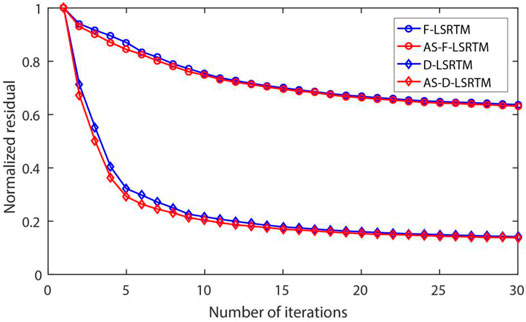
FIGURE 13. Normalized residual convergence curves of the four methods.

FIGURE 14

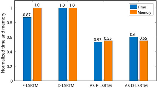
FIGURE 14. Computing time and memory requirement of the four methods.

Ultra-Deep Fault-Karst Carbonate Reservoir Model

The fault-karst carbonate reservoirs are usually stripped distribution along the strike-slip fault zone, especially in South Tahe area of Tarim Basin (Ding et al., 2020). According to stress state, the strike-slip fault can be divided into three structural styles, which are translation, extrusion and extension. The oil and gas resources are more abundant in the extension and extrusion section (Cheng et al., 2020). Figure 15 shows the distribution characteristics of the fault-karst reservoirs. In the extension section (left), large-scale caves are developed near the trunk fracture zone and small-scale vugs are distributed along the branch fracture. In the extrusion section (right), the caves and vugs are mainly distributed along the trunk fracture. According to the characteristics of the fault-karst carbonate reservoirs formed by strike-slip extension, we build an ultra-deep fault-karst model, as shown in Figure 16A. The model includes 1101 × 1101 grid points with grid spacing of 8 m. The maximum depth of the fault-karst structure is more than 8 km. Figure 16B shows the new model after adaptive sampling. The number of vertical grid points reduces from 1101 to 510.

FIGURE 15

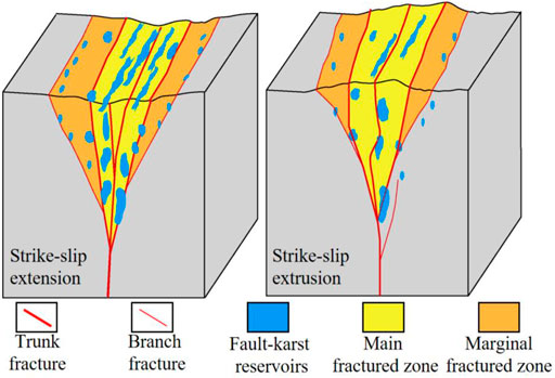
FIGURE 15. Distribution characteristics of the fault-karst carbonate reservoirs.

FIGURE 16

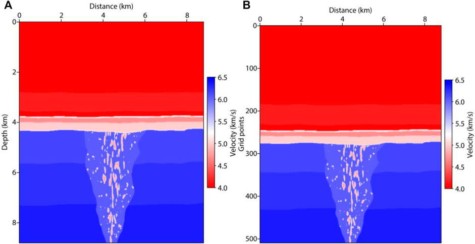
FIGURE 16. Ultra-deep fault-karst carbonate reservoir model (A) and the resampled model (B).

In numerical tests, a total of 61 sources are distributed laterally from 3.2 to 5.6 km. Each shot has 801 receivers. The shot interval is 40 m and the receiver interval is 8 m. The time step is 0.5 ms and the record time is 4 s. The source is a Ricker wavelet and its dominant frequency is 25 Hz. Figures 17A,B show AS-F-LSRTM and AS-D-LSRTM images after 20 iterations, respectively. In Figure 17A, some small-scale caves and vugs are shown as strong reflection spots (see the red arrows). However, the reflection energy generated by large-scale caves near the trunk fracture is much weaker (see the black arrows). In addition, the reflection-based LSRTM images cannot correctly describe the distribution and the structural characteristics of the fault-karst reservoirs. For example, the reflection energy of the top of the reservoirs is extremely weak (see the blue arrows in Figure 17A). This phenomenon can mislead the prospectors and lead them to miss productive reservoirs. In Figure 17B, the diffraction of the trunk fracture is much stronger than that in Figure 17A (see the black arrows). Moreover, the top of the reservoirs is easier to identify in Figure 17B (see the blue arrows). We conclude that AS-D-LSRTM can enhance the diffraction and improve the imaging resolution of the fault-karst carbonate reservoirs.

FIGURE 17

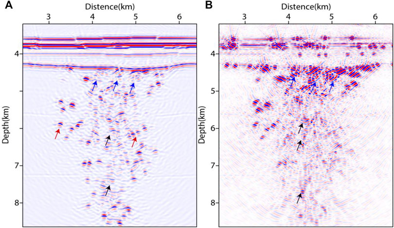
FIGURE 17. LSRTM images after 20 iterations. (A) AS-F-LSRTM and (B) AS-D-LSRTM.

Field Data Test

The LSRTM algorithms relies heavily on accurate migration velocity model and high-quality data. In this paper, the proposed AS-D-LSRTM method is also tested on a 2D field dataset to further verify its effectiveness. Figure 18A shows the initial migration velocity model, which includes 2001 × 401 grid points with a grid spacing of 10 m. Figure 18B shows the variable-grid model after adaptive sampling (n in Eq. 5 is 10), which is discretized on a 401 × 284 grid. We use the Ricker wavelet with dominant frequency of 20 Hz as the source. Total shots are 100 with irregular distribution and the record time is 4 s. Each shot has 204 receivers and the receiver interval is 50 m. The time sampling interval is 0.5 ms.

FIGURE 18

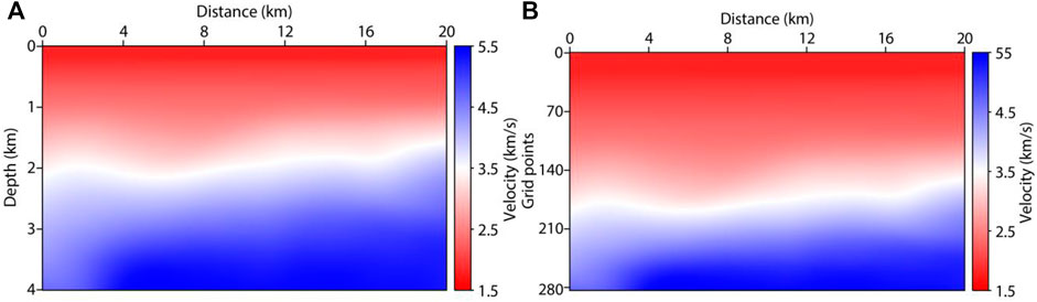
FIGURE 18. Initial migration velocity model (A) and (B) the resampled model.

Figure 19A shows a single shot record. We apply the PWD filter method to the full-wavefield data and obtain its diffraction component, as shown in Figure 19B. Figures 20A,B show the AS-F-LSRTM and AS-D-LSRTM images after 5 iterations, respectively. In Figure 20A, the diffraction generated by the fault (see the red arrow) is muck weaker than the reflection produced by the horizontal layers (see the black arrow). From the image result of AS-D-LSRTM (Figure 20B), we can see that the reflection energy (see the red arrow) is almost eliminated while the diffraction is enhanced (see the black arrow). In addition, about 74% of computing time and 71% of memory space are saved after using the adaptive sampling method. We conclude that our method is still effective for field data.

FIGURE 19

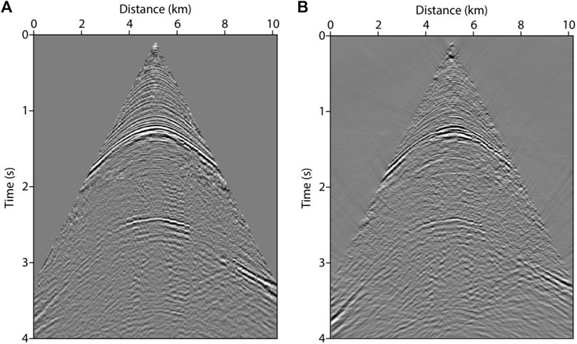
FIGURE 19. Field shot record. (A) full wavefield, and (B) diffraction wavefield.

FIGURE 20

FIGURE 20. Migration images after 5 iterations using AS-F-LSRTM (A) and AS-D-LSRTM (B).

Conclusion

We propose a high-accuracy and high-efficiency AS-D-LSRTM method, which contains three main parts. Firstly, we use the PWD filter to extract the diffraction from the full wavefield. Then we resample the initial migration model using the adaptive sampling strategy. Finally, we image the diffraction and obtain high-resolution migration results after multiple iterations. LSRTM is known to be limited by huge amount of computation when tens of iterations and hundreds of shots are required to be carried out. Numerical tests on synthetic data and field data demonstrate that the proposed AS-D-LSRTM method greatly improves computing efficiency and reduces memory requirement. In addition, our method can effectively image the diffraction produced by faults, fractures, caves and vugs. In summary, AS-D-LSRTM is a potential imaging approach for the interpretation and depiction of the fault-karst carbonate reservoirs in the Tarim Basin in Western China.

Data Availability Statement

The original contributions presented in the study are included in the article/Supplementary Material, further inquiries can be directed to the corresponding author.

Author Contributions

LC and JH contributed to the conception and design of the study. CS organized the database and performed the statistical analysis. JH modified the manuscript. All authors contributed to manuscript revision and read and approved the submitted version.

Funding

This research is supported by the National Key R&D Program of China (no. 2019YFC0605503), the National Outstanding Youth Science Foundation (no. 41922028), and the Major Scientific and Technological Projects of CNPC (no. ZD2019-183-003).

Conflict of Interest

The authors declare that the research was conducted in the absence of any commercial or financial relationships that could be construed as a potential conflict of interest.

Publisher’s Note

All claims expressed in this article are solely those of the authors and do not necessarily represent those of their affiliated organizations, or those of the publisher, the editors, and the reviewers. Any product that may be evaluated in this article, or claim that may be made by its manufacturer, is not guaranteed or endorsed by the publisher.

Acknowledgments

The authors are grateful to the editor and reviewers for reviewing this article.

Supplementary Material

The Supplementary Material for this article can be found online at: https://www.frontiersin.org/articles/10.3389/feart.2022.846034/full#supplementary-material

References

Alkhalifah, T. (2003). Tau Migration and Velocity Analysis: Theory and Synthetic Examples. Geophysics 68 (4), 1331–1339. doi:10.1190/1.1598126

CrossRef Full Text | Google Scholar

Bansal, R., and Imhof, M. G. (2005). Diffraction Enhancement in Prestack Seismic Data. Geophysics 70 (3), V73–V79. doi:10.1190/1.1926577

CrossRef Full Text | Google Scholar

Baysal, E., Kosloff, D. D., and Sherwood, J. W. C. (1983). Reverse Time Migration. Geophysics 48 (11), 1514–1524. doi:10.1190/1.1441434

CrossRef Full Text | Google Scholar

Burnett, W. A., Klokov, A., Fomel, S., Bansal, R., Liu, E., and Jenkinson, T. (2015). Seismic Diffraction Interpretation at Piceance Creek. Interpretation 3 (1), SF1–SF14. doi:10.1190/INT-2014-0091.1

CrossRef Full Text | Google Scholar

Cheng, H., W, Y., and Lu, X. B. (2020). Acta Petrolei Sinica 41 (3), 301–309. doi:10.7623/syxb202003005

CrossRef Full Text

Dai, W., Fowler, P., and Schuster, G. T. (2012). Multi-source Least-Squares Reverse Time Migration. Geophys. Prospecting 60 (4), 681–695. doi:10.1111/j.1365-2478.2012.01092.x

CrossRef Full Text | Google Scholar

Dai, W., and Schuster, G. T. (2013). Plane-wave Least-Squares Reverse-Time Migration. Geophysics 78 (4), S165–S177. doi:10.1190/geo2012-0377.1

CrossRef Full Text | Google Scholar

Ding, Z. W., Wang, R. J., Chen, F. F., Yang, J. P., Zhu, Z. Q., Yang, Z. M., et al. (2020). Pet. Exploration Dev. 47 (2), 286–296. doi:10.11698/PED.2020.02.0710.1016/s1876-3804(20)60048-9

CrossRef Full Text

Dutta, G., and Schuster, G. T. (2014). Attenuation Compensation for Least-Squares Reverse Time Migration Using the Viscoacoustic-Wave Equation. Geophysics 79 (6), S251–S262. doi:10.1190/geo2013-0414.1

CrossRef Full Text | Google Scholar

Fan, N., Zhao, L.-F., Gao, Y.-J., and Yao, Z.-X. (2015). A Discontinuous Collocated-Grid Implementation for High-Order Finite-Difference Modeling. Geophysics 80 (4), T175–T181. doi:10.1190/geo2015-0001.1

CrossRef Full Text | Google Scholar

Fomel, S. (2002). Applications of Plane‐wave Destruction Filters. Geophysics 67 (6), 1946–1960. doi:10.1190/1.1527095

CrossRef Full Text | Google Scholar

Huang, J.-P., Qu, Y.-M., Li, Q.-Y., Li, Z.-C., Li, G.-L., Bu, C.-C., et al. (2015). Variable-coordinate Forward Modeling of Irregular Surface Based on Dual-Variable Grid. Appl. Geophys. 12 (1), 101–110. doi:10.1007/s11770-014-0476-2

CrossRef Full Text | Google Scholar

Huang, Y., and Schuster, G. T. (2012). Multisource Least-Squares Migration of marine Streamer and Land Data with Frequency-Division Encoding. Geophys. Prospecting 60 (4), 663–680. doi:10.1111/j.1365-2478.2012.01086.x

CrossRef Full Text | Google Scholar

Jastram, C., and Behle, A. (1992). Acoustic Modelling on a Grid of Vertically Varying Spacing1. Geophys. Prospect 40 (2), 157–169. doi:10.1111/j.1365-2478.1992.tb00369.x

CrossRef Full Text | Google Scholar

Kappus, M. E., Harding, A. J., and Orcutt, J. A. (1990). A Comparison Of Tau–P Transform Methods. Geophysics 55 (9), 1202–1215. doi:10.1190/1.1442936

CrossRef Full Text | Google Scholar

Khaidukov, V., Landa, E., and Moser, T. J. (2004). Diffraction Imaging by Focusing‐defocusing: An Outlook on Seismic Superresolution. Geophysics 69 (6), 1478–1490. doi:10.1190/1.1836821

CrossRef Full Text | Google Scholar

Klokov, A., Baina, R., Landa, E., Thore, P., and Tarrass, I. (2010). Diffraction Imaging for Fracture Detection: Synthetic Case Study. SEG Tech. Program Expanded Abstr. 29, 3354–3358. doi:10.1190/1.3513545

CrossRef Full Text | Google Scholar

Kong, X., Wang, D.-Y., Li, Z.-C., Zhang, R.-X., and Hu, Q.-Y. (2017). Diffraction Separation by Plane-Wave Prediction Filtering. Appl. Geophys. 14, 399–405. doi:10.1007/s11770-017-0634-9

CrossRef Full Text | Google Scholar

Landa, E., Shtivelman, V., and Gelchinsky, B. (1987). A Method for Detection of Diffracted Waves on Common-Offset Sections*. Geophys. Prospect 35 (4), 359–373. doi:10.1111/j.1365-2478.1987.tb00823.x

CrossRef Full Text | Google Scholar

Li, Q., Huang, J., and Li, Z. (2017). Cross-correlation Least-Squares Reverse Time Migration in the Pseudo-time Domain. J. Geophys. Eng. 14 (4), 841–851. doi:10.1088/1742-2140/aa6B33

CrossRef Full Text | Google Scholar

Li, Y. T., Qi, L. X., Zhang, S. N., Yun, L., and Cao, Z. C. (2019). Characteristics and Development Mode of the Middle and Lower Ordovician Fault-Karst Reservoir in Shunbei Area, Tarim Basin. Acta Petrolei Sinica 40, 1470–1484. 10.11743/ogg20150301.

Google Scholar

Li, Z., Li, Q., Huang, J., Na, L., and Kun, T. (2014). A Stable and High-Precision Dual-Variable Grid Forward Modeling and Reverse Time Migration Method. Geophys. Prospecting Pet. 53 (2), 127–136. doi:10.3969/j.issn.1000-1441.2014.02.001

CrossRef Full Text | Google Scholar

Loucks, R. G., and Anderson, J. H. (1985). Depositional Facies, Diagenetic Terranes, and Porosity Development in Lower Ordovician Ellenburger Dolomite, Puckett Field, West Texas. Carbonate Pet. Reservoirs, 38 19–37. doi:10.1007/978-1-4612-5040-1_2

CrossRef Full Text | Google Scholar

Lu, X. B., Hu, W. G., Wang, Y., Li, X. H., Li, T., Lv, Y. P., et al. (2015). Characteristics and Development Practice of Fault-Karst Carbonate Reservoirs in Tahe Area, Tarim Basin. Oil Gas Geology. 36 (3), 347–355. doi:10.11743/ogg20150301

CrossRef Full Text | Google Scholar

Ma, N. B., Jin, S. L., Yang, R. Z., Meng, L. B., Wang, L., and Hu, Y. Z. (2019). Seismic Response Characteristics and Identification of Fault-Karst Reservoir in Shunbei Area, Tarim Basin. Oil Geophys. Prospecting 54 (2), 398–403. doi:10.13810/j.cnki.issn.1000-7210.2019.02.019

CrossRef Full Text | Google Scholar

Ma, X., and Alkhalifah, T. (2013). Wavefield Extrapolation in Pseudodepth Domain. Geophysics 78 (2), S81–S91. doi:10.1190/geo2012-0237.1

CrossRef Full Text | Google Scholar

Moczo, P. (1989). Finite-difference Technique forSH-Waves in 2-D media Using Irregular Grids-Application to the Seismic Response Problem. Geophys. J. Int. 99 (2), 321–329. doi:10.1111/j.1365-246X.1989.tb01691.x

CrossRef Full Text | Google Scholar

Nemeth, T., Wu, C., and Schuster, G. T. (1999). Least‐squares Migration of Incomplete Reflection Data. Geophysics 64 (1), 208–221. doi:10.1190/1.1444517

CrossRef Full Text | Google Scholar

Soudet, H. J., Sorriaux, P., and Rolando, J. P. (1994). Relationship between Fractures and Karstification- the Oil-Bearing Paleokarst of Rospo Mare (Italy). Bull. Des Centres De Recherches Exploration-Production Elf Aquitaine 18 (1), 257–297.

Google Scholar

Sun, R., and McMechan, G. A. (1986). Pre-stack Reverse-Time Migration for Elastic Waves with Application to Synthetic Offset Vertical Seismic Profiles. Proc. IEEE 74 (3), 457–465. doi:10.1109/PROC.1986.13486

CrossRef Full Text | Google Scholar

Taner, M. T., Fomel, S., and Landa, E. (2006). Separation and Imaging of Seismic Diffractions Using Plane‐wave Decomposition. SEG Tech. Program Expanded Abstr. 25 (1), 2401–2405. doi:10.1190/1.2370017

CrossRef Full Text | Google Scholar

Tarantola, A. (1984). Linearized Inversion of Seismic Reflection Data*. Geophys. Prospect 32 (6), 998–1015. doi:10.1111/j.1365-2478.1984.tb00751.x

CrossRef Full Text | Google Scholar

Tian, F., Jin, Q., Lu, X., Lei, Y., Zhang, L., Zheng, S., et al. (2016). Multi-layered Ordovician Paleokarst Reservoir Detection and Spatial Delineation: A Case Study in the Tahe Oilfield, Tarim Basin, Western China. Mar. Pet. Geology. 69, 53–73. doi:10.1016/j.marpetgeo.2015.10.015

CrossRef Full Text | Google Scholar

Tyiasning, S., Merzlikin, D., Cooke, D., and Fomel, S. (2016). A Comparison of Diffraction Imaging to Incoherence and Curvature. The Leading Edge 35 (1), 86–89. doi:10.1190/tle35010086.1

CrossRef Full Text | Google Scholar

Wang, Z., Huang, J., Li, Z., Liu, D., and Yong, P. (2020). An Efficient and Accurate Finite-Difference Operator Using Adaptively Discretized Grids and its Application for 3D Least-Squares Reverse-Time Migration. Arab J. Geosci. 13 (12), 480. doi:10.1007/s12517-020-05417-4

CrossRef Full Text | Google Scholar

Yang, J., Zhu, H., McMechan, G., Zhang, H., and Zhao, Y. (2019). Elastic Least-Squares Reverse Time Migration in Vertical Transverse Isotropic media. Geophysics 84 (6), S539–S553. doi:10.1190/geo2018-0887.1

CrossRef Full Text | Google Scholar

Zhang, Y., Sun, J., Notfors, C., Gray, S. H., Chernis, L., and Young, J. (2005). Delayed-Shot 3D Depth Migration. Geophysics 70 (5), E21–E28. doi:10.1190/1.2057980

CrossRef Full Text | Google Scholar