Evaluation of Time Series Models in Simulating Different Monthly Scales of Drought Index for Improving Their Forecast Accuracy

Drought is regarded as one of the most intangible and creeping natural disasters, which occurs in almost all climates, and its characteristics vary from region to region. The present study aims to investigate the effect of differentiation operations on improving the static and modeling accuracy of the drought index time series and after selecting the best selected model, evaluate drought severity and duration, as well as predict future drought behavior, in Semnan city. During this process, the effect of time series on modeling different monthly scales of drought index was analyzed, as well as the effect of differencing approach on stationarity improvement and prediction accuracy of the models. First, the stationarity of time series data related to a one-month drought index is investigated. By using seasonal, non-seasonal, and hybrid differencing, new time series are created to examine the improvement of the stationarity of these series through analyzing the ACF diagram and generalized Dickey–Fuller test. Based on the results, hybrid differencing indicates the best degree of stability. Then, the type and number of states required to evaluate the models are determined, and finally, the best prediction model is selected by applying assessment criteria. In the following, the same stages are analyzed for the drought index time series data derived from 6-month rainfall data. The results reveal that the SARIMA (2,0,2) (1,1,1)₆ model with calibration assessment criteria of MAE = 0.510, RMSE = 0.752, and R = 0.218 is the best model for one-month data from seasonal differencing series. In addition to identifying and introducing the best time series model related to the six-month drought index data (SARIMA (3,0,5) (1,1,1)₆ seasonal model with assessment criteria of MAE = 0.430, RMSE = 0.588, and R = 0.812), the results highlight the increased prediction accuracy of the six-month time series model by 4 times the correlation coefficient in the calibration section and 8 times that in the validation section, respectively, relative to the one-month state. After modeling and comparing the results of the drought index between the selected model and the reality of the event, the severity and duration of the drought were also examined, and the results indicated a high agreement. Finally by applying the best six-month drought index model, a predicted series of the SPI drought index for the next 24 months is created.

Introduction

Drought, as a natural disaster, causes terrible damage to natural ecosystems and human life and is considered as a climatic anomaly. Furthermore, drought is one of the most destructive climatic phenomena, which can occur in almost all climatic regimes. Among various definitions of drought, a more recognized and logical definition is that drought can be caused by a period of severe scarcity of water resources with respect to normal conditions corresponding to the place and time or a period of abnormal dry conditions that last long enough to create an imbalance in the hydrological condition. Regarding the involvement of factors such as rainfall, snow, runoff, evapotranspiration, and other indicators of water resources in the occurrence of drought, different indicators have been defined to monitor drought, each of which measures only one or several parameters involved in the occurrence of drought (Karamouz and Araghinejad, 2010). These indicators are generally expressed as a single number together with the raw data for designers and planners to make decision. Drought indicators show drought information in the region by summarizing drought information periodically (Hejazizadeh and Javizadeh, 2010). Some indicators of drought include the Percent of Normal Precipitation Index (PNPI), China-Z Standard Index (CZI), Deciles Index (DI), Rainfall Anomaly Index (RAI), and the Standard Precipitation Index (SPI). In recent years, a large body of research has been conducted on the relationship between the forecast of droughts in Iran and other parts of the world, aiming to obtain sufficient information about this natural disaster and develop effective and efficient steps to correctly manage and address this phenomenon (Karimi et al., 2019; Sobhani et al., 2019; Malik et al., 2020; Mehr et al., 2020; Sadeghian et al., 2020; Xu et al., 2020). In this regard, modeling and forecasting drought index time series are of great importance. By using rainfall data, Niknam et al. (2013) studied 19 climatic indices and previous values of the SPI and employed a fuzzy neural model to predict autumn drought in Zahedan city with different time delays. The results indicated that each input variable had certain ability to predict autumn drought at different time delays. Bahrami et al. (2019) studied the seasonal Standardized Precipitation Index (SPI) drought index and time series models to predict seasonal drought using climate data of 38 Iranian synoptic stations. Cryer and Chan (2008) intend to discover a suitable ARIMA model using dust storm data from northern China from March 1954 to April 2002. Poornima and Pushpalatha, (2019) used long short-term memory in recurrent neural network to predict the drought indices which handle the real-time nonlinear data well and good that can help authorities better prepare and mitigate natural disasters.

Negaresh and Aramesh (2012) predicted drought of Khash city by applying climatic elements of rainfall, relative humidity, temperature, and climatic indicators affecting drought in the region, as well as considering neural and regression network models for three periods, namely, 1 month, 3 months, and 1 year. Overall, 3-month drought prediction with the neural network (after diffusion) model showed the best performance. The results also showed that climatic indicators failed to have any effect on improving the performance of models in monthly forecast of drought. By analyzing rainfall statistics of Liqvan station and applying methods such as artificial neural network, adaptive neuro-fuzzy inference system (ANFIS) modeling without clustering (C-mean), and clustering-based ANFIS, Komasi et al. (2013) predicted drought in the Liqvan Chay catchment and introduced the clustering-based ANFIS model as the best model. Barua et al. (2012) simulated drought in the Yarra catchment in Victoria, Australia, by using the nonlinear aggregated drought index (NADI), statistical models (ARIMA), and artificial neural network (RMSNN/DMSNN). The results revealed that neural network models performed better than ARIMA models. By using rainfall statistics of Ajabshir station (southeast of East Azerbaijan), Shirmohammadi et al. (2013) utilized ANN and ANFIS models and applied wavelet transform in developing hybrid models of wavelet–ANN and wavelet–ANFIS, aiming to evaluate these models in predicting drought. The results showed that the use of wavelet transform in input data processing improved the performance of models and the wavelet–ANFIS model had the best performance compared to other models. Jalili et al. (2013) computed SPI time series by addressing monthly rainfall and temperature statistics in 701 selected stations in Iran. Then, they predicted drought using three drought indices, namely, the normalized difference vegetation index (NDVI), vegetation condition index (VCI), and temperature condition index (TCI) with neural network models (multilayer perceptron (MLP), radial-basis function (RBF), and support vector machine (SVM)). The output of these models was the SPI. Evaluating these models indicated a better performance of the MLP model with TCI input. By utilizing rainfall data of 39 synoptic stations located in the northwest of the country, Montaseri et al. (2016) determined the time series of drought and wet seasons based on the Standardized Precipitation Index (SPI) and rainfall anomaly index (RAI). Then, they examined the trend of changes in drought and wet periods using a non-parametric Mann–Kendall trend test and eliminating the significant effect of all autocorrelation coefficients with different delays. The results showed that both SPI and RAI drought indices could be used solely to determine the trend of changes in drought and wet periods, due to the high correlation between the two drought indices in assessing and determining the variation trend of drought and wet seasons. Sadeghian et al. (2018) presented appropriate models to predict drought in Semnan city, Iran, using time series, ANFIS, and artificial neural networks (MLP and RBF). The results showed that, among these models, the ANFIS model showed appropriate performance at each stage of training and testing. Vaziri et al. (2018) used the 40-year daily discharge data of the Tajan River in Iran to determine the best hydrological drought assessment index. They selected the best statistical distribution of both drought duration and severity variables according to goodness of fitting tests and five functions fitted to the data. The results showed that the Galambus function was selected as the best copula function. Malik and Kumar (2020) used heuristic approaches including the co-active neuro-fuzzy inference system (CANFIS), multiple linear regression (MLR), and multilayer perceptron neural network (MLPNN) for prediction of meteorological drought based on the Effective Drought Index (EDI) in Uttarakhand State, India. The results of their study showed that the CANFIS and MLPNN models outperformed the MLR models at study stations. Malik et al. (2021a) hybridized the SVR (support vector regression) model with two different optimization algorithms, namely, Particle Swarm Optimization (PSO) and Harris Hawks Optimization (HHO), for prediction of the Effective Drought Index (EDI) at different locations of India. The results indicate that the SVR–HHO model outperformed the SVR–PSO model in predicting the EDI. Malik et al. (2021b) studied the capability of support vector regression (SVR) integrated with two meta-heuristic algorithms, i.e., Grey Wolf Optimizer (GWO) and Spotted Hyena Optimizer (SHO), in predicting the EDI (Effective Drought Index). For this objective, the two hybrid SVR–GWO and SVR–SHO models were constructed and the EDI was computed in the study regions by using monthly rainfall data. A comparison of results demonstrates that the hybrid SVR–GWO model outperformed the SVR–SHO model for all study stations.

In previous research, mainly the comparison of intelligent methods in forecasting the drought index has been carried out. However, in this study, the improvement of the time series of the SPI drought index under the influence of differentiation operations is studied. Also, in some previous research studies, various indicators were used for drought index prediction due to the nature of some intelligent methods, while in this research, drought has been studied only by using the precipitation parameter in the SPI drought index. As mentioned, drought prediction with different intelligent methods has been the interest of many researchers, among which the use of time series has been very useful due to its capabilities. Time series forecasting first analyses time series data using statistics and in the next step, performs modeling to predict and inform strategic decisions. The main aim of this research is to improve the forecasting accuracy of SPI monthly series taking advantage of the differencing property for the improvement of stationarity and prediction results. For this purpose, seasonal, non-seasonal, and one-time combined differencing are conducted on one- and six-month SPI data related to Semnan city in a 48-year (1973–2020) period. Finally, by comparing the forecast accuracy of different models, the best model is selected to forecast drought in the next 24 months.

Materials and Methods

Data and Study Area

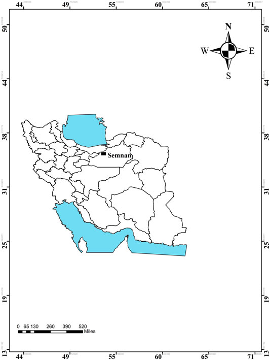
Semnan city, the capital of Semnan Province and Semnan County, is one of the cities of Iran, which is located in the south of the Alborz mountain range and the north of the Kavir plain on Tehran-to-Khorasan road. This city is located at 216 km from Tehran between Damghan and Garmsar cities at 53° 23′ east longitude and 35° 34′ north latitude, with an average altitude of 1,130 m above sea level. The climate of this city is hot in summer and cold in winter. The rainfall of this city is mostly in the cold seasons of the year, and its average annual rainfall is 140 mm. The average annual temperature is 17.01°C, while the maximum, absolute temperature is 43.5°C and the absolute minimum is −8.4°C. The synoptic meteorological station of Semnan city was established in 1965. This station is located at 53° 23′ east longitude and 35° 34’ north latitude, with an altitude of 1,130.8 m above sea level. The climatic identities and statistical yearbooks of the province are used to derive statistical information of the station. Figure 1 illustrates the location of the meteorological station in Semnan city. Given the geographical location and the completeness of the measured information, data related to precipitation in Semnan city were used, which are taken from rainfall statistics from 1973 to 2020 and recorded in the synoptic meteorological station of Semnan city. Statistical data of annual rainfall are given in Table 1.

FIGURE 1

FIGURE 1. Location of Semnan synoptic meteorological station.

TABLE 1

TABLE 1. Statistical data of annual rainfall time series (1973–2020).

Standardized Precipitation Index

To study meteorological drought, various indicators have been developed. One of the most famous indicators is the Standardized Precipitation Index (SPI), which was introduced in 1993 by McKee et al. from the Colorado Climate Center, regarding different effects of rainfall shortage on groundwater, reserves, and surface water resources, soil moisture, and canal flow. This index is obtained based on the difference of precipitation (P) from the average for a specific time scale ($\overline{P}$) and then dividing it by the standard deviation (Sd) ($\text{SPI}=\frac{P-\overline{P}}{Sd}$). Indeed, precipitation is the only effective factor in calculating the Standardized Precipitation Index.

In calculating this index, first the appropriate statistical distribution should be fitted to long-term precipitation data and then the cumulative distribution function should be converted to the normal distribution using equal probabilities. Experience has shown that the precipitation probability distribution often follows the gamma probability distribution. The density function of the gamma distribution probability is as follows:

$\mathrm{f}\left(\mathrm{x}\right)=\frac{1}{{\mathrm{\beta }}^{\mathrm{\alpha }}\mathrm{\Gamma }\left(\mathrm{\alpha }\right)}{\mathrm{x}}^{\mathrm{\alpha }-1}{\mathrm{e}}^{-\frac{\mathrm{x}}{\mathrm{\beta }}},(1)$

where α > 0 is the shape parameter, β > 0 is the scale parameter, x > 0 is the amount of precipitation, and Γ(α) is the gamma function as follows:

$\mathrm{\Gamma }\left(\mathrm{\alpha }\right)={\displaystyle {\int }_0^{\mathrm{\infty }}{\mathrm{y}}^{\mathrm{\alpha }-1}}{\mathrm{e}}^{-\mathrm{y}}\mathrm{d}\mathrm{y}.(2)$

To fit the distribution parameters, α and β are estimated from the sample data:

$\mathrm{\alpha }=\frac{1}{4\mathrm{A}}\left[1+\sqrt{1+\frac{4\mathrm{A}}{3}}\right],(3)$

$\mathrm{\beta }=\frac{\overline{\mathrm{x}}}{\mathrm{\alpha }},(4)$

where $\overline{\mathrm{x}}$ is the mean precipitation and A is given by

$\mathrm{A}=\ln \left(\overline{\mathrm{x}}\right)-\frac{{\displaystyle \sum \ln \left(\mathrm{x}\right)}}{\mathrm{N}}.(5)$

For a given month and time scale, the cumulative probability G(x) of an observed amount of precipitation is given by

$\mathrm{G}\left(\mathrm{x}\right)={\displaystyle {\int }_0^{\mathrm{\infty }}\mathrm{f}\left(\mathrm{x}\right)\mathrm{d}\mathrm{x}}=\frac{1}{{\mathrm{\beta }}^{\mathrm{\alpha }}\mathrm{\Gamma }\left(\mathrm{\alpha }\right)}{\displaystyle {\int }_0^{\mathrm{\infty }}{\mathrm{x}}^{\mathrm{\alpha }-1}{\mathrm{e}}^{-\frac{\mathrm{x}}{\mathrm{\beta }}}\mathrm{d}\mathrm{x}}.(6)$

Since the gamma function is not defined for x = 0 and the rainfall data always contain a large number of observations with zero rainfall, the cumulative probability of rainfall is calculated as follows:

$\mathrm{H}\left(\mathrm{x}\right)=\mathrm{q}+\left(1-\mathrm{q}\right)\mathrm{G}\left(\mathrm{x}\right),(7)$

where q is the probability of zero rainfall in the data series, which is obtained by dividing the number of zero data by the total number of data. By calculating the cumulative probability of rainfall and using Equations 8–11, a normal distribution (Z) with a mean of zero and a standard deviation of one will be obtained.

$\mathrm{Z}=\mathrm{S}\mathrm{P}\mathrm{I}=-\left[\mathrm{t}-\frac{{\mathrm{C}}_0+{\mathrm{C}}_1\mathrm{t}+{\mathrm{C}}_2\mathrm{t}}{1+{\mathrm{d}}_1\mathrm{t}+{\mathrm{d}}_2{\mathrm{t}}^2+{\mathrm{d}}_3{\mathrm{t}}^3}\right]0<\mathrm{H}\left(\mathrm{x}\right)\le 0.5,(8)$

$\mathrm{Z}=\mathrm{S}\mathrm{P}\mathrm{I}=+\left[\mathrm{t}-\frac{{\mathrm{C}}_0+{\mathrm{C}}_1\mathrm{t}+{\mathrm{C}}_2\mathrm{t}}{1+{\mathrm{d}}_1\mathrm{t}+{\mathrm{d}}_2{\mathrm{t}}^2+{\mathrm{d}}_3{\mathrm{t}}^3}\right]0.5<\mathrm{H}\left(\mathrm{x}\right)<1,(9)$

$\mathrm{t}=\sqrt{\ln \left(\frac{1}{\mathrm{H}{\left(\mathrm{x}\right)}^2}\right)},0<\mathrm{H}\left(\mathrm{x}\right)\le 0.5,(10)$

$\mathrm{t}=\sqrt{\ln \left(\frac{1}{{\left(1-\mathrm{H}\left(\mathrm{x}\right)\right)}^2}\right)},0.5<\mathrm{H}\left(\mathrm{x}\right)\le 1,(11)$

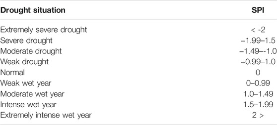
where C₀, C₁, C₂, d₁, d₂, and d₃ have constant coefficients of C₀ = 2.5165, C₁ = 0.8029, C₂ = 0.0103, d ₁ = 1.4328, d₂ = 0.1893, and d₃ = 0.0013, respectively. Thus, the normalized SPI is converted to a normal Z, which reflects the amount of deviations above or below the mean. This index can be computed in short-term (1, 3, 6, and 9 months) and long-term (12, 24, 48, and 72 months) time scales. Drought index with different time scales has been used in various articles and research studies (Hosseini-Moghari and Araghinejad, 2015; Tan et al., 2015; Lee et al., 2017; Spinoni et al., 2017; Brito et al., 2018; Pramudya and Onishi, 2018; Diani et al., 2019; Mahmoudi et al., 2019). After having extracted rainfall data in different monthly or annual scales, a data homogeneity test is carried out and a time series is formed in the mentioned scales. Then, the cumulative probability of cumulative precipitation values is computed at each time scale using the gamma distribution. These values are converted to a normal standard random variable with a zero mean and a variance of one, which is the SPI value. Table 2 presents different classes of drought in this index.

TABLE 2

TABLE 2. Classification of Standardized Precipitation Index assessment.

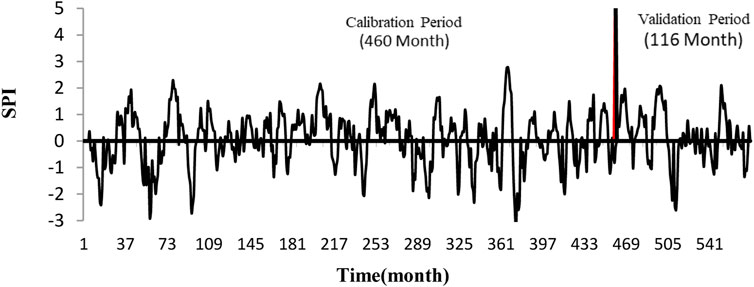
To determine the onset, end, and severity of drought from the SPI drought index according to the classifications presented in Table 2, SPI less than −1 indicates the beginning of a drought, which continues as long as this index is less than −1. On the other hand, SPI greater than 1 represents the beginning of a wet year period. The advantages of SPI include ease of computation, multipurposity to monitor drought conditions from meteorological and hydrological points of view, normal distribution, flexibility to different time scales, independence from soil moisture, and the possibility of use in all months of a year (Hejazizadeh and Javizadeh, 2010). This index has been used in several studies (Sobral et al., 2018; Tirivarombo et al., 2018; Marini et al., 2019; Wang et al., 2019; Zhang et al., 2019; Azimi and Moghaddam, 2020; Bhunia et al., 2020; Bong and Richard, 2020; Li et al., 2020; Won et al., 2020). The present study seeks to first compute the monthly drought index by using the abovementioned method for 576 steps, among which 460 initial data, which are equivalent to 80% of the data, are used for calibration and 116 final data are used to validate the time series model. Figure 2 shows the time series diagram of the SPI drought index (one month) in Semnan.

FIGURE 2

FIGURE 2. Time series of one-month SPI drought index in Semnan.

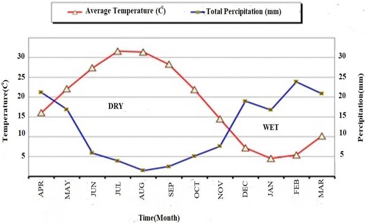
Generally, it is possible to use a moving average for determining the drought index and selecting wet and drought periods such that the correct selection of the time base allows specifying wet and drought periods better. Hence, in addition to raw statistics of SPI data, this study evaluates SPI statistics computed from 6-month rainfall data to predict the time series of the drought index. Figure 3 provides the 6-month SPI time series discussed in this research. The six-month time scale for long-term forecasting of the drought is selected based on the fact that rainfall occurs in Semnan in cold seasons similar to most parts of the country, thus addressing the ombrothermic diagram of Semnan synoptic station (Figure 4).

FIGURE 3

FIGURE 3. Semnan 6-month drought index time series.

FIGURE 4

FIGURE 4. Ombrothermic curve of Semnan synoptic station (during the statistical period).

Time Series Stationarity

If the mean, variance, and covariance are constant in a time series over certain periods (Equations 12–15), the time series is static. On the other hand, the time series will be strictly static if the joint distribution of $x\left(t_1\right)$ to $x\left(t_n\right)$ is similar to the joint distribution of $x(t_1+h)$ to $x(t_n+h)$ for time points of $t_1$ to $t_k$ at any time delay h [8]. In other words, the basic concept of stationarity is that the probabilistic rules governing the process do not change over time and, therefore, the process remains in statistical equilibrium (Johnson et al., 1977).

$\text{E}\left({\left|\text{x}\left(\text{t}\right)\right|}^2\right)<\mathrm{\infty },\text{t}\in \text{Z}(12)$

$\text{E}\left(\text{x}\left(\text{t}\right)\right)={\text{m}}_1,\text{t}\in \text{Z}(13)$

$\text{Var}\left(\text{x}\left(\text{t}\right)\right)={\text{m}}_2,\text{t}\in \text{Z}(14)$

${\text{γ}}_{\text{s}}\left(\text{ r},\text{s }\right)={\text{γ}}_{\text{s}}\left(\text{r}+\text{t},\text{s}+\text{t}\right),\left\{\text{r},\text{s},\text{t}\right\}\in \text{Z}(15)$

where x(t) represents time series, E and Var indicate the mathematical expectation and variance functions, ${\text{γ}}_{\text{s}}$ shows the time series autocovariance function, and ${\text{m}}_1$ and ${\text{m}}_2$ are constant numbers.

The existence of a trend in data is one of the main causes of stationarity. Most climatic and hydrological parameters are seasonal, and the seasonal fluctuations complicate the trend. For this purpose, the seasonal Mann–Kendall test (Equations 16–20) was used to determine the trend in the data.

${\text{S}}^{\text{′}}={\displaystyle \sum }_{\text{j}=1}^{\text{p}}{\text{S}}_{\text{j}}(16)$

where P demonstrates the total number of seasons and Kendall statistics is related to season j ($\text{j}=\mathrm{1,2},\dots ,\text{ p}$) and computed according to

${\text{S}}_{\text{j}}={\displaystyle \sum }_{\text{i}=1}^{{\text{n}}_{\text{j}}}{\displaystyle \sum }_{\text{k}=\text{i}+1}^{{\text{n}}_{\text{j}}-1}\mathrm{sgn}\left(\text{x}\left(\text{i}\right)-\text{x}\left(\text{k}\right)\right)(17)$

In the absence of sequential correlations in data, the variance is obtained from Eq. 18. If there is a sequential correlation in the time series data, the variance can be computed from Eq. 19:

${\text{σ}}_{{\text{S}}^{\text{'}}}^2={\displaystyle \sum }_{\text{j}=1}^{\text{p}}\text{Var}\left({\text{S}}_{\text{j}}\right)(18)$

${\text{σ}}_{{\text{S}}^{\text{'}}}^2={\displaystyle \sum }_{\text{j}=1}^{\text{p}}\text{Var}\left({\text{S}}_{\text{j}}\right)+{\displaystyle \sum }_{\text{g}=1}^{\text{p}-1}{\displaystyle \sum }_{\text{h}=\text{g}+1}^{\text{p}}{\text{σ}}_{\text{gh}}(19)$

where ${\text{σ}}_{\text{gh}}$ shows the covariance between Kendall statistics in seasons g and h. With the assumption of data independence, it can be assumed that $\text{cov}\left({\text{S}}_{\text{g}},{\text{ S}}_{\text{h}}\right)=0$. Finally, a statistic named $\text{Z'}$ is obtained from the following relationships:

${\text{Z}}^{\text{'}}=\left\{\begin{array}{c}\frac{\text{S′}-1}{{\text{σ}}_{\text{S′}}}\\ 0,\mathrm{S}\prime =0\\ \frac{\text{S′}+1}{{\text{σ}}_{\text{S′}}}\end{array}\right\}(20)$

If the probability value $Z$ computed according to Eq. 20 is less than 5%, it indicates the existence of a trend in the time series.

Since the time series stationarity is a fundamental assumption in modeling and predicting the stationarity, it is possible to use the differencing approach to make series static as much as possible. In this research, an augmented Dickey–Fuller (ADF) test is used to determine how much the mentioned series become static after non-seasonal, seasonal, and combined differencing. This test (Equations 21–24) acts based on the presence or absence of a single root to specify the stationarity of the time series by examining the absence of a single root.

$\text{Δx}\left(\text{t}\right)=\text{α}+{\text{β}}_1\text{t}+{\text{β}}_2{\text{t}}^2+\text{γx}\left(\text{t}-1\right)\pm +{\mathrm{\varphi }}_1\text{Δx}\left(\text{t}-1\right)+\mathrm{...}+{\mathrm{\varphi }}_{\text{p}-1}\text{Δx}\left(\text{t}-\text{p}+1\right)+\text{ε}\left(\text{t}\right)(21)$

$\text{τ}=\frac{\widehat{\text{γ}}}{{\text{σ}}_{\widehat{\text{γ}}}}(22)$

${\text{H}}_0:\text{γ}=0(23)$

${\text{H}}_1:\text{γ}<0(24)$

where $\text{Δ}$ represents the first-order differential operator and $\alpha ,$ ${\beta }_1$, and ${\beta }_2$ indicate a constant value and coefficients of the linear and quadratic trends, respectively. Furthermore, ${\phi }_i$ is the $i$-order autocorrelation coefficient, $p$ is the maximum self-correlation, $\tau$ is the augmented Dickey–Fuller test statistic, $\gamma$ is the estimated coefficient or root, ${\sigma }_{\widehat{\gamma }}$ is the estimated standard error, $H_0$ is the null hypothesis indicating the existence of a single root, and $H_0$ is the alternative hypothesis that implies the lack of existence of a single root.

After computing the parameter $\tau$, if this statistic is less than the critical value in the Dickey–Fuller distribution, the null hypothesis is rejected, meaning that there is no single root and the series is static. Each of the values $\alpha$, ${\beta }_1$, and ${\beta }_2$ can be considered as zero, according to which different states such as without constant and trend state, only constant, constant and linear trend, and the quadratic trend will be tested.

Since the augmented Dickey–Fuller test fails to consider the effect of the periodic component on instationarity of the series, it is necessary to use other tests for seasonal series. In this way, drawing a correlogram and examining it intuitively is one of the methods to retest the stationarity. This diagram shows the values of autocorrelation function (ACF) for different time steps. If the time series is static, this diagram will damp to zero exponentially or oscillating [9]. In this diagram, the value of data autocorrelation coefficient ($\rho$) will be plotted for different steps. The value of autocorrelation coefficient for step h is obtained from

$\rho \left(h\right)=\frac{{{\displaystyle \sum }}_{t=h}^n\left(x\left(t\right)-\overline{x}\right)\left(x(t-h)-\overline{x}\right)}{{{\displaystyle \sum }}_{t=h}^n{\left(x\left(t\right)-\overline{x}\right)}^2}h=\mathrm{1,2},,\mathrm{...},n/4.(25)$

Time Series Models

Given the existence of different time series models based on Box–Jenkins theories, this research utilizes ARIMA models and their general form, multiplicative seasonal ARIMA, to predict the drought index. The multiplicative seasonal ARIMA model is presented with the following relationships (Salas et al., 1980):

$\text{SARIMA}\left(\text{p},\text{d},\text{q}\right)\left(\text{P},\text{D},\text{Q}\right):\text{Φ}\left({\text{B}}^{\text{ω}}\right)\text{φ}\left(\text{B}\right){\left(1-{\text{B}}^{\text{ω}}\right)}^{\text{D}}{\left(1-\text{B}\right)}^{\text{d}}\text{x}\left(\text{t}\right)=\text{Θ}\left({\text{B}}^{\text{ω}}\right)\text{θ}\left(\text{B}\right)\text{ε}\left(\text{t}\right)(26)$

$\text{Φ}\left({\text{B}}^{\text{ω}}\right)=\left(1-{\text{Φ}}_1{\text{B}}^{\text{ω}}-{\text{Φ}}_2{\text{B}}^{2\text{ω}}-\mathrm{...}-{\text{Φ}}_{\text{P}}{\text{B}}^{\text{Pω}}\right)(27)$

$\varphi \left(\text{B}\right)=\left(1-{\varphi }_1\text{B}-{\varphi }_2{\text{B}}^2-\mathrm{...}-{\varphi }_{\text{P}}{\text{B}}^{\text{P}}\right)(28)$

$\text{Θ}\left({\text{B}}^{\text{ω}}\right)=\left(1-{\text{Θ}}_1{\text{B}}^{\text{ω}}-{\text{Θ}}_2{\text{B}}^{2\text{ω}}-\mathrm{...}-{\text{Θ}}_{\text{Q}}{\text{B}}^{\text{Qω}}\right)(29)$

$\text{θ}\left(\text{B}\right)=\left(1-{\text{θ}}_1\text{B}-{\text{θ}}_2{\text{B}}^2-\mathrm{...}-{\text{θ}}_{\text{q}}{\text{B}}^{\text{q}}\right)(30)$

where $x\left(t\right)$: drought index time series, $\epsilon \left(t\right)$: residual series, $p$: non-seasonal autocorrelation parameter order, $q$: non-seasonal moving average parameter order, $P$: seasonal autocorrelation parameter order, $Q$: seasonal moving average parameter order, $\omega$: period, $\phi$: non-seasonal autocorrelation parameter, $\theta$: seasonal moving average parameter, $\text{Φ}$: seasonal autocorrelation parameter, $\text{Θ}$: seasonal moving average parameter, $B$: differential operator, ${(1-B^{\omega })}^D$: $D$-th seasonal differencing by step $\omega$, and ${(1-B)}^d$: $d$-th non-seasonal differencing operation.

The maximum order of parameters of the mentioned models in the relations (26) to (30) ($p, q, P, Q$) can be identified from the ACF diagram. If the orders required for parameters of each model are $p=\{\mathrm{0,1},\mathrm{....},l\}$, $q=\{\mathrm{0,1},\mathrm{....},m\}$, $P=\{\mathrm{0,1},\mathrm{....},n\}$, and $Q=\{\mathrm{0,1},\mathrm{....},o\}$, then the number of required models (NOM) is obtained according to the probability rule and based on

${\text{NOM}}_{\text{SARIMA}}=\left(\text{l}+1\right)\left(\text{m}+1\right)\left(\text{n}+1\right)\left(\text{o}+1\right)(31)$

Models Assessment Criteria

To achieve the most accurate model, valid assessment criteria are fitted on the desired time series. In this study, criteria of correlation coefficient (R), root mean square error (RMSE), and mean absolute error (MAE) are used to evaluate and analyze the model results. These criteria are shown as follows:

$\text{R}=\frac{{{\displaystyle \sum }}_{\text{i}=1}^{\text{n}}\left({\text{x}}_{\text{i}}^{\text{o}}-{\overline{\text{x}}}^{\text{o}}\right)\left({\text{x}}_{\text{i}}^{\text{p}}-{\overline{\text{x}}}^{\text{p}}\right)}{\sqrt{{{\displaystyle \sum }}_{\text{i}=1}^{\text{n}}{\left({\text{x}}_{\text{i}}^{\text{o}}-{\overline{\text{x}}}^{\text{o}}\right)}^2{{\displaystyle \sum }}_{\text{i}=1}^{\text{n}}{\left({\text{x}}_{\text{i}}^{\text{p}}-{\overline{\text{x}}}^{\text{p}}\right)}^2}}(32)$

$\text{RMSE}=\sqrt{\frac{1}{\text{n}}{\displaystyle \sum }_{\text{i}=1}^{\text{n}}{\left({\text{x}}_{\text{i}}^{\text{p}}-{\text{x}}_{\text{i}}^0\right)}^2}(33)$

$\text{MAE}=\frac{1}{\text{n}}{\displaystyle \sum }_{\text{i}=1}^{\text{n}}\left|\left({\text{x}}_{\text{i}}^0-{\text{x}}_{\text{i}}^{\text{p}}\right)\right|(34)$

where $x_i^o$ represents the observational values, $x_i^p$ indicates the predicted values, ${\overline{x}}^{\text{o}}$ shows the mean observational values, and ${\overline{x}}^p$ is the mean predicted values. Based on the results, it can be said that the closer the RMSE and MAE values are to zero, the better the performance of the model will be. The value of the correlation coefficient, which varies between −1 and 1, is close to zero in a superior case.

After reviewing assessment criteria and selecting the best model, the suitability of residues from the results is examined and if approved, the model is selected. Finally, using the selected model, the drought index parameter can be predicted in future.

Evaluating the Independence of Residuals

If a time series model is correctly specified, then the residues obtained from the model fitting should approximately have the characteristics of independent normal random variables with a zero mean and a constant variance. In this study, the rest of the selected fitted model is examined and analyzed to ensure its accuracy. To this aim, the diagrams of the normal probability of residuals, residuals versus fitted values, residuals over time, residual histograms, and residual autocorrelation and partial autocorrelation functions are plotted and interpreted. If the selected model is identified correctly, it has signs among the abovementioned diagrams. If the residuals are along a straight line in the normal probability diagram, it indicates the normality of residuals. If the residuals are around the zero horizontal plane with a trendless rectangular scattering in the residual over time diagram, have no structure in the residuals versus fits and residual versus order plots, and have no special trend in ACF and PACF diagrams and do not exceed its permissible limits, it is possible to accept the constantness of variance and randomness and independency of the residuals, respectively.

In addition to graph methods, the Portmanteau test is used to examine the suitability of the model. This test uses residual autocorrelation to test the null hypothesis ($H_0$), i.e., the lack of any correlation between model residues, using test statistics $Q$. If the value of statistic Q is greater than the corresponding value of the chi-square probability table (${\chi }^2$), the hypothesis ($H_0$), which is sometimes called the model adequacy hypothesis, is rejected. It should be noted that the probabilistic values corresponding to this test (p value) are evaluated for the confidence level of 95% by assuming the independence of residuals.

Results and Discussion

This research seeks to study and compute two time series, one related to SPI monthly drought index data and the other related to six-month data of the SPI parameter, along with different differencing time series.

The drought index has different time divisions, and for some reason, one-month and six-month drought indexes are mostly used in resources. The one-month SPI is a short-term drought index and can be a better indicator of monthly percipitation for a given region compared to other time steps. The 6-month SPI shows medium-term percipitation trends and can be used to represent percipitation in different seasons much more effectively. The resulting information may also be related to abnormal flows and water reservoir levels. Before modeling the drought index time series, time series stationarity is examined using the seasonal Kendall test whose results are shown in Table 3. According to coefficients obtained for each of the series, the seasonal Mann–Kendall test reveals that both time series are static. Furthermore, different types of non-seasonal (d = 1), seasonal (D = 1), and combined (d = 1, D = 1) differencing are performed on both time series, resulting in forming new time series. The role of different differencing operations in the time series stationarity is determined by using the augmented Dickey–Fuller (ADF) test. Results of the augmented Dickey–Fuller test for drought index time series are provided in Table 4. According to the results, it is observed how differencing operation leads to better stationarity of time series. Consequently, combined differencing shows the highest degree of stationarity compared to other cases.

TABLE 3

TABLE 3. Results of evaluating time series with the seasonal Mann–Kendall test.

TABLE 4

TABLE 4. Results of the augmented Dickey–Fuller test for drought index time series.

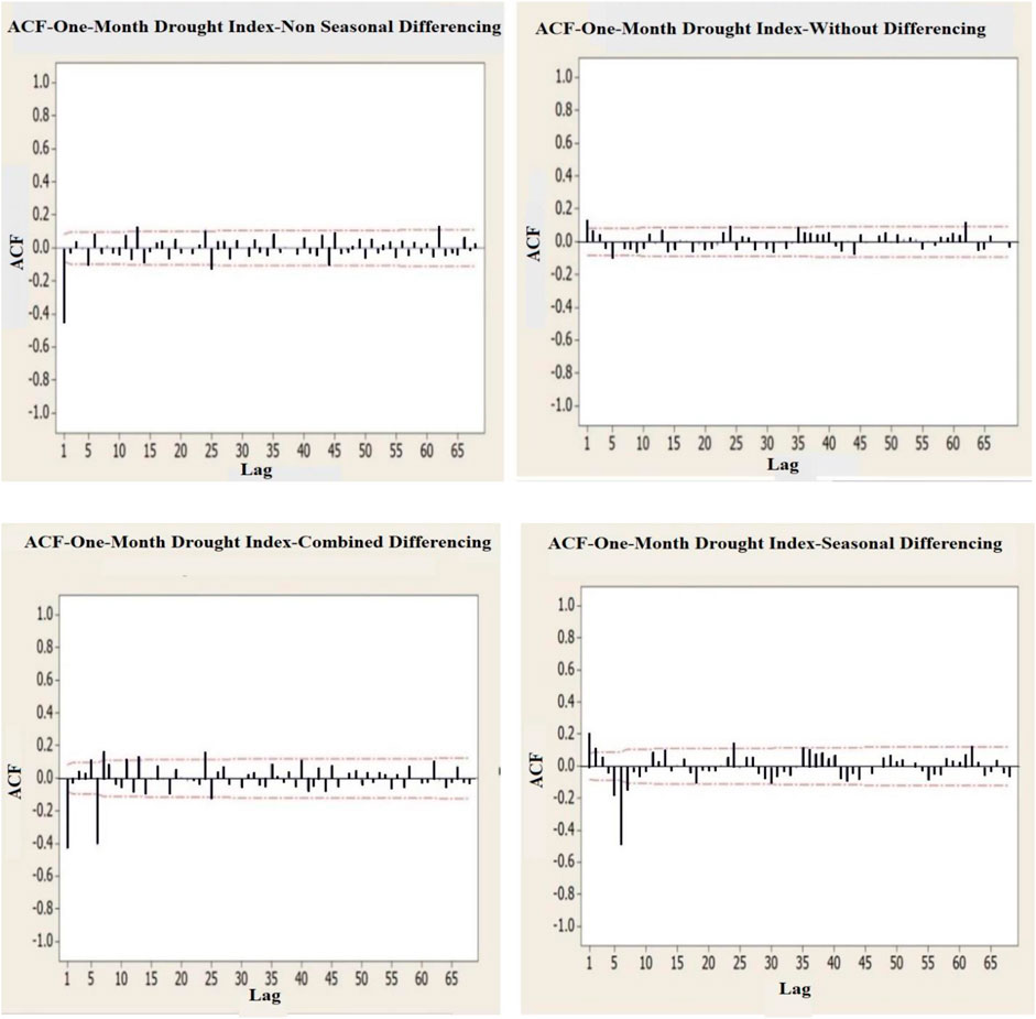
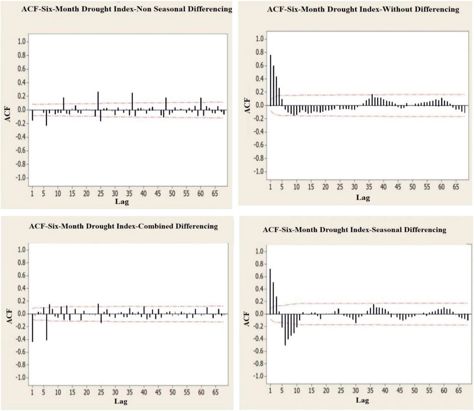
However, the Dickey–Fuller test sometimes presents a poor performance in determining the stationarity of seasonal series. Furthermore, no information is available on the exact seasonality of differenced data for the series studied in this research. Further validation is performed by drawing autocorrelation diagrams and the stationarity of different types of series without differencing and with non-seasonal, seasonal, and combined differencing is investigated with results as shown in Figures 5, 6. As observed, none of the series is undamped and oscillating and has no periodicity, and consequently, all series approach zero after a few steps and are within the 95% confidence level, confirming the stationarity of the series.

FIGURE 5

FIGURE 5. Autocorrelation diagrams of different states of one-month drought index time series.

FIGURE 6

FIGURE 6. Autocorrelation diagrams of different states of six-month drought index time series.

By using correlogram diagrams (ACF and PACF diagrams), it is possible to determine the maximum number of parameters required for time series models, in addition to stationarity. This number, which is obtained based on steps with large values from this diagram, along with the number of models required to achieve the most accurate model is presented in Tables 5, 6.

TABLE 5

TABLE 5. Orders of parameter and number of models required for the six-month drought index.

TABLE 6

TABLE 6. Orders of parameter and number of models required for the one-month drought index.

Another issue that can be deduced from Figures 6, 7 and Tables 5, 6 is the type of model suitable for modeling and forecasting. Therefore, by placing different orders of P, Q, p, and q, time series are modeled by different states and then predicted and evaluated in the validation period.

FIGURE 7

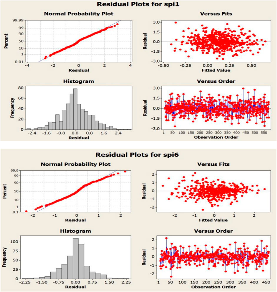
FIGURE 7. Analysis diagrams of the residual of the selected model for one- and six-month drought index time series.

Tables 7, 8 report the most accurate models, along with the results of their assessment criteria, for both the calibration and validation periods for one- and six-month drought index time series. Accordingly, the seasonal SARIMA (202) (111)₆ model is introduced as the selected model of one-month drought index, while the seasonal SARIMA (503) (111)₆ model is chosen as the selected model for the six-month drought index. Furthermore, the results reveal that the ratio of increasing the accuracy of forecasting the six-month drought index is highly significant compared to the one-month drought index. It is also worth mentioning that the comparison of drought index time series modeling in the study area with other artificial intelligence methods, such as the neural network or adaptive neuro-fuzzy inference system, has already been performed to show the superiority of the selected time series models in this field (Sadeghian et al., 2020).

TABLE 7

TABLE 7. Results of evaluating the best models in differencing states for the six-month drought index.

TABLE 8

TABLE 8. Results of evaluating the best models in differencing states for the one-month drought index.

Evaluating Model Adequacy

To ensure the accuracy of the selected model, residuals of the fitted model are analyzed. For this purpose, the Portmanteau test is conducted for each selected model, and then, various diagrams related to residuals are examined. Table 9 provides the results of the Portmanteau test.

TABLE 9

TABLE 9. Results of the Portmanteau test for the selected one- and six-month drought index models.

As observed, the p value for delays is greater than 0.05 even up to step 24, enabling us to accept the assumption that all autocorrelations are zero. Additionally, the graphs obtained from residuals of the models mentioned in Figures 7, 8 indicate the suitability and adequacy of the models. Figure 7 shows the analysis diagrams of the residual of the selected model for one- and six-month drought index time series (SP1-1 and SPI-6). Figure 8 shows the ACF and PACF diagrams of residual of the selected model for one- and six-month drought index time series.

FIGURE 8

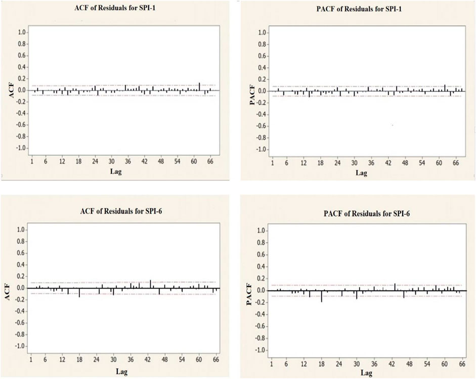
FIGURE 8. ACF and PACF diagrams of residual of the selected model for one- and six-month drought index time series.

Forecasting

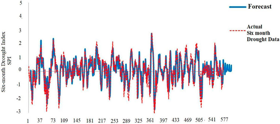
After reviewing the different models and reaching the best selected model, the six-month model with the SARIMA format (3,0,5) (1,1,1) and the resulting values of the model along with the drought index values that occurred in reality were plotted. As shown in Figure 9, the results of the model are in good agreement with the real situation which the numerical indices of Table 7 had previously emphasized.

FIGURE 9

FIGURE 9. Diagram of the selected model for forecasting drought index data.

By selecting the best proposed model, SARIMA (3,0,5) (1,1,1)₆, for the six-month drought index and addressing Eqs 26–30, the six-month drought index model is obtained according to

$\left(1+0.349{\text{B}}^6\right)\left(1-0.561\text{B}-0.627{\text{B}}^2-0.305{\text{B}}^3+0.552{\text{B}}^4+0.026{\text{B}}^5\right)\left(1-{\text{B}}^6\right)\text{X}\left(\text{t}\right)=\left(1-0.979{\text{B}}^6\right)\left(1+0.231\text{B}-0.342{\text{B}}^2-0.607{\text{B}}^3\right)\text{ε}\left(\text{t}\right),(35)$

where $B$ represents the differential operator and $\text{x}\left(\text{t}\right)$ and $\text{ε}\left(\text{t}\right)$ are the drought index and residual series, respectively. In order to have a vision of the future, the selected model was used to evaluate the situation for the next 24 months. Applying Eq. 35 to the actual data of the six-month time series of the SPI drought index for 24 months creates a predicted series which is marked with a blue line in Figure 9.

Comparison Between Observed and Predicted Drought Characteristics

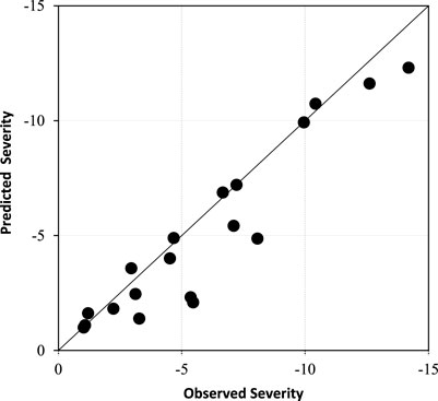
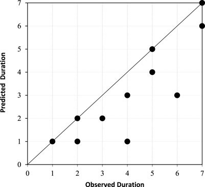
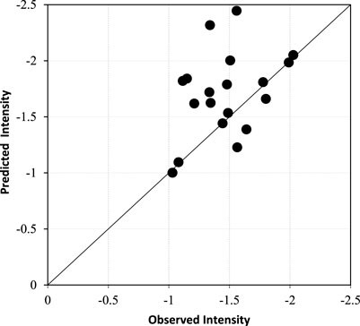
After modeling with the best proposed model and comparing the results of the drought index between the model and the observed data, the severity, duration, and intensity of the drought (SPI < −1) were also examined. Accordingly, the graphs in Figures 10–12 show the comparison between severity, duration, and intensity of the SPI during droughts, respectively. As can be seen in these figures, there is a good agreement in the direction of the 45-degree axis between the points, which indicates the superiority of the proposed model.

FIGURE 10

FIGURE 10. Comparison between observed and predicted drought severity.

FIGURE 11

FIGURE 11. Comparison between observed and predicted drought duration.

FIGURE 12

FIGURE 12. Comparison between observed and predicted drought intensity.

Conclusion

Predicting hydrological variables, especially the drought index, has long been considered by many researchers, and various research studies have been conducted on this field, due to the importance and widespread use of the SPI in topics such as climate change and meteorology. The present study addresses the initial stationarity of drought index time series taken from rainfall statistics of Semnan meteorological station and then evaluates the effect of different non-seasonal, seasonal, and combined differencing on the time series stationarity, as well as the results of their selected models. For innovation in the research, we analyze the degree of increase in forecast accuracy and the effect of differencing operators on six-month drought index time series. The major findings can be summarized as follows. 1. Although both one- and six-month drought index time series are static, different differencing operations improve their static degree so that series with the combined differencing operator (non-seasonal and seasonal) provide the best stationarity degree based on the results of the augmented Dickey–Fuller test. 2. Given the results of the ombrothermic curve and according to the precipitation conditions of the region, the seasonal period for modeling the drought index is considered 6 months. The best models from one- and six-month drought index time series are originated from seasonal differencing. Accordingly, SARIMA (2,0,2) (1,1,1)₆ and SARIMA (3,0,5) (1,1,1)₆ are the selected models for one- and six-month drought index time series, respectively. 3. The results indicate that the accuracy of models in calibration is significantly higher than that of validation for both selected series models resulting from seasonal differencing of one- and six-month drought index. Moreover, the six-month drought index has better modeling than the one-month drought index for both models. 4. For the selected time series model of one-month drought index SARIMA (2,0,2) (1,1,1), the results of RMSE, MAE, and R assessment criteria equal to 0.752, 0.510, and 0.218 in the calibration stage and 0.823, 0.589, and 0.039 in the validation stage, indicating poor performance of the time series in modeling and predicting the one-month drought index variable. 5. For the SARIMA (3,0,5) (1,1,1) model, the results of RMSE, MAE, and R equal to 0.58, 0.430, and 0.812 in the calibration stage and 910, 0.689, and 0.341 in the validation stage, respectively, highlighting a significant improvement (about 4 times increase in correlation coefficient in the calibration stage and 8 times in the validation stage) compared to the one-month drought index. Also, the severity, duration, and intensity of the drought of the selected model and observed data were compared, and the results indicated a good agreement. The results of the present study have the potential to be used for similar regions in future research.

Data Availability Statement

The original contributions presented in the study are included in the article/Supplementary Material, further inquiries can be directed to the corresponding authors.

Author Contributions

• Conceptualization: SB, Y-WJ, AM, and K-WC. • Data curation: HK, SB, SF, MM, and SB. • Formal analysis: SF, SB, and HK. • Investigation: HK, SB, Y-WJ, AM, MM, K-WC, and SB. • Methodology: HK, SB, Y-WJ, SF, MM, SB, and SB. • Resources: HK, SF, MM, SB, and SB. • Software: SF, MM, SB, AM, and K-WC. • Supervision: SB and HK. • Validation: SB, HK, Y-WJ, SF, MM, K-WC, and SB. • Visualization: SB and HK. • Writing–original draft: HK, SF, MM, SB, and SB. • Writing–review and editing: HK, Y-WJ, SF, MM, SB, AM, and K-WC.

Conflict of Interest

The authors declare that the research was conducted in the absence of any commercial or financial relationships that could be construed as a potential conflict of interest.

Publisher’s Note

All claims expressed in this article are solely those of the authors and do not necessarily represent those of their affiliated organizations, or those of the publisher, the editors, and the reviewers. Any product that may be evaluated in this article, or claim that may be made by its manufacturer, is not guaranteed or endorsed by the publisher.

References

Azimi, S., and Moghaddam, M. A. (2020). Modeling Short Term Rainfall Forecast Using Neural Networks, and Gaussian Process Classification Based on the SPI Drought Index. Water Resour. Manage. 34 (4), 1–37. doi:10.1007/s11269-020-02507-6

CrossRef Full Text | Google Scholar

Bahrami, M., Bazrkar, S., and Zarei, A. R. (2019). Modeling, Prediction and Trend Assessment of Drought in Iran Using Standardized Precipitation index. J. Water Clim. Change 10 (1), 181–196. doi:10.2166/wcc.2018.174

CrossRef Full Text | Google Scholar

Barua, S., Ng, A. W. M., and Perera, B. J. C. (2012). Artificial Neural Network-Based Drought Forecasting Using a Nonlinear Aggregated Drought Index. J. Hydrol. Eng. 17, 1408–1413. doi:10.1061/(asce)he.1943-5584.0000574

CrossRef Full Text | Google Scholar

Bhunia, P., Das, P., and Maiti, R. (2020). Meteorological Drought Study through SPI in Three Drought Prone Districts of West Bengal, India. Earth Syst. Environ. 4 (1), 43–55. doi:10.1007/s41748-019-00137-6

CrossRef Full Text | Google Scholar

Bong, C. H. J., and Richard, J. (2020). Drought and Climate Change Assessment Using Standardized Precipitation index (SPI) for Sarawak River Basin. J. Water Clim. Change 11 (4), 956–965. doi:10.2166/wcc.2019.036

CrossRef Full Text | Google Scholar

Brito, S. S. B., Cunha, A. P. M. A., Cunningham, C. C., Alvalá, R. C., Marengo, J. A., and Carvalho, M. A. (2018). Frequency, Duration and Severity of Drought in the Semiarid Northeast Brazil Region. Int. J. Climatol 38 (2), 517–529. doi:10.1002/joc.5225

CrossRef Full Text | Google Scholar

Cryer, J. D., and Chan, K. S. (2008). Time Series Analysis with Applications in R. Second Ed. NY: Springer.

Google Scholar

Danandeh Mehr, A., Vaheddoost, B., and Mohammadi, B. (2020). ENN-SA: A Novel Neuro-Annealing Model for Multi-Station Drought Prediction. Comput. Geosciences 145, 104622. doi:10.1016/j.cageo.2020.104622

CrossRef Full Text | Google Scholar

Diani, K., Kacimi, I., Zemzami, M., Tabyaoui, H., and Haghighi, A. T. (2019). Evaluation of Meteorological Drought Using the Standardized Precipitation Index (SPI) in the High Ziz River Basin, Morocco. Limnol. Rev. 19 (3), 125–135. doi:10.2478/limre-2019-0011

CrossRef Full Text | Google Scholar

Hejazizadeh, Z., and Javizadeh, S. (2010). Introduction to Drought and its Indices. SMT Incorporated.

Google Scholar

Hosseini-Moghari, S. M., and Araghinejad, S. (2015). Monthly and Seasonal Drought Forecasting Using Statistical Neural Networks. Environ. Earth Sci. 74 (1), 397–412. doi:10.1007/s12665-015-4047-x

CrossRef Full Text | Google Scholar

Jalili, M., Gharibshah, J., Ghavami, S. M., Beheshtifar, M. R., and Farshi, R. (2013). Nationwide Prediction of Drought Conditions in Iran Based on Remote Sensing Data. IEEE Trans. Comput. 63 (1), 90–101. doi:10.1109/TC.2013.118

CrossRef Full Text | Google Scholar

Johnson, D. E., Bhattacharyya, G. K., Johnson, R. A., and Bhattacharyya, G. (1977). Statistical Concepts and Methods. John Wiley & Sons Incorporated, 106.

Google Scholar

Karamouz, M., and Araghinejad, S. (2010). Advanced Hydrology. Tehran, Iran: Industrial University of Amir Kabir Poly Technics.

Google Scholar

Karimi, M., Melesse, A. M., Khosravi, K., Mamuye, M., and Zhang, J. (2019). “Analysis and Prediction of Meteorological Drought Using SPI index and ARIMA Model in the Karkheh River Basin, Iran,” in Extreme Hydrology and Climate Variability (Karkheh River basin, Iran: Elsevier), 343–353. doi:10.1016/b978-0-12-815998-9.00026-9

CrossRef Full Text | Google Scholar

Komasi, M., Alami, M. T., and Nourani, V. (2013). Drought Forecasting by SPI Index and ANFIS Model Using Fuzzy C-Mean Clustering. J. Water Wastewater 24 (4), 90–102. Available at http://www.wwjournal.ir/article_3196.html?lang=en.

Google Scholar

Lee, S.-H., Yoo, S.-H., Choi, J.-Y., and Bae, S. (2017). Assessment of the Impact of Climate Change on Drought Characteristics in the Hwanghae Plain, North Korea Using Time Series SPI and SPEI: 1981-2100. Water 9 (8), 579. doi:10.3390/w9080579

CrossRef Full Text | Google Scholar

Li, L., She, D., Zheng, H., Lin, P., and Yang, Z.-L. (2020). Elucidating Diverse Drought Characteristics from Two Meteorological Drought Indices (SPI and SPEI) in China. J. Hydrometeorology 21 (7), 1513–1530. doi:10.1175/jhm-d-19-0290.1

CrossRef Full Text | Google Scholar

Mahmoudi, P., Rigi, A., and Kamak, M. M. (2019). Evaluating the Sensitivity of Precipitation-Based Drought Indices to Different Lengths of Record. J. Hydrol. 579, 124181. doi:10.1016/j.jhydrol.2019.124181

CrossRef Full Text | Google Scholar

Malik, A., and Kumar, A. (2020). Meteorological Drought Prediction Using Heuristic Approaches Based on Effective Drought index: a Case Study in Uttarakhand. Arab J. Geosci. 13, 276. doi:10.1007/s12517-020-5239-6

CrossRef Full Text | Google Scholar

Malik, A., Kumar, A., Salih, S. Q., Kim, S., Kim, N. W., Yaseen, Z. M., et al. (2020). Drought index Prediction Using Advanced Fuzzy Logic Model: Regional Case Study over Kumaon in India. Plos one 15 (5), e0233280. doi:10.1371/journal.pone.0233280

PubMed Abstract | CrossRef Full Text | Google Scholar

Malik, A., Tikhamarine, Y., Sammen, S. S., Abba, S. I., and Shahid, S. (2021a). Prediction of Meteorological Drought by Using Hybrid Support Vector Regression Optimized with HHO Versus PSO Algorithms. Environ. Sci. Pollut. Res. 28, 39139–39158. doi:10.1007/s11356-021-13445-0

CrossRef Full Text | Google Scholar

Malik, A., Tikhamarine, Y., Souag-Gamane, D., Rai, P., Sammen, S. S., and Kisi, O. (2021b). Support Vector Regression Integrated with Novel Meta-Heuristic Algorithms for Meteorological Drought Prediction. Meteorol. Atmos. Phys. 133 (3), 891–909. doi:10.1007/s00703-021-00787-0

CrossRef Full Text | Google Scholar

Marini, G., Fontana, N., and Mishra, A. K. (2019). Investigating Drought in Apulia Region, Italy Using SPI and RDI. Theor. Appl. Climatol 137 (1), 383–397. doi:10.1007/s00704-018-2604-4

CrossRef Full Text | Google Scholar

Montaseri, M., Amirataee, B., and Khalili, K. (2016). Identification of Trend in Spatial and Temporal Dry and Wet Periods in Northwest of Iran Based on SPI and RAI Indices. J. Water Soil 30 (2), 655–671. Available at https://www.cabdirect.org/cabdirect/abstract/20173236578.

Google Scholar

Negaresh, H., and Aramesh, M. (2012). Drought Forecasting in Khash City by Using Neural Network Model. Arid Regions Geogr. Stud. 2 (6), 33–50.

Google Scholar

Niknam, H. H., Moghadam, M. A., and Khosravi, M. (2013). Drought Forecasting Using Adaptive Neuro-Fuzzy Inference Systems (ANFIS), Drought Time Series and Climate Indices for Next Coming Year, (Case Study: Zahedan). Water and Wastewater 2, 42–51. Available at http://www.wwjournal.ir/article_1642.html?lang=en.

Google Scholar

Poornima, S., and Pushpalatha, M. (2019). Drought Prediction Based on SPI and SPEI with Varying Timescales Using LSTM Recurrent Neural Network. Soft Comput. 23 (18), 8399–8412. doi:10.1007/s00500-019-04120-1

CrossRef Full Text | Google Scholar

Pramudya, Y., and Onishi, T. (2018). Assessment of the Standardized Precipitation Index (SPI) in Tegal City, Central Java, Indonesia. IOP Conf. Ser. Earth Environ. Sci. 129 (1), 012019. doi:10.1088/1755-1315/129/1/012019

CrossRef Full Text | Google Scholar

Sadeghian, M., Karami, H., and Mousavi, S. F. (2020). Evaluating the Performance of Time-Series, Neural Network and Neuro-Fuzzy Models in Prediction of Meteorological Drought (Case Study: Semnan Synoptic Station). Irrigation Sci. Eng. 43 (2), 1–18. doi:10.22055/jise.2017.17729.1283

CrossRef Full Text | Google Scholar

Sadeghian, M., Karami, H., and Mousavi, S. F. (2018). Selection of a Proper Model to Predict Monthly Drought in Semnan Using Weather Data and Linear and Nonlinear Models. J. Water Soil Sci. 21 (4), 57–70. doi:10.29252/jstnar.21.4.57

CrossRef Full Text | Google Scholar

Salas, J. D., Delleur, J. W., Yevjevich, V., and Lane, W. L. (1980). Applied Modeling of Hydrologic Time Series. Colorado: Water Resources Publication.

Google Scholar

Shirmohammadi, B., Moradi, H., Moosavi, V., Semiromi, M. T., and Zeinali, A. (2013). Forecasting of Meteorological Drought Using Wavelet-ANFIS Hybrid Model for Different Time Steps (Case Study: Southeastern Part of East Azerbaijan Province, Iran). Nat. Hazards 69, 389–402. doi:10.1007/s11069-013-0716-9

CrossRef Full Text | Google Scholar

Sobhani, B., Safarian Zengir, V., and Kianian, M. K. (2019). Modeling, Monitoring and Prediction of Drought in Iran. Iranian (Iranica) J. Energ. Environ. 10 (3), 216–224. doi:10.5829/IJEE.2019.10.03.09

CrossRef Full Text | Google Scholar

Sobral, B. S., Oliveira-Júnior, J. F., de Gois, G., and Pereira-Júnior, E. R. (2018). Spatial Variability of SPI and RDIstdrought Indices Applied to Intense Episodes of Drought Occurred in Rio de Janeiro State, Brazil. Int. J. Climatol 38 (10), 3896–3916. doi:10.1002/joc.5542

CrossRef Full Text | Google Scholar

Spinoni, J., Naumann, G., and Vogt, J. V. (2017). Pan-European Seasonal Trends and Recent Changes of Drought Frequency and Severity. Glob. Planet. Change 148, 113–130. doi:10.1016/j.gloplacha.2016.11.013

CrossRef Full Text | Google Scholar

Tan, C., Yang, J., and Li, M. (2015). Temporal-Spatial Variation of Drought Indicated by SPI and SPEI in Ningxia Hui Autonomous Region, China. Atmosphere 6 (10), 1399–1421. doi:10.3390/atmos6101399

CrossRef Full Text | Google Scholar

Tirivarombo, S., Osupile, D., and Eliasson, P. (2018). Drought Monitoring and Analysis: Standardised Precipitation Evapotranspiration index (SPEI) and Standardised Precipitation Index (SPI). Phys. Chem. Earth, Parts A/B/C 106, 1–10. doi:10.1016/j.pce.2018.07.001

CrossRef Full Text | Google Scholar

Vaziri, H. R., Karami, H., Mousavi, S. F., and Hadiani, O. (2018). Optimizing Reservoirs Exploitation with a New Crow Search Algorithm Based on a Multi-Criteria Decision-Making Model. J. Water Soil Sci. 22 (1), 279–290. doi:10.29252/jstnar.22.1.279

CrossRef Full Text | Google Scholar

Wang, H., Chen, Y., Pan, Y., Chen, Z., and Ren, Z. (2019). Assessment of Candidate Distributions for SPI/SPEI and Sensitivity of Drought to Climatic Variables in China. Int. J. Climatol 39 (11), 4392–4412. doi:10.1002/joc.6081

CrossRef Full Text | Google Scholar

Won, J., Choi, J., Lee, O., and Kim, S. (2020). Copula-Based Joint Drought Index Using SPI and EDDI and its Application to Climate Change. Sci. Total Environ. 744, 140701. doi:10.1016/j.scitotenv.2020.140701

PubMed Abstract | CrossRef Full Text | Google Scholar

Xu, D., Zhang, Q., Ding, Y., and Huang, H. (2020). Application of a Hybrid ARIMA-SVR Model Based on the SPI for the Forecast of Drought-A Case Study in Henan Province, China. J. Appl. Meteorology Climatology 59 (7), 1239–1259. doi:10.1175/jamc-d-19-0270.1

CrossRef Full Text | Google Scholar

Zhang, S., Ali, S., Wang, X., Wang, G., Pan, Z., and Zhang, J. (2019). The Evolutionary Game Analysis and Simulation with System Dynamics of Manufacturer's Emissions Abatement Behavior under Cap-And-Trade Regulation. Appl. Maths. Comput. 355, 343–355. doi:10.1016/j.amc.2019.02.080

CrossRef Full Text | Google Scholar