Estimation of Dissipative Heating Properties Above the Internal Boundary Layer in Landfalling Typhoons Using Multi-Layer Tower Observations

Wind observations from a multi-level observation tower are used to estimate the dissipative heating (DH) in three landfalling typhoons. The observations reveal the presence of a stress internal boundary layer (IBL) in the typhoon circulations. The integrated DH values increase with increasing wind speed above the IBL. The integrated DH calculated with the turbulent spectra method increases more rapidly with increasing wind speed than that estimated with the theoretical method. However, the integrated DH estimated using the theoretical method is significantly smaller than that calculated with the turbulent spectra method because dissipative rates with the turbulent spectra method are much larger above the IBL.

Introduction

In the presence of friction, viscous dissipation of kinetic energy comes about through molecular processes, and frictional dissipation is expected to furnish tropical cyclones (TCs) with thermodynamic energy. However, in early theoretical frameworks and numerical simulations regarding TC development, the role of dissipative heating (DH) was regularly neglected. For instance, the effect of DH was not considered within the Carnot heat engine mechanism for TCs (Emanuel, 1986).

Recently, an increasing body of studies has documented the importance of DH to TC intensity in numerical modeling. Bister and Emanuel (1998) conducted idealized numerical experiments using a nonhydrostatic model to show that, when DH was included, the maximum surface wind speed of TCs increased by 25%, and the central minimum pressure dropped by 40%. Other numerical experiments also indicated that DH has a significant influence on the intensity and structure of TCs (Zhang and Altshuler, 1999; Jin et al., 2007; Cheng et al., 2012), and they showed consistent amplification of maximum TC intensity with the inclusion of DH. However, Kieu (2015) believed that about 10–30% of the work done by friction would be transferred to the ocean surface waves and ocean mixing layer. Therefore, the hypothesis of Bister and Emanuel (BE) that all the work done by friction is converted into dissipative heating within the boundary layer is likely unreasonable, and the magnitude of DH within the atmospheric boundary layer tended to be overestimated. In addition, the inclusion of DH tends to make the surface sensible heat flux less positive, which results in a subtle reduction of maximum wind velocity of TCs (Edwards, 2019).

Several studies have estimated DH values based on a variety of observations. For example, Zhang (2010) reckoned the magnitude of DH in the boundary layer in North Atlantic hurricanes using in situ aircraft observations. He found that the DH values estimated with the product of the cubic of the surface wind speed and the drag coefficient, as utilized in BE, significantly exceed the DH values computed by integrating the dissipation rate (i.e., the turbulent spectra method). Zhang et al. (2011) further estimated the DH during TC landfalls using data from portable weather stations, indicating a significant overestimation of DH by the BE method. Ming and Zhang (2018) employed observations from two towers to compare DH evaluations of landfalling typhoons moving over different underlying surfaces. They also found that the surface-layer theory (namely BE method) overestimated the magnitude of DH in contrast to the spectra method. Additionally, the overestimation of DH by the BE method tended to be less over land than over shallow waters.

It is noted that the limited observational studies mainly directly estimated DH within TCs at different near-surface heights. For instance, Zhang (2010) and Zhang et al. (2011) investigated DH at z = 10 m over water and land, respectively. By contrast, Ming and Zhang (2018) compared DH in TCs at two close observational heights (i.e., 60 and 70 m) in two towers, one located offshore and the other located on the land near the coastline. For landfalling TCs, when the TC boundary layer is advected over a boundary with varying surface conditions, the near-surface portion of the flow profile significantly changes. The region of the boundary layer adjacent to the surface influenced by these changes, named the internal boundary layer (IBL), can develop (Garratt, 1990; Garratt, 1992). Several studies have documented DH characteristics within the TC IBL (Zhang et al., 2011). However, an unsettled question is what DH properties in landfalling TCs are above the IBL. To address this question, we will estimate integrated DH during typhoon landfalls above the IBL in this study, using observations from a multi-level observation tower. In section 2, the data and analysis methods used will be briefly introduced. Then, the results will be presented in section 3, and the main findings will be summarized in the last section.

Data and Analysis Methods

Typhoons Lionrock, Fanapi, and Megi

In the current study, the DH of TCs Lionrock, Fanapi, and Megi in 2010 will be estimated during their landfalls in China. According to the China Meteorological Administration best-track data (Ying et al., 2014), Lionrock formed in the eastern South China Sea, followed by poleward movement and then a cyclonic meandering in the track (Figure 1). It made landfall at Zhangpu, Fujian Province, around 2300 UTC 1 September 2010, with a minimum central pressure of 990 hPa. Super Typhoon Fanapi formed on 16 September 2010, approximately 920 km southeast of Taiwan Island. Afterward, it tracked northwestward, followed by a cyclonic turning. Fanapi made its first landfall at Hualien, Taiwan, around 0100 UTC 19 September 2010, before which it had attained a minimum central pressure of 935 hPa. Continuously Moving westward, Fanapi made its second landfall at Zhangpu, Fujian Province, near 2300 UTC 19 September (Figure 1), with an observed maximum surface wind of 35 m s⁻¹. Super Typhoon Megi was the most intense TC in the world in 2010, forming on 13 October 2010, approximately 410 km southwest of Guam. It persistently moved northwestward to the east of the Philippines after genesis. Whereafter, Megi progressed west-southwestward and intensified with a minimum central pressure of 895 hPa before making its first landfall at the northeast coast of Luzon Island near 0300 UTC 18 October. As Megi entered the east South China Sea, its track sharply turned northward (Figure 1). Around 0500 UTC 23 October, this typhoon made its second landfall at Zhangpu, Fujian Province (Figure 1). Because the three TCs made landfall in the vicinity of Zhangpu, Fujian Province, in the 2010 typhoon season, we have a decent chance to evaluate the DH traits associated with the TC landfalls using observations from the same tower.

FIGURE 1

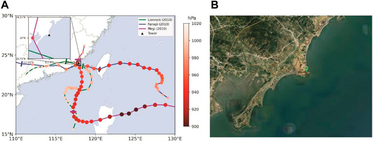
FIGURE 1. (A) Tracks of Lionrock (green curve), Fanapi (blue curve), and Megi (purple curve). Dots show the storm center positions every 6 h, with the minimum central pressure indicated with colors. The time analyzed is the time encompassed between the two short crosses on each track. The site of the observational tower is indicated by the black triangle. An enlarged view of the tower position is also present in the upper-left corne. (B) The ground environment surrounding the tower, with the light green sector symbol marking the tower location.

Wind Data From the Tower Observations

The data used in this study are obtained from a multi-level weather tower placed in Chihu Town, Zhangpu, Fujian Province, China, at the 24.036°N latitude and 117.897°E longitude (Figure 1A). The minimal distance of the tower from the coastline is about 150 m (Figure 2B), and it lies 29 m above sea level. The surface around the tower is mainly rubble soil with scattered shrubs. WindMaster Pro 3D supersonic anemometers manufactured by British Gill are fitted at 27-, 43-, 60-, and 82-m heights. Correspondingly, the tower’s four observational heights are 56, 72, 89, and 111 m above sea level. The sampling frequency for the three-dimensional wind speed is 20 Hz. Quality control for the three-dimensional wind fields is conducted using a spectral analysis method following Zhang et al. (2009) and Ming and Zhang (2018). This data has been utilized to examine the near-surface turbulent cascade features (Tang et al., 2015) and vertical eddy diffusivity and mixing length in the TC boundary layer (Tang et al., 2018).

FIGURE 2

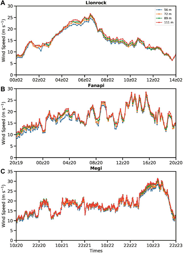
FIGURE 2. Time series of the 10-min averages of wind velocity observed with the tower in Typhoon (A) Lionrock from 11 to 14 UTC 2 September, (B) Fanapi from 20 UTC 19 to 20 UTC 20 September, and (C) Megi from 10 UTC 20 to 22 UTC 23 October 2010. The blue, orange, green, and red curves represent the averaged wind speed at z = 56, 72, 89, and 111 m, respectively.

In this study, we put the spotlight on the wind observations of Lionrock from 1600 UTC 1 September to 0600 on 2 September, Fanapi from 1200 UTC 19 September to 1200 UTC 20 September, and Megi from 0200 UTC 20 October to 1400 UTC 23 October 2010 (Figure 1A). These periods are chosen when the horizontal wind velocities averaged in 10 min are above 10 m s⁻¹ at the four observational heights. Figure 2A shows that the 10-min averaged wind velocities of Typhoon Lionrock gradually increased as the system approached the tower, peaking around 0630 UTC 2 September 2010 and followed by a gradual decrease in speed. Similar wind speed evolution was observed in Typhoon Fanapi, with the maximum averaged wind speed occurring when the TC center neared the tower around 1500 UTC 20 September 2010 (Figure 2B). The maximum wind speed observed by the tower was greater than 30 m s⁻¹ in Typhoon Megi near 1100 UTC 23 October 2010 (Figure 2C), and it rapidly weakened afterward due to the proximity of the eye.

An IBL can appear in an area of horizontal advection across a discontinuity in varying surface properties (Deaves, 1981; Garratt, 1990). In particular, the IBL should continue to deepen until its depth has adjusted to the underlying surface, dependent on the surface roughness (Savelyev and Taylor, 2015). IBL development was frequently observed at landfalls of TCs, particularly in the land-water transition (Powell, 1982; Knupp et al., 2006; Hirth et al., 2012). Regardless of mesoscale effects, neutral static stability is widely considered to dominate the TC boundary layer (Kepert, 2012), and the velocity IBL height ($h_{VIBL}$) can be estimated as

$h_{VIBL}=c{Z}_R{\left(\frac{X}{Z_R}\right)}^{0.8},(1)$

where $Z_R$ denotes the roughness length, $c$ is a stability constant generally valued at 0.28 for a statistically neutral environment (Simiu and Scanlan, 1996; Wood, 1982), and $X$ indicates the downstream distance. As indicated in Fang et al. (2018), a $Z_R$ value of 0.05 m is selected for the surface featured by rubble soil with scattered shrubs, and a maximum land fetch is about 400 m for onshore winds. Thus, a $h_{VIBL}$ value approximates to be 18.56 m at this land fetch. Moreover, prior studies have revealed that the stress IBL height ($h_{SIBL}$) approximately doubles $h_{VIBL}$ (Rao et al., 1974; Garratt, 1990). Correspondingly, $h_{SIBL}$ is ∼37.1 m near the tower (Fang et al., 2018), implying that the surface likely has a striking effect on the local stress above the first observational height but below the second height of the tower. Therefore, given the stress IBL, we limit our focus to the DH properties from the second to the fourth levels that lie in a constant flux layer.

Figures 3A–C show the wind speed spectra of three-dimensional wind speeds at z = 72 m for one good flux run in Typhoon Fanapi, which is displayed in the log-log plots of frequency. The spectrum patterns conform to the -5/3 slope of Kolmogorov (1941) power law. Correspondingly, the cospectra and cumulative summations of cospectra of the flux run are shown in Figures 2D,E, respectively. A good flux run approaches a constant value in both high and low frequencies, which represents stationarity. Such a scenario can be confirmed by the flatness near the high- and low-frequency tails from 0.001 to 10 Hz in Figure 2E. Lastly, 106, 116, and 111 good flux runs are validated at the 72-, 89-, and 111-m observational heights, respectively, for the three TCs.

FIGURE 3

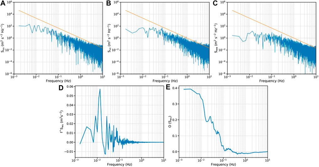
FIGURE 3. (A–C) Plots of the power spectra for the three-dimensional wind velocities at z = 72 m from a good flux run of Typhoon Fanapi. The orange lines represent the -5/3 slope. Plots of the (D) cospectra and (E) cumulative summations of cospectra of along-wind momentum flux from this good flux run.

Estimation Methods for Dissipative Heating

As noted in the introduction, two methods have usually been used to estimate DH values associated with TCs. One is proposed by Bister and Emanuel (1998), hereafter referred to as the BE method. In the BE method, DH is estimated by calculating the momentum flux and drag coefficient. According to the eddy correlation method, the momentum flux ($\widehat{\tau }$) is defined as:

$\widehat{\tau }=\rho \left(-\overline{w^{\prime }{u}^{\prime }}\widehat{i}-\overline{w^{\prime }{v}^{\prime }}\widehat{j}\right),(2)$

where $u^{\text{'}}$, $v^{\text{'}}$, and $w^{\text{'}}$ represent the turbulent fluctuations of longitudinal, lateral, and vertical components of wind speed, and the overbar represents 10-min averaging. $\rho$ is the air density. The momentum flux magnitude in the surface layer can be calculated as follows:

$\tau =\rho u^{\ast 2}=\rho C_d{U}^2,(3)$

where $u^{\ast }$ represents the friction velocity, $U$ is the average horizontal wind speed at the given height, and $C_d$ is the drag coefficient. Therefore, the friction velocity can be defined as

$u^{\text{*}}={\left(\frac{\left|\widehat{\tau }\right|}{\rho }\right)}^{1/2}.(4)$

Additionally, shear production is assumed to balance dissipation as heat in a weak wind environment (Businger and Businger, 2001). Based on the Monin-Obukhov similarity theory (Monin and Obukhov, 1954), shear production can be estimated using $u^{\ast }$. The dissipation term ($\epsilon$) can, therefore, be computed by

$\epsilon =\frac{u^{\ast 3}}{\kappa z},(5)$

where $\kappa$ is the Von Kármán constant and equals 0.4.

In the absence of an IBL, DH can be calculated by vertically integrating the dissipation rate and can be expressed by

$DH=\rho \overline{\epsilon }{Z}_1=\rho \frac{u^{\ast 3}}{\kappa }\ln \left(\frac{Z_1}{Z_R}\right),(6)$

where $Z_1$ is the observational height and the overbar represents the average value.

However, given the stress IBL in the tower site, it is difficult to directly apply Eq. 6 to calculate DH at the observational levels because when the $u^{\ast }$ values within the IBL exceed approximately 0.4 m s⁻¹ they are much larger than those above the IBL (Fang et al., 2018). Therefore, the $\epsilon$ magnitudes estimated by Eq. 5 are significantly larger at z = 56 m than at the upper levels (Figures 4A,B). Nevertheless, we can estimate the integrated DH between two levels (for example, at $Z_1$ and $Z_2$) above the stress IBL but in the surface layer as follows:

$\rho \frac{u^{\ast 3}}{\kappa }\ln \left(\frac{Z_2}{Z_1}\right)=\rho u^{\ast 2}U\left(Z_2\right)-\rho u^{\ast 2}U\left(Z_1\right),(7)$

if $\epsilon$ decreases linearly with height. Here, based on the Monin-Obukhov similarity theory, the difference in wind speed ($U$) between the two layers is

$U\left(Z_2\right)-U\left(Z_1\right)=\frac{u^{\ast }}{\kappa }\ln \left(\frac{Z_2}{Z_1}\right).(8)$

FIGURE 4

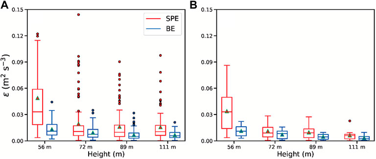
FIGURE 4. Boxplots of the dissipative rates at the four observational levels using (A) all the good runs and (B) good runs coexisting at all the levels at a given time [with the lower and upper quartiles as the lower and upper limits of the box, respectively; the median (line in the box); the mean (triangles), and outliers (black circles)]. Blue and red colors indicate the BE and turbulent spectra methods, respectively.

Figure 4B shows that the mean $\epsilon$ value regarding the sets of concurrent good runs at all the heights indeed decreases with height approximately in a linear manner. Thus, Eq. 7 may be applied herein to assess the integrated DH within the constant flux layer.

The other method for the DH estimation is to directly estimate the dissipation rate of turbulence by spectral analysis and vertically integrating the dissipation rate. According to Zhang (2010) and Ming and Zhang (2018), $\epsilon$ can be estimated from the spectral density of the longitudinal velocity whose spectra show a $f^{-5/3}$ power law, and given by

$\epsilon ={\alpha }_u^{-3/2}\frac{2\pi f}{U}{\left[f{S}_{uu}\left(f\right)\right]}^{3/2},(9)$

where ${\alpha }_u$ is the one-dimensional Kolmogorov constant, being generally equal to 0.5 (Sreenivasan, 1995), $S_{uu}$ is the power spectral density of horizontal wind speed, and $f$ is the frequency. Note that using the direct method involves satisfying an assumption that $\epsilon$ is constant with height. Figures 4A,B show the $\epsilon$ properties calculated by Eq. 9 for all the good run samples and the simultaneous samples at the four observations levels, respectively. The $\epsilon$ values are statistically significantly larger at the first observational level (z = 56 m) than at upper levels (Figures 4A,B). Additionally, there are no significant differences in the $\epsilon$ magnitude between the three levels above (at the 95% confidence level based on the permutation test). This result further suggests that the first observational level resides likely within the IBL. Therefore, based on the turbulent spectra method, the integrated DH between two levels above the stress IBL but within the surface layer can be given by

$\rho \underset{Z_1}{\overset{Z_2}{{\displaystyle \int }}}\epsilon dz=\rho \overline{\epsilon }\left(Z_2-Z_1\right),(10)$

with $\epsilon$ being estimated by Eq. 9. Furthermore, Figure 4 also shows that the mean $\epsilon$ values calculated by the theoretical method are less than those directly estimated by the turbulent spectra method at each level.

As noted in previous studies, there are apparent differences in the BE and turbulent spectra methods for estimating the DH value. The former assumes that frictionally dissipated kinetic energy is wholly converted to heat, while the latter directly measures DH considering the turbulent flow characteristics.

Results

As introduced above, the DH estimation with the BE method first involves the computation of friction velocity and the drag coefficient. Figure 5A portrays the friction velocities measured from the tower observations versus mean wind speed. We can see that the bin-averaged friction velocities tend to linearly increase with wind speed when the wind speed is lower than 25 m s⁻¹, whereas those at z = 54, 89, and 111 m level off at wind speeds of 25 m s⁻¹ (Figure 5A). This result is slightly smaller than that in Zhao et al. (2015), which indicated that the wind speed threshold for friction velocity level-off was between 26 and 30 m s⁻¹.

FIGURE 5

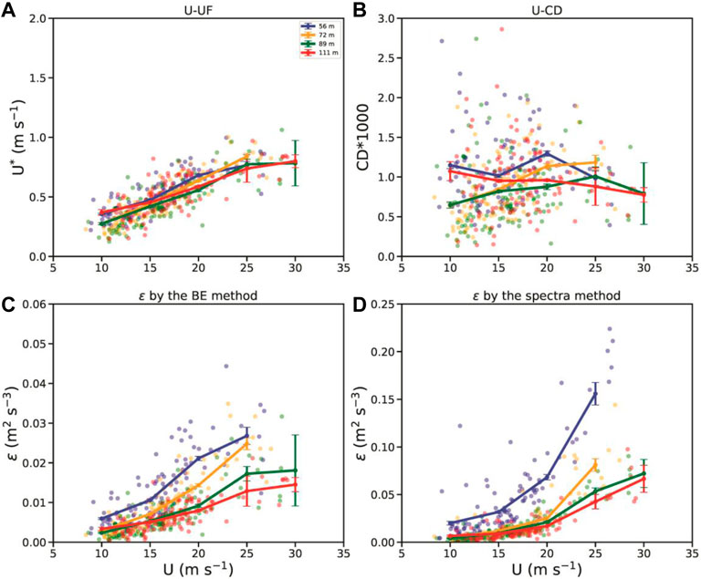
FIGURE 5. Plots of (A) the friction velocity, (B) drag coefficients, and (C) dissipative rates estimated with the BE method and (D) turbulent spectra method as a function of the mean wind speed. The blue, orange, green, and red solid lines with error bars indicate the bin-averaged values of the two variables at z = 56, 72, 89, and 111 m, respectively. The error bars represent the 95% confidence interval.

Figure 5B shows the drag coefficient as a function of wind speed at different levels. Not surprisingly, at the lowest level (z = 56 m), the drag coefficient values are the largest when the wind velocity is smaller than 25 m s⁻¹. The averaged drag coefficient values range between 0.001 and 0.0015, close to prior results over shallow water (Zhao et al., 2015; Ming and Zhang, 2018). Previous studies indicated that the magnitude of the drag coefficient tended to increase with increasing wind speed when the speed was lower than the critical value (Powell et al., 2003; Jarosz et al., 2007; Holthuijsen et al., 2012). However, such a tendency is not captured at z = 56 m, likely because of the limited samples at lower wind speed (Figure 5B). The drag coefficient values go down as the altitude rises (e.g., z = 72 and 89 m). At these two levels, the drag coefficients increase with increasing wind speed. In particular, the estimated drag coefficient value at z = 89 m turns to lower when the wind speed exceeds 25 m s⁻¹, indicative of saturation of the drag coefficient.

Figure 5C depicts the dissipative rates estimated by Eq. 5 as a function of the mean wind speed. The dissipative rates estimated by the theoretical method tend to increase with increasing wind speed as the wind velocity is smaller than 25 m s⁻¹, consistent with the finding in Zhang (2010). According to Eq. 5, the dissipative rate is predicted to be a smaller magnitude at a higher level. This pattern can be reflected by the bin-averaged values in Figure 5C, except at z = 89 and 111 m with the wind velocity around 10 m s⁻¹. In contrast, the dissipative rates directly estimated by the turbulent spectra method are indicated in Figure 5D. At the levels above the stress IBL, the differences in the mean dissipative rates are minimal when the wind speed is less than 20 m s⁻¹, and they subtly increase when the wind speed exceeds 20 m s⁻¹. Nevertheless, the variation of the dissipative rates with height seems smaller than implied in the BE approach. In addition, a comparison of Figures 5C,D further suggests that the mean dissipative rates estimated by shear production are smaller at relatively high wind speeds than those estimated by the turbulent spectra method, which is also revealed in Figure 4 and previous findings over ocean conditions (Zhang, 2010). It is worth noting that the mean directly-measured dissipative rates at z = 56 m are 2–3 times those at the upper levels (Figure 5D), indicating that the stress within IBL indeed greatly reinforces the local dissipation.

The DH integrated between two levels above the stress IBL, calculated by the two methods mentioned above as a function of mean wind speed, is depicted in Figure 6. Note that the samples with good runs simultaneously identified at both levels are analyzed. The integrated DH values tend to increase with increasing wind velocities. However, when the wind speed is less than 15 m s⁻¹, the integrated DH increases much slower with increasing wind speed. The integrated DH estimated by the BE method tends to be constant when the wind speed is less than 15 m s⁻¹ (Figures 6A–C). When the wind speed is more than 15 m s⁻¹, the integrated DH values significantly increase. Notably, the integrated DH estimated by the turbulent spectra method increases much more rapidly with increasing wind speed than those estimated by the BE method. As a result, the integrated DH values produced by the two methods gradually bifurcate each other when the wind velocity is larger than 20 m s⁻¹, particularly between z = 72 and 111 m (Figure 6C).

FIGURE 6

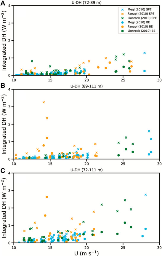
FIGURE 6. Plots of the DH integrated between (A) 72 and 89 m, (B) 89 and 111 m, and (C) 72 and 111 m by the BE method (diagonal-cross symbols) and turbulent spectra method (solid dots) as a function of the mean wind speed. The green, orange, and blue colors indicate the results regarding Lionrock, Fanapi, and Megi, respectively. Note that the samples with good runs simultaneously identified at both levels are used.

Figure 7 further compares the integrated DH values estimated with the BE method versus the turbulent spectra method for the good flux runs. In detail, most integrated DH values estimated with the turbulent spectra method are larger than those estimated with the BE method (Figures 7A–C), with the integrated DH estimated with the BE method approximating 1/4–1/3 of the DH estimated with the turbulent spectra method within the constant flux layer.

FIGURE 7

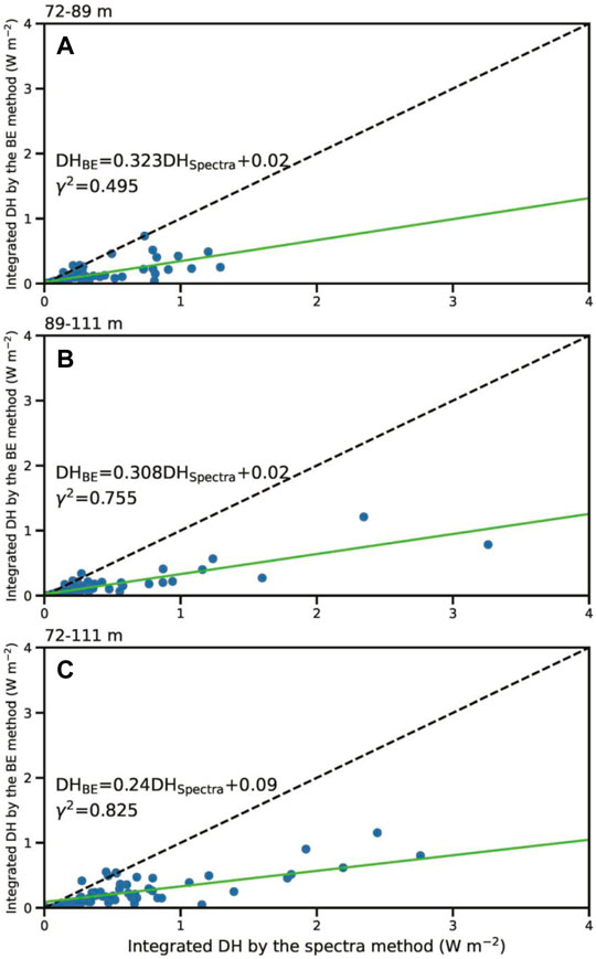
FIGURE 7. Comparisons between the DH integrated between (A) 72 and 89 m, (B) 89 and 111 m, and (C) 72 and 111 m by the BE method and the turbulent spectra method. The black dashed lines represent the 1:1 ratio, and the solid green lines represent the least-squares best fit. The relationship equations and coefficients of determination are also shown. Note that the samples with good runs simultaneously identified at both levels are used.

The integrated DH properties above the IBL are further quantified with the bin-averaged values in Table 1. As noted above, the integrated DH estimated with the BE method is much smaller than that estimated with the turbulent spectra method above the stress IBL. The integrated DH values estimated with both methods increase with increasing wind speed, and not surprisingly, they also increase with layer depth for each wind speed bin. Table 1 indicates that the integrated DH calculated with the turbulent spectra method grows much more rapidly with increasing wind speed than that calculated with the theoretical method. For instance, the mean DH values integrated between z = 89 and 111 m with the turbulent spectra method (BE method) rise dramatically from 0.39 (0.15) to 1.02 (0.40) W m⁻² for the wind speed bin increasing from 20 to 25 m s⁻¹.

TABLE 1

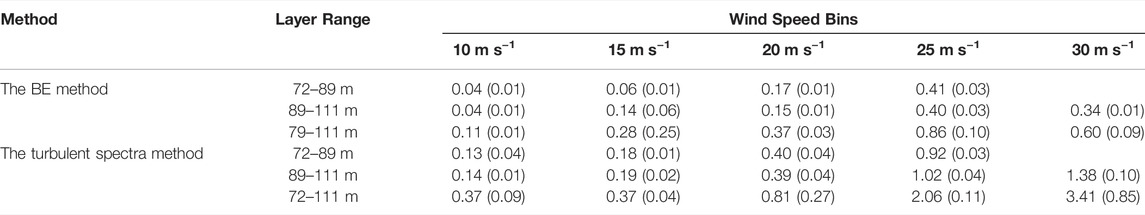
TABLE 1. The bin-averaged integrated DH values (W m⁻²) estimated with the turbulent spectra method and the BE method, with the standard deviations included in parentheses.

As pointed out in previous studies, the BE method that assumes all the work done by friction converted into DH within the TC boundary layer overestimates DH magnitude (Zhang, 2010; Zhang et al., 2011; Ming and Zhang, 2018). As a result, during TC landfalls, the IBL DH estimated using the BE formula is much larger (even larger than an order of magnitude) than that estimated using the turbulent spectra method (Zhang et al., 2011). In the current study, DH properties within the stress IBL cannot be estimated due to the limited observations within the IBL. Nevertheless, the multi-level observations from the coastal tower furnish an opportunity to document the DH properties integrated between levels above the stress IBL. Unlike the DH within the IBL, the integrated DH based on the turbulent spectra method is significantly larger than that estimated based on the BE method.

Summary

In this paper, wind observations collected from a multi-level observation tower near the coast are used to estimate the DH properties above the IBL during the landfalls of three typhoons. The main interest is quantifying the vertically integrated DH in landfalling TC conditions. In addition, the integrated DH estimations based on the BE method and turbulent spectra method are also made for comparison.

The results demonstrate that, above the stress IBL, the integrated DH values estimated with the BE method and the turbulent spectra method increase with increasing wind speed. Additionally, the integrated DH calculated with the turbulent spectra method rises more rapidly with increasing wind speed than that estimated with the BE method. However, the integrated DH calculated with the BE method is much smaller than that calculated with the turbulent spectra method, although DH overestimation based on the BE method has been widely recognized. The larger integrated DH with the turbulent spectra method than the BE method is mainly related to greater dissipative rates estimated using the former above the IBL.

An implication of the tower-based observational study results here is assessing the numerically modeled DH and surface layer height in landfalling TC circulation, which may contribute to improvements in surface layer schemes in numerical modeling of TCs. However, one of the limitations of the present study is that the wind speed observed here is under severe tropical storm force. In a region close to the water, how the complex surface state can modulate the vertical variation of DH above the IBL requires further dedicated investigation.

Data Availability Statement

The raw data supporting the conclusions of this article will be made available by the authors, without undue reservation.

Author Contributions

KZ: Investigation and Writing—review. QL: Writing—review and editing. JT: Investigation.

Funding

This work was jointly supported by the National Key Research and Development Program of China under grant 2017YFC1501601 and the National Natural Science Foundation of China under grants 42175005, 41875054, 41730961, 41730960, and 41775065. The observational data in this study were from a field experiment supported by the Experiment of Typhoon Intensity Changes in the Coastal Area (EXOTICCA).

Conflict of Interest

The authors declare that the research was conducted in the absence of any commercial or financial relationships that could be construed as a potential conflict of interest.

The reviewer JL declared a shared affiliation with the authors KZ, QL to the handling editor at the time of review.

Publisher’s Note

All claims expressed in this article are solely those of the authors and do not necessarily represent those of their affiliated organizations, or those of the publisher, the editors and the reviewers. Any product that may be evaluated in this article, or claim that may be made by its manufacturer, is not guaranteed or endorsed by the publisher.

Acknowledgments

We thank the reviewers for their valuable comments, which improved the paper.

References

Bister, M., and Emanuel, K. A. (1998). Dissipative Heating and Hurricane Intensity. Meteorl. Atmos. Phys. 65, 233–240. doi:10.1007/bf01030791

CrossRef Full Text | Google Scholar

Businger, S., and Businger, J. A. (2001). Viscous Dissipation of Turbulence Kinetic Energy in Storms. J. Atmos. Sci. 58, 3793–3796. doi:10.1175/1520-0469(2001)058<3793:vdotke>2.0.co;2

CrossRef Full Text | Google Scholar

Cheng, X., Fei, J., Huang, X., and Zheng, J. (2012). Effects of Sea spray Evaporation and Dissipative Heating on Intensity and Structure of Tropical Cyclone. Adv. Atmos. Sci. 29, 810–822. doi:10.1007/s00376-012-1082-3

CrossRef Full Text | Google Scholar

Deaves, D. M. (1981). Computations of Wind Flow Over Changes in Surface Roughness. J. Wind Eng. Ind. Aerodyn. 7, 65–94. doi:10.1016/0167-6105(81)90068-4

CrossRef Full Text | Google Scholar

Edwards, J. M. (2019). Sensible Heat Fluxes in the Nearly Neutral Boundary Layer: The Impact of Frictional Heating within the Surface Layer. J. Atmos. Sci. 76, 1039–1053. doi:10.1175/jas-d-18-0158.1

CrossRef Full Text | Google Scholar

Emanuel, K. A. (1986). An Air-Sea Interaction Theory for Tropical Cyclones. Part I: Steady-State Maintenance. J. Atmos. Sci. 43, 585–605. doi:10.1175/1520-0469(1986)043<0585:aasitf>2.0.co;2

CrossRef Full Text | Google Scholar

Fang, P., Zhao, B., Zeng, Z., Yu, H., Lei, X., and Tan, J. (2018). Effects of Wind Direction on Variations in Friction Velocity with Wind Speed under Conditions of strong Onshore Wind. J. Geophys. Res. 123, 7340–7353. doi:10.1029/2017jd028010

CrossRef Full Text | Google Scholar

Garratt, J. R. (1992). The Atmospheric Boundary Layer. UK: Cambridge University Press, 316.

Google Scholar

Garratt, J. R. (1990). The Internal Boundary Layer—A Review. Boundary-Layer Meteorol. 50, 171–203. doi:10.1007/bf00120524

CrossRef Full Text | Google Scholar

Hirth, B. D., Schroeder, J. L., Weiss, C. C., Smith, D. A., and Biggerstaff, M. I. (2012). Research Radar Analyses of the Internal Boundary Layer over Cape Canaveral, Florida, during the Landfall of Hurricane Frances (2004). Wea. Forecast. 27, 1349–1372. doi:10.1175/waf-d-12-00014.1

CrossRef Full Text | Google Scholar

Holthuijsen, L. H., Powell, M. D., and Pietrzak, J. D. (2012). Wind and Waves in Extreme Hurricanes. J. Geophys. Res. 117, C09003. doi:10.1029/2012jc007983

CrossRef Full Text | Google Scholar

Jarosz, E., Mitchell, D. A., Wang, D. W., and Teague, W. J. (2007). Bottom-up Determination of Air-Sea Momentum Exchange under a Major Tropical Cyclone. Science 315, 1707–1709. doi:10.1126/science.1136466

PubMed Abstract | CrossRef Full Text | Google Scholar

Jin, Y., Thompson, W. T., Wang, S., and Liou, C.-S. (2007). A Numerical Study of the Effect of Dissipative Heating on Tropical Cyclone Intensity. Wea. Forecast. 22, 950–966. doi:10.1175/waf1028.1

CrossRef Full Text | Google Scholar

Kepert, J. D. (2012). Choosing a Boundary Layer Parameterization for Tropical Cyclone Modeling. Mon. Wea. Rev. 140, 1427–1445. doi:10.1175/mwr-d-11-00217.1

CrossRef Full Text | Google Scholar

Kieu, C. (2015). Revisiting Dissipative Heating in Tropical Cyclone Maximum Potential Intensity. Q.J.R. Meteorol. Soc. 141, 2497–2504. doi:10.1002/qj.2534

CrossRef Full Text | Google Scholar

Knupp, K. R., Walters, J., and Biggerstaff, M. (2006). Doppler Radar and Profiler Observations of Boundary Layer Variability during the Landfall of Tropical Storm Gabrielle. J. Atmos. Sci. 63, 234–251. doi:10.1175/jas3608.1

CrossRef Full Text | Google Scholar

Kolmogorov, A. N. (1941). The Local Structure of Turbulence in Incompressible Viscous Fluid for Very Large Reynolds Number. Dokl. Akad. Nauk SSSR. 30, 301–303.

Google Scholar

Ming, J., and Zhang, J. A. (2018). Direct Measurements of Momentum Flux and Dissipative Heating in the Surface Layer of Tropical Cyclones during Landfalls. J. Geophys. Res. Atmos. 123, 4926–4938. doi:10.1029/2017jd028076

CrossRef Full Text | Google Scholar

Monin, A. S., and Obukhov, A. M. (1954). Basic Laws of Turbulent Mixing in the Ground Layer of the Atmosphere. Akad. Nauk. SSSR Geofiz. Inst. 151, 163–187.

Google Scholar

Powell, M. D. (1982). The Transition of the Hurricane Frederic Boundary-Layer Wind Field from the Open Gulf of Mexico to Landfall. Mon. Wea. Rev. 110, 1912–1932. doi:10.1175/1520-0493(1982)110<1912:ttothf>2.0.co;2

CrossRef Full Text | Google Scholar

Powell, M. D., Vickery, P. J., and Reinhold, T. A. (2003). Reduced Drag Coefficient for High Wind Speeds in Tropical Cyclones. Nature 422, 279–283. doi:10.1038/nature01481

PubMed Abstract | CrossRef Full Text | Google Scholar

Rao, K. S., Wyngaard, J. C., and Coté, O. R. (1974). The Structure of the Two-Dimensional Internal Boundary Layer over a Sudden Change of Surface Roughness. J. Atmos. Sci. 31, 738–746. doi:10.1175/1520-0469(1974)031<0738:tsottd>2.0.co;2

CrossRef Full Text | Google Scholar

Savelyev, S. A., and Taylor, P. A. (2005). Internal Boundary Layers: I. Height Formulae for Neutral and Diabatic Flows. Boundary-Layer Meteorol. 115, 1–25. doi:10.1007/s10546-004-2122-z

CrossRef Full Text | Google Scholar

Simiu, E., and Scanlan, R. H. (1996). Wind Effects on Structures: Fundamentals and Applications to Design. New York: John Wiley & Sons, 589.

Google Scholar

Sreenivasan, K. R. (1995). On the Universality of the Kolmogorov Constant. Phys. Fluids 7, 2778–2784. doi:10.1063/1.868656

CrossRef Full Text | Google Scholar

Tang, J., Byrne, D., Zhang, J. A., Wang, Y., Lei, X.-t., Wu, D., et al. (2015). Horizontal Transition of Turbulent cascade in the Near-Surface Layer of Tropical Cyclones. J. Atmos. Sci. 72, 4915–4925. doi:10.1175/jas-d-14-0373.1

CrossRef Full Text | Google Scholar

Tang, J., Zhang, J. A., Aberson, S. D., Marks, F. D., and Lei, X. (2018). Multilevel Tower Observations of Vertical Eddy Diffusivity and Mixing Length in the Tropical Cyclone Boundary Layer during Landfalls. J. Atmos. Sci. 75, 3159–3168. doi:10.1175/jas-d-17-0353.1

CrossRef Full Text | Google Scholar

Wood, D. H. (1982). Internal Boundary Layer Growth Following a Step Change in Surface Roughness. Boundary-Layer Meteorol. 22, 241–244. doi:10.1007/bf00118257

CrossRef Full Text | Google Scholar

Ying, M., Zhang, W., Yu, H., Lu, X., Feng, J., Fan, Y., et al. (2014). An Overview of the China Meteorological Administration Tropical Cyclone Database. J. Atmos. Ocean. Technol. 31, 287–301. doi:10.1175/jtech-d-12-00119.1

CrossRef Full Text | Google Scholar

Zhang, D.-L., and Altshuler, E. (1999). The Effects of Dissipative Heating on hurricane Intensity. Mon. Wea. Rev. 127, 3032–3038. doi:10.1175/1520-0493(1999)127<3032:teodho>2.0.co;2

CrossRef Full Text | Google Scholar

Zhang, J. A., Drennan, W. M., Black, P. G., and French, J. R. (2009). Turbulence Structure of the Hurricane Boundary Layer between the Outer Rainbands. J. Atmos. Sci. 66, 2455–2467. doi:10.1175/2009jas2954.1

CrossRef Full Text | Google Scholar

Zhang, J. A. (2010). Estimation of Dissipative Heating Using Low-Level In Situ Aircraft Observations in the hurricane Boundary Layer. J. Atmos. Sci. 67, 1853–1862. doi:10.1175/2010jas3397.1

CrossRef Full Text | Google Scholar

Zhang, J. A., Marks, F. D., Montgomery, M. T., and Lorsolo, S. (2011). An Estimation of Turbulent Characteristics in the Low-Level Region of Intense Hurricanes Allen (1980) and Hugo (1989). Mon. Wea. Rev. 139 (5), 1447–1462. doi:10.1175/2010mwr3435.1

CrossRef Full Text | Google Scholar

Zhao, Z.-K., Liu, C.-X., Li, Q., Dai, G.-F., Song, Q.-T., and Lv, W.-H. (2015). Typhoon Air-Sea Drag Coefficient in Coastal Regions. J. Geophys. Res. Oceans 120, 716–727. doi:10.1002/2014jc010283

CrossRef Full Text | Google Scholar