DriftScalarDyFoam: An OpenFOAM-Based Multistage Solver for Drifting Snow and Its Distribution Around Buildings

1 Introduction

Aeolian transport, which is typified by snow drifting, manifests as the interaction between wind and a large number of tiny snow particles. In cold regions, a related phenomenon may cause various types of problems such as equipment failure, traffic interruption, and structural collapse (Tominaga, 2018). Much research for snow drifting has been carried out through field measurements (Mellor and Fellers, 1986; Pomeroy and Gray, 1990; Ma et al., 2021), wind tunnel tests (Lü et al., 2012; Zhou et al., 2016b), and numerical simulations (Tominaga et al., 2011a; Huang et al., 2011; Zhou et al., 2016a).

For snowdrift related to buildings, the Steady-RANS CFD simulation based on the Eulerian approach was proven to provide sufficiently accurate results with a low computational cost (Uematsu et al., 1991; Tominaga et al., 2011b; Tominaga et al., 2011a; Zhou et al., 2016a; Zhu et al., 2017; Wang et al., 2019; Zhou et al., 2020), which ensures that relevant disaster prediction can be carried out in the shortest possible time. However, snow drifting will generally last hours or even days; during this, meteorological conditions and snow distribution may have significant changes. Therefore, Tominaga et al. (2011a) developed a system for predicting snow distribution combining a mesoscale meteorological model and a CFD model, in which weather conditions are updated in each time step. Zhou et al. (2016a) developed this method to predict the snow distribution on a roof, in which a multistage numerical model is proposed to consider the feedback of the snow distribution to the airflow. Related methods have been expanded in Zhu et al. (2017) and Wang et al. (2019): the former aims to introduce the RBF-based dynamic mesh method into the roof snow distribution, and the latter uses the immersion boundary method to obtain a more robust simulation process.

However, the previous research studies are more inclined to use commercial CFD software (e.g., Ansys Fluent), which is unfavorable for researchers who want to reproduce or improve this method. OpenFOAM (or Open-source Field Operation And Manipulation) (Weller et al., 1998) is an open-source suite of libraries and applications designed to solve computational fluid dynamics (CFD) problems, by which we modularize the airflow, snow transport, and the evolution of snow distribution (dynamic mesh), and the solver developed by these modules is named driftScalarDyFoam. Powered by native OpenFOAM tools, driftScalarDyFoam supports complex three-dimensional geometries, automated time step processing/snow evolution, and rich programmable interface, which will have a positive impact on the improvement of related methods and industrial production for snow engineering.

2 Methods

2.1 Snow Transport

The continuity and Navier–Stokes equations, used as governing equations for incompressible airflow, are expressed as follows:

$\frac{\partial u_i}{\partial x_i}=0(1)$

and

$\frac{\partial u_i}{\partial t}+u_j\frac{\partial u_i}{\partial x_j}=-\frac{1}{{\rho }_a}\frac{\partial p}{\partial x_i}+\frac{\partial }{\partial x_j}\left[\left(\nu +{\nu }_{\text{t}}\right)\left(\frac{\partial u_i}{\partial x_j}+\frac{\partial u_j}{\partial x_i}\right)\right],(2)$

where u_i is the airflow velocity, subscript i (i = 1, 2, 3) denotes the streamwise, spanwise, and vertical directions; p is the pressure; ν is viscosity; and ν_t is turbulent viscosity (or eddy viscosity).

The snow transport in a suspension layer is calculated by using a convection–diffusion equation (Tominaga et al., 2011a; Zhou et al., 2016a; Zhu et al., 2017; Kang et al., 2018), in which the snow phase is considered to have the same velocity as the airflow in the horizontal direction, and a virtual velocity in the direction of gravity is added to the convection term to represent the falling of snow. The complete equation is expressed as

$\frac{\partial \varphi }{\partial t}+\frac{\partial \varphi u_j}{\partial x_j}+\frac{\partial \varphi w_f}{\partial x_3}=\frac{\partial }{\partial x_j}{D}_t\frac{\partial \varphi }{\partial x_j},(3)$

where the diffusion of snow in turbulence is considered to be consistent with the eddy diffusion, the coefficient of which can be expressed as

$D_t=\frac{{\nu }_t}{S{c}_t},(4)$

where ϕ is the drift density of snow; w_f is the falling velocity of snow; ν_t is the turbulent viscosity; and Sc_t is the turbulent Schmidt number, which describes the ratio between the rates of turbulent transport of momentum and the turbulent transport of mass.

Snow particle saltation can be divided into four subprocesses including the aerodynamic entrainment, particle trajectories, particle-bed collisions, and wind modification (Huang et al., 2011), and for this kind of complicated transportation process, it is difficult to use the Eulerian approach to express at the macro-level. Thus, a formula (Eq. 5) in which the constant was determined by observation in the drifting boundary layer proposed by Pomeroy and Gray (1990) is widely used in related research studies for snow drifting (Naaim et al., 1998; Kang et al., 2018).

$Q_{\text{sal}}=\frac{0.68{\rho }_a{u}_{\ast t}}{g{u}_{\ast }}\left(u_{\ast }^2-u_{\ast t}^2\right),(5)$

where ρ_a is the air density; u_∗ is the local friction velocity; u_∗ is the threshold friction velocity; and g is the gravitational acceleration.

However, Tominaga et al. (2011b) point out that the snow drifting around a building is in non-equilibrium due to acceleration and deceleration, which means that Eq. 5 is more suitable for snow drifting in flat terrains rather than that around buildings. Thus, a new approach to evaluating the transport rate in the saltation layer is proposed by Tominaga et al. (2011b), which is expected to be more efficient than fixing the saltation flux in non-equilibrium regions, and the details of this approach are included in the erosion and deposition model (Section 2.2).

2.2 Erosion and Deposition

The establishment of the erosion and deposition model can reflect the evolution of snow distribution during snow drifting, which was first proposed by Uematsu et al. (1991). The total mass exchange rate M_total can be expressed as

$M_{\text{total}}=M_{\text{dep}}+M_{\text{ero}}.(6)$

Here, M_dep is the deposition rate, which is affected by the falling velocity and drift density of snow near the surface where u_* < u_*t:

$M_{\text{dep}}=-{\varphi }_p{w}_f\left(1-\frac{u_{*}^2}{u_{*t}^2}\right)A_{\text{hol}}(7)$

and M_ero is the erosion rate which occurs where u_∗ > u_∗t:

$M_{\text{ero}}=-A_{\text{ero}}{u}_{\ast }^2\left(1-\frac{u_{\ast t}^2}{u_{\ast }^2}\right)A_{\text{hol}},(8)$

where A_hol is the horizontal area of the computational grid; A_ero is a coefficient that represents the bonding strength of snowpack, and A value of A_ero = 7 × 10^–4 is employed according to a previous study (Zhou et al., 2016a).

When erosion occurs, Fick’s laws of diffusion (Fick, 1855) are adopted on the snow surface, which relates the diffusive flux to the gradient of the drift density and can be expressed as a Neumann condition:

${\left.\left(\frac{\partial \varphi }{\partial \mathbf{n}}\right)\right|}_{\text{surface}}=-\frac{1}{D_t}\frac{\left|M_{\text{ero\hspace{0.17em}}}\right|}{A_{\text{hol}}},(9)$

where n is the unit normal vector of the boundary face.

3 Numerical Implementation

DriftScalarDyFoam is an incompressible separate solver considering the pseudo-transient assumption of long-period snow drifting and the dynamic evolution of snowdrift, implemented within the OpenFOAM framework, and parallelized with MPI. Its source code is available and released under the GNU General Public License (GPL).

3.1 Pseudo-Transient Continuation

The redistribution of the snow surface can be described as a first-order time-dependent ordinary differential equation (ODE) for snow mass exchange M:

$\frac{dM}{dt}=-f\left(\varphi ,\mathbf{u}\right),(10)$

where the drift density ϕ and the wind velocity u determine the erosion and deposition of snow and affect the snow distribution, and the snow distribution in turn affects the wind velocity and drift density.

An explicit Euler method is adopted to discretize the continuous time, which is expressed as

$M_{n+1}=M_n+\delta f_n\left(\varphi ,\mathbf{u}\right),(11)$

where the wind velocity and drift density in old time steps will be used to calculate the snow distribution of new time steps. However, it should be pointed out that the explicit scheme is often limited by the step size and is conditionally stable. Therefore, using a single time step to predict the snow distribution may be inaccurate.

Since Zhou et al. (2016a) pointed out that the snow drifting is in a practical quasi-steady state in long-period snowstorms, the pseudo-transient continuation is introduced in this study, which is a method for finding the steady-state solution of time-evolving partial differential equations by making an initial guess and then evolving the solution forward using a time-stepper. Therefore, “stage,” a sub-concept of “time step,” is introduced in our model. We define a large time step as a stage and find a steady-state solution in it, and then update the snow distribution of the next time step with the previous calculation result. This actually simplifies the evolution of snow drifting in a specific time step as a linear process. The specific procedures are as follows and are shown in Figure 1:

Step 1) Prepare a computational domain and initialize fields.

Step 2) Enter a new global time step and start the sub-cycle in this global time step.

Step3) Update all fields with the SIMPLE algorithm as a steady-state scalar transport with one-way coupling, in which the equations of pressure p and velocity u are solved first, and the drift density ϕ is solved later. The boundary condition based on erosion/deposition according to Eq. 9 will be updated in each sub-cycle iteration.

Step4) Calculate the mass exchange rate M_total based on the friction velocity near the snow surface and the drift density at the center of the cell adjacent to the snow surface (Eqs 6–8).

Step5)Adjust the snow surface according to the mass exchange rate M_total and the time step of each stage. If the current global time step is not the final time step, update the physical time and go back to Step 2.

FIGURE 1

FIGURE 1. Flowchart of the pseudo-transient scheme for long-period evolution of snow drifting.

3.2 Dynamic Evolution of Snow Distribution

In Section 3.1, it is mentioned that the mesh will be adjusted according to the current mass exchange M on the snow surface in each global time step. In previous research studies, Zhou et al. (2016a) generated the approximate smooth curves through a series of separated nodes from old coordinates and their high increments based on erosion/deposition. Zhu et al. (2017) implemented the interpolation from face data to node data based on the radial basis function (RBF) on the snow surface and then adjusted the internal cell with the logarithmic law along the z-direction.

In this study, a more practical method is applied, in which the inverse distance between the boundary point and its neighbor face center is used as the weight to help implement the interpolation from face value to node value. This method is similar to the RBF interpolation method, but the inverse proportional function we used does not meet the Gaussian distribution. After the interpolation, we specify a vector field C to mark the cell displacement and generate the displacement C|_surface of the snow surface as the Dirichlet boundary condition:

$\mathbf{C}{|}_{\text{surface}}=\frac{M_{\text{total}}}{{\rho }_s{A}_{\text{hol}}},(12)$

where ρ_s is the bulk density of snow. Then, a Laplacian equation is solved to smooth the displacement of internal cells:

$D\frac{{\partial }^2{C}_i}{\partial x_j^2}=0,(13)$

where D is the diffusivity. In most scenarios, we hope that the cells near the dynamic surface can maintain similar displacement, and those cells far from this region have a smaller displacement. Thus, the value of the diffusivity is related to the quadratic inverse distance from internal cell centers to the snow surface. We discretize and solve Eq. 13 with the finite volume method for unstructured grids, just like the solution of the airflow velocity u. The boundary conditions of C_i is easily obtained—the grid size is static at locations far from the snow surface, where C_i = 0, and the C_i value on the snow surface is related to the mass exchange rate M_total caused by erosion/deposition (Eq. 12).

4 Validation

4.1 Case I: Snow Distribution on a Flat Roof

The snow distribution on a flat roof is a typical research case for snow drifting around buildings (Zhou et al., 2016a; Zhou et al., 2016b; Liu et al., 2019). This case is designed to study the snow distribution on the roof after long-period snow drifting, and the snow load obtained is meaningful for structural design.

The calculation model used in this study is the prototype described by Liu et al. (2019), whose size is 3H × 2H × H, and an 80-cm-high snow cover is stacked on the roof in the initial state (see Tables 1, 2 for more details). The neutral equilibrium atmospheric boundary layer profile proposed by Yang et al. (2009) is used to determine the incoming airflow and whether the wind direction is along the positive direction of x-axis:

$u\left(z\right)=\frac{u_{\ast }}{\kappa }\ln \left(\frac{z-d+z_0}{z_0}\right)(14)$

$k=\frac{{\left(u^{\ast }\right)}^2}{\sqrt{C_{\mu }}}\sqrt{C_1\ln \left(\frac{z-d+z_0}{z_0}\right)+C_2}(15)$

$\epsilon =\frac{{\left(u^{\ast }\right)}^3}{\kappa \left(z-d+z_0\right)}\sqrt{C_1\ln \left(\frac{z-d+z_0}{z_0}\right)+C_2},(16)$

where d is ground–normal displacement height; z₀ is aerodynamic roughness height; the von Karman constant κ is 0.40; and C₁ = 0, C₂ = 1, and C_μ = 0.09, which means that we actually used the turbulence boundary conditions suggested by Richards and Hoxey (1993).

TABLE 1

TABLE 1. Overview of parameters used in simulation of snow drifting in case I.

TABLE 2

TABLE 2. Computation conditions used in simulation of snow drifting in case I.

Zhou et al. (2016b) point out that there is a significant difference in snow distribution on the flat roof in the initial and final states, in which the number of stages is set to 3 according to the 2.5D wind tunnel test. However, there is no study to point out the appropriate stage of the snow drifting on a 3D flat roof. Figure 2A depicts the variation of the total snow mass on the flat roof using different number of stages. On the one hand, with the evolution of physical time, snow mass on the roof tends to stabilize. On the other hand, using more stages helps the solution become more smooth and converge at approximately 3.4 × 104 kg. More details can be found in Figures 2B–H. Results using 5 or 10 stages present discontinuities in front of the roof (x/H < 1.0), and due to excess snow transport, there is a significant accumulation in the rear of the separation point (0.5 < x/H < 1.5). As the number of stages increases (25 or 50 stages), these two phenomena decreases, but the erosion prediction in the front region is still excessive. Finally, there is no significant difference when using more number of stages (100 or 250 stages).

FIGURE 2

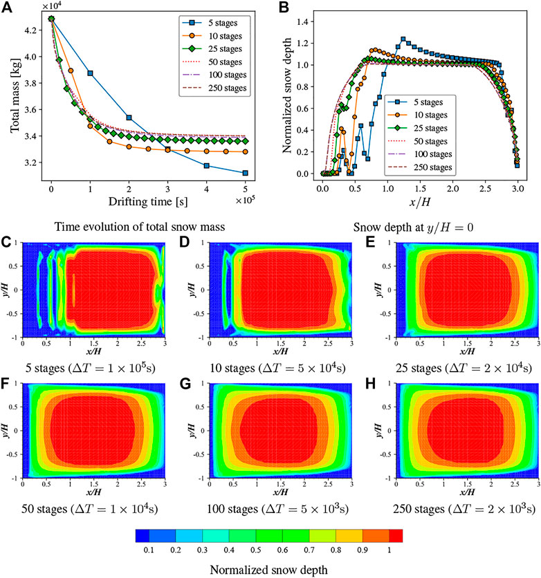
FIGURE 2. Snow distribution on the roof using different numbers of calculation stages. (E,F) depict the final snow distribution (T = 5 × 10⁵ s) using different number of stages. (A) Time evolution of total snow mass. (B) Snow depth at y/H = 0. (C) 5 stages (ΔT = 1 × 10⁵ s). (D) 10 stages (ΔT = 5 × 10⁴ s). (E) 25 stages (ΔT = 2 × 10⁴ s). (F) 50 stages (ΔT = 1 × 10⁴ s). (G) 100 stages (ΔT = 5 × 10³ s). (H) 250 stages (ΔT = 2 × 10³ s).

An interesting phenomenon is that the time required for erosion to reach a stable time in the front region is much shorter than that that in the rear region (Figures 3, 5A), which is caused by the large friction velocity in the front region in earlier stages (Figure 4A). When stage 10 is reached, the maximum friction velocity in the front region (excluding the exposed roof) is limited to the threshold friction velocity (0.2 m/s), and the snow distribution here is thus stabilized. In contrast, the evolution of snow distribution in the rear region is gradual. The friction velocity in the outer side gradually decreases, and the inner friction velocity gradually increases, and both of them finally stabilize near the threshold friction velocity (0.2 m/s) (Figure 4B). This phenomenon indicates that there is a strong interaction between the erosion and airflow in the rear region.

FIGURE 3

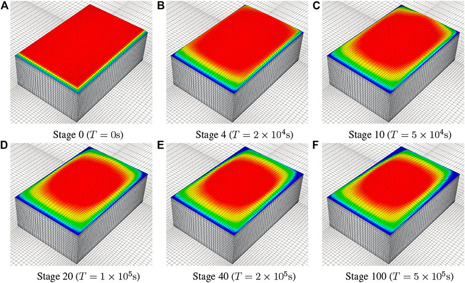
FIGURE 3. Time evolution of the snow distribution on a 3D flat roof using 100 stages (ΔT = 5 × 10³ s). (A) Stage 0 (T = 0 s). (B) Stage 4 (T = 2 × 10⁴ s). (C) Stage 10 (T = 5 × 10⁴ s). (D) Stage 20 (T = 1 × 10⁵ s). (E) Stage 40 (T = 2 × 10⁵ s). (F) Stage 100 (T = 5 × 10⁵ s).

FIGURE 4

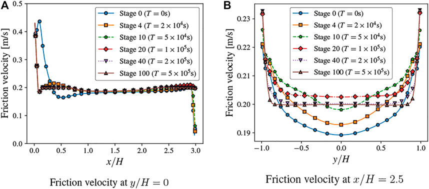
FIGURE 4. Variation of friction velocity using a total of 100 stages (ΔT = 5 × 10³ s). (A) Friction velocity at y/H = 0. (B) Friction velocity at x/H = 2.5.

The comparison with the wind tunnel test indicates that our simulation results are within the expected range (Figure 5B), especially in the front region. U(H) used in this study (4.84 m/s) corresponds to 5.81 m/s in the wind tunnel test of Liu et al. (2019), so the distribution in the rear region (x/H > 2) is also in a reasonable range. However, we have pointed out that there is a strong correlation between the snow erosion and airflow characteristics in the rear region. Therefore, the snow distribution here is more sensitive to atmospheric boundary conditions and the roughness height of the snow surface. More parameter analyses will be carried out in subsequent research.

FIGURE 5

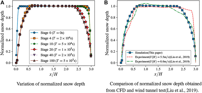
FIGURE 5. Snow depth at y/H = 0 using a total of 100 stages (ΔT = 5 × 10³ s). (A) Variation of normalized snow depth. (B) Comparison of normalized snow depth obtained from CFD and wind tunnel test (Liu et al., 2019).

4.2 Case II: Snow Distribution Around Single Cube

In regions of high snowfall and strong wind in winter, snowdrift is formed around buildings due to long-period snow drifting, which may cause difficulties for vehicular traffic and pedestrians (Tominaga et al., 2011a). Therefore, snow distribution around a single cube is simulated according to the observation of (Oikawa et al., 1999), which can help the urban planning in the cold region.

The model and simulation parameters of Case II are similar to Case I (Table 3, 4). According to the conditions of observation (Oikawa et al., 1999), the size of the building is set to 1 m × 1 m × 1 m. At the end of the calculation, we normalized the snow distribution according to the snow depth far from the building.

TABLE 3

TABLE 3. Overview of parameters used in simulation of snow drifting in case II.

TABLE 4

TABLE 4. Computation conditions used in simulation of snow drifting in case II.

Figure 6 depicts the snow distribution around the building. The separation flow on both sides of the building causes large area erosion, and the inner corner vortex leads to deposition, which is similar to the simulation results of Tominaga et al. (2011a) (Figure 7B). However, Figure 7B depicts that the simulation has excessive prediction on both deposition and erosion. It should be pointed out that one-way coupling used in our model leads to an excessive prediction of airflow velocity near the snow surface, and turbulent flow causes the variable falling velocity of snow particle, which leads to the aforementioned limitations.

FIGURE 6

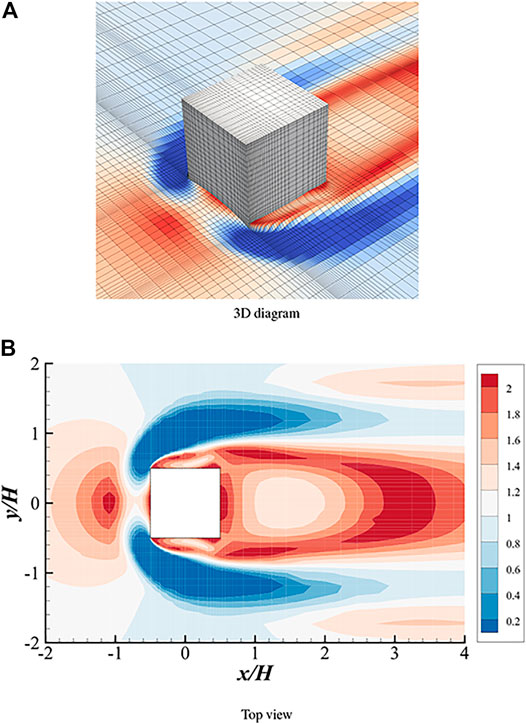
FIGURE 6. Snow distribution around the cube at T = 1 × 10⁴ s. The color bar represents the normalized snow depth, and the reference snow depth is the snow depth at the outlet, which is in the absence of building. (A) 3D diagram. (B) Top view.

FIGURE 7

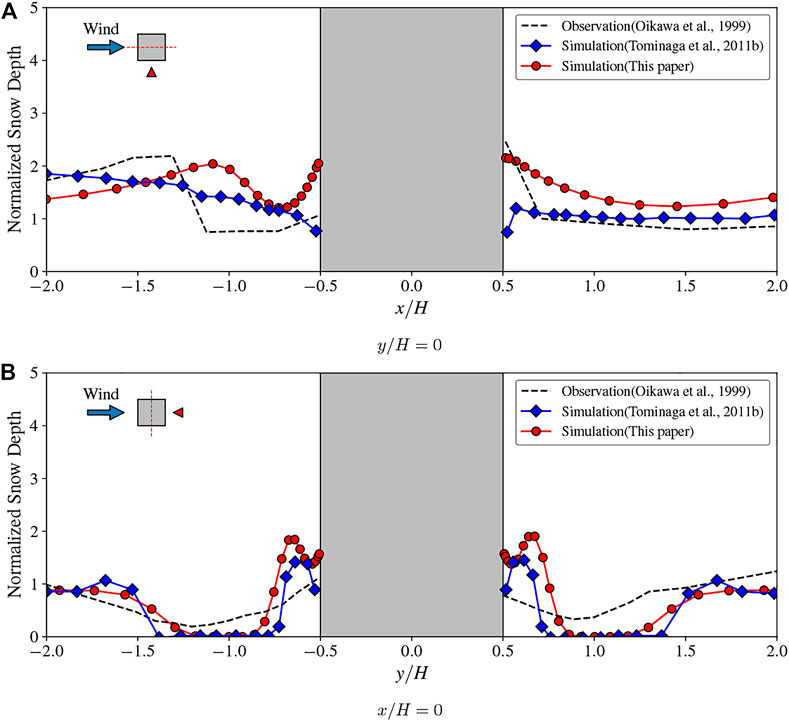
FIGURE 7. Comparison of normalized snow depths obtained from previous CFD simulation (Tominaga et al., 2011a) and field measurements (Oikawa et al., 1999). (A) y/H = 0. (B) x/H = 0.

In the comparison of snow depth at y/H = 0, we find that although similar methods are used, our solver seems to get a more accurate result in the deposition prediction in the front and rear regions of the building than that in Tominaga et al. (2011a). This may be derived from our different erosion/deposition formulas (Eqs 7, 8). According to Figure 8, the incoming flow forms reverse flow on the windward side due to the obstruction of the building, resulting in less snow deposition at this location. A similar trend also exists on the leeward side, but the vortex formed on the leeward side is larger, so the snow distribution is more flat. This shows that the erosion/deposition model we use is more sensitive to the airflow.

FIGURE 8

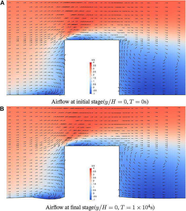
FIGURE 8. Velocity vectors and contours around the cube. (A) Airflow at initial stage (y/H = 0, T = 0 s). (B) Airflow at final stage (y/H = 0, T = 1 × 10⁴ s).

5 Conclusion

This study mainly introduces the solver driftScalarDyFoam developed based on OpenFOAM, which refers to the classic snow transport model and erosion/deposition formula, and incorporates the multistage model to achieve simulations with long-term duration or complex meteorological conditions.

Through the prediction of snow distribution on flat roofs and around buildings, driftScalarDyFoam has been shown to be robust and reliable in its results, which depicts its versatility in the research and production of snow engineering. Compared with previous numerical studies (Tominaga et al., 2011b; Zhou et al., 2016a), our simulations also obtained similar results to observation data, and based on the scalability and parameterization of driftScalarDyFoam, we carried out a discussion on the number of stages during the snow drifting transport process. The “stage” concept of driftScalarDyFoam enables this solver to adapt to time-varying meteorological data and snow distribution, which is beneficial for industrial applications.

However, the limitation of the theoretical model hinders the accuracy of this solver, including the one-way coupling between snow and airflow and turbulence effect on snow particles. In addition, the application of this model in mountainous regions (Gerber et al., 2017; Li et al., 2018) still needs further verification. Further development on this existing framework with more advanced and efficient physical models is necessary.

Data Availability Statement

The original contributions presented in the study are included in the article/Supplementary Material; further inquiries can be directed to the corresponding author.

Author Contributions

XC: conceptualization of this study, methodology, software, validation, formal analysis, data curation, writing—original draft, and visualization. ZY: project administration and funding acquisition.

Funding

This project is jointly supported by the National Natural Science Foundation of China (Nos. 51378428 and 52178506).

Conflict of Interest

The authors declare that the research was conducted in the absence of any commercial or financial relationships that could be construed as a potential conflict of interest.

Publisher’s Note

All claims expressed in this article are solely those of the authors and do not necessarily represent those of their affiliated organizations, or those of the publisher, the editors, and the reviewers. Any product that may be evaluated in this article, or claim that may be made by its manufacturer, is not guaranteed or endorsed by the publisher.

Supplementary Material

The Supplementary Material for this article can be found online at: https://www.frontiersin.org/articles/10.3389/feart.2022.822140/full#supplementary-material

References

Fick, A. (1855). Ueber Diffusion. Ann. Phys. Chem. 170, 59–86. doi:10.1002/andp.18551700105._eprint

CrossRef Full Text | Google Scholar

Gerber, F., Lehning, M., Hoch, S. W., and Mott, R. (2017). A Close-ridge Small-Scale Atmospheric Flow Field and its Influence on Snow Accumulation. J. Geophys. Res. Atmos. 122, 7737–7754. doi:10.1002/2016JD026258

CrossRef Full Text | Google Scholar

Huang, N., Sang, J., and Han, K. (2011). A Numerical Simulation of the Effects of Snow Particle Shapes on Blowing Snow Development. J. Geophys. Res. 116, a–n. doi:10.1029/2011JD016657

CrossRef Full Text | Google Scholar

Kang, L., Zhou, X., van Hooff, T., Blocken, B., and Gu, M. (2018). CFD Simulation of Snow Transport over Flat, Uniformly Rough, Open Terrain: Impact of Physical and Computational Parameters. J. Wind Eng. Ind. Aerodynamics 177, 213–226. doi:10.1016/j.jweia.2018.04.014

CrossRef Full Text | Google Scholar

Li, G., Wang, Z. S., and Huang, N. (2018). A Snow Distribution Model Based on Snowfall and Snow Drifting Simulations in Mountain Area. J. Geophys. Res. Atmos. doi:10.1029/2018JD028434

CrossRef Full Text | Google Scholar

Liu, Z., Yu, Z., Zhu, F., Chen, X., and Zhou, Y. (2019). An Investigation of Snow Drifting on Flat Roofs: Wind Tunnel Tests and Numerical Simulations. Cold Regions Sci. Tech. 162, 74–87. doi:10.1016/j.coldregions.2019.03.016

CrossRef Full Text | Google Scholar

Lü, X., Huang, N., and Tong, D. (2012). Wind Tunnel Experiments on Natural Snow Drift. Sci. China Technol. Sci. 55, 927–938. doi:10.1007/s11431-011-4731-3

CrossRef Full Text | Google Scholar

Ma, W., Li, F., and Zhou, X. (2021). An Empirical Model of Snowdrift Based on Field Measurements: Profiles of the Snow Particle Size and Mass Flux. Cold Regions Sci. Tech. 189, 103312. doi:10.1016/j.coldregions.2021.103312

CrossRef Full Text | Google Scholar

Mellor, M., and Fellers, G. (1986). Concentration and Flux of Wind-Blown Snow, 86. US Army Corps of Engineers, Cold Regions Research & Engineering Laboratory.

Google Scholar

Naaim, M., Naaim-Bouvet, F., and Martinez, H. (1998). Numerical Simulation of Drifting Snow: Erosion and Deposition Models, A. Glaciology., 26. Publisher: Cambridge University Press, 191–196. doi:10.3189/1998AoG26-1-191-196doi:10.1017/s0260305500014798

CrossRef Full Text | Google Scholar

Oikawa, S., Tomabechi, T., and Ishihara, T. (1999). One-day Observations of Snowdrifts Around a Model Cube. J. Snow Eng. Jpn. 15, 283–291. doi:10.4106/jsse.15.4_283

CrossRef Full Text | Google Scholar

Pomeroy, J. W., and Gray, D. M. (1990). Saltation of Snow. Water Resour. Res. 26, 1583–1594. doi:10.1029/WR026i007p01583._eprint

CrossRef Full Text | Google Scholar

Richards, P. J., and Hoxey, R. P. (1993). Appropriate Boundary Conditions for Computational Wind Engineering Models Using the K-ϵ Turbulence Model. J. Wind Eng. Ind. Aerodynamics 46-47, 145–153. doi:10.1016/0167-6105(93)90124-7

CrossRef Full Text | Google Scholar

Tominaga, Y. (2018). Computational Fluid Dynamics Simulation of Snowdrift Around Buildings: Past Achievements and Future Perspectives. Cold Regions Sci. Tech. 150, 2–14. doi:10.1016/j.coldregions.2017.05.004

CrossRef Full Text | Google Scholar

Tominaga, Y., Mochida, A., Okaze, T., Sato, T., Nemoto, M., and Motoyoshi, H. (2011a). Development of a System for Predicting Snow Distribution in Built-Up Environments: Combining a Mesoscale Meteorological Model and a CFD Model. J. Wind Eng. Ind. Aerodynamics 99, 460–468. doi:10.1016/j.jweia.2010.12.004

CrossRef Full Text | Google Scholar

Tominaga, Y., Okaze, T., and Mochida, A. (2011b). CFD Modeling of Snowdrift Around a Building: An Overview of Models and Evaluation of a New Approach. Building Environ. 46, 899–910. doi:10.1016/j.buildenv.2010.10.020

CrossRef Full Text | Google Scholar

Uematsu, T., Nakata, T., Takeuchi, K., Arisawa, Y., and Kaneda, Y. (1991). Three-dimensional Numerical Simulation of Snowdrift. Cold Regions Sci. Tech. 20, 65–73. doi:10.1016/0165-232X(91)90057-N

CrossRef Full Text | Google Scholar

Wang, J., Liu, H., Xu, D., Chen, Z., and Ma, K. (2019). Modeling Snowdrift on Roofs Using Immersed Boundary Method and Wind Tunnel Test. Building Environ. 160, 106208. doi:10.1016/j.buildenv.2019.106208

CrossRef Full Text | Google Scholar

Weller, H. G., Tabor, G., Jasak, H., and Fureby, C. (1998). A Tensorial Approach to Computational Continuum Mechanics Using Object-Oriented Techniques. Comput. Phys., 12. American Institute of Physics, 620–631. doi:10.1063/1.168744.Publisher

CrossRef Full Text | Google Scholar

Yang, Y., Gu, M., Chen, S., and Jin, X. (2009). New Inflow Boundary Conditions for Modelling the Neutral Equilibrium Atmospheric Boundary Layer in Computational Wind Engineering. J. Wind Eng. Ind. Aerodynamics 97, 88–95. doi:10.1016/j.jweia.2008.12.001

CrossRef Full Text | Google Scholar

Zhou, X., Kang, L., Gu, M., Qiu, L., and Hu, J. (2016a). Numerical Simulation and Wind Tunnel Test for Redistribution of Snow on a Flat Roof. J. Wind Eng. Ind. Aerodynamics 153, 92–105. doi:10.1016/j.jweia.2016.03.008

CrossRef Full Text | Google Scholar

Zhou, X., Qiang, S., Peng, Y., and Gu, M. (2016b). Wind Tunnel Test on Responses of a Lightweight Roof Structure under Joint Action of Wind and Snow Loads. Cold Regions Sci. Tech. 132, 19–32. doi:10.1016/j.coldregions.2016.09.011

CrossRef Full Text | Google Scholar

Zhou, X., Zhang, Y., Kang, L., and Gu, M. (2020). RANS CFD Simulations Can Be Successfully Used for Simulating Snowdrift on Roofs in a Long Period of Snowstorm. Building Simulation 13, 1157–1163. doi:10.1007/s12273-020-0651-0

CrossRef Full Text | Google Scholar

Zhu, F., Yu, Z., Zhao, L., Xue, M., and Zhao, S. (2017). Adaptive-mesh Method Using RBF Interpolation: A Time-Marching Analysis of Steady Snow Drifting on Stepped Flat Roofs. J. Wind Eng. Ind. Aerodynamics 171, 1–11. doi:10.1016/j.jweia.2017.09.008

CrossRef Full Text | Google Scholar