Swarm-TEC Satellite Measurements as a Potential Earthquake Precursor Together With Other Swarm and CSES Data: The Case of Mw7.6 2019 Papua New Guinea Seismic Event

On May 14, 2019, a strong M_w = 7.6 shallow earthquake occurred in Papua New Guinea. This paper explores for the first time the analysis of total electron content (TEC) products measured for 6 months by GPS antenna onboard Swarm satellites, to detect possible seismo-ionospheric anomalies around the time and location of the above-mentioned earthquake. The night-time vertical total electron content (VTEC) time series measured using Swarm satellites Alpha and Charlie, inside the earthquake Dobrovolsky’s area show striking anomalies 31 and 35 days before the event. We successfully verified the possible presence of concomitant anomalous values of in situ electron density detected by the new Chinese satellite dedicated to search for electromagnetic earthquake precursors [China Seismo-Electromagnetic Satellite (CSES)-01]. On the other hand, the analysis of VTEC night time measured by Swarm Bravo shows gradual and abnormal increase of the VTEC parameter from about 23 days before the earthquake, which descends 3 days before the earthquake and reaches its lowest level around the earthquake day. We also analyzed the time series and tracks of other six in situ parameters measured by Swarm satellites, electron density from CSES, and also GPS-TEC measurements. As it is expected from the theory, the electron density anomalous variations acknowledge the Swarm VTEC anomalies, confirming that those anomalies are real and not an artifact of the analysis. The comparative analysis with measurements of other Swarm and CSES sensors emphasizes striking anomalies about 2.5 weeks before the event, with a clear pattern of the whole anomalies typical of a critical system as the earthquake process is for Earth. A confutation analysis outside the Dobrovolsky area and without significant seismicity shows no anomalies. Therefore based on our study, the VTEC products of Swarm satellites could be an appropriate precursor aside from the other measured plasma and magnetic parameters using Alpha, Bravo, and Charlie Swarm and CSES satellites that can be simultaneously analyzed to reduce the overall uncertainty.

Introduction

Since the seismological community generally emphasizes the great difficulty of earthquake prediction by analyzing seismic data (e.g., Matsumura, 2009), or even the impossibility of such an enterprise (e.g., Geller, 1997), many researchers have dedicated their efforts to search for alternative non-seismic precursors. Up to now, many papers and reports have been released to emphasize the importance of this kind of earthquake precursors. It seems that the results of ionospheric precursors have been more reliable than lithospheric and atmospheric ones (Parrot, 1995; Hayakawa and Molchanov, 2002; Pulinets and Boyarchuk, 2004; Freund, 2009; Pulinets and Ouzounov, 2011; Sorokin and Pokhotelov, 2014; Guo et al., 2015; Piscini et al., 2017; Liu, 2018; Cianchini et al., 2020; Ouzounov et al., 2021). The seismo-ionospheric anomalies might be observed in the D, E, and F layers around the time and location of the event. Therefore, remote sensing satellite sensors could be good tools to gather and monitor ionospheric precursors above seismic-prone areas (Akhoondzadeh et al., 2010; De Santis et al., 2015).

Swarm mission (launched on 22 November, 2013) is a constellation of three identical satellites, Alpha (A), Bravo (B), and Charlie (C), placed in quasi-polar orbits at an altitude between 440 (Alpha and Charlie) and 510 km (Bravo) (Friis-Christensen et al., 2006). These satellites include magnetic and plasma sensors: 1) an absolute scalar magnetometer (ASM), which measures the strength of the magnetic field and provides scalar measurements of the magnetic field to calibrate the vector field magnetometer; 2) a vector field magnetometer (VFM), which makes high-precision measurements of the intensity and direction of the magnetic field; and 3) the EFI instrument, which is composed of the Langmuir probe and thermal ion imager. The Langmuir probe provides plasma data such as electron density, Ne, electron temperature, Te, and spacecraft electric potential, V (Haagmans et al., 2013).

To date, some papers have investigated plasma and magnetic field parameters around the time and location of some strong earthquakes using Swarm satellites’ data (De Santis et al., 2017; Akhoondzadeh et al., 2018; Marchetti and Akhoondzadeh, 2018; Akhoondzadeh et al., 2019; Marchetti et al., 2019a; Marchetti et al., 2019b). A very recent paper has established the statistical significance of the anomalies of these parameters observed by Swarm satellites as anticipating strong earthquakes all over the world for the last 5 years of data (De Santis et al., 2019).

However, there has not yet been any scientific report indicating the Swarm vertical total electron content (VTEC) data analysis as possibly associated with powerful earthquakes.

The Global Navigation Satellite System (GNSS) transmits signals, while the ground receivers and the one mounted on the Swarm satellites receive them. By the analysis of transmission delays, it is possible to infer the total amount of electrons in the ionospheric path crossed by the signals. Therefore slant total electron content (STEC), which is defined as the integrated electron density along the line of sight from the ground or Swarm receivers to GNSS satellites, is estimated by analyzing the mentioned delay (Swarm Level 2 Processing System, 2019). This means that Swarm-TEC data contain information about the integrated electron density from about 400 km above Swarm satellites (Swarm Expert Support Laboratories, 2017), so analogous to what happened with the CHAMP satellite (Noja et al., 2013).

Relative STEC can be estimated by the following equation:

$\mathit{STEC}=\frac{f_1^2\times f_2^2}{f_1^2-f_2^2}\times \frac{L_1-L_2}{K}(1)$

where f₁ and f₂ are carrier frequencies of GNSS signals, L₁ and L₂ are ambiguity-corrected carrier phase observations, and $K\approx 40.3 m^3{s}^{-2}$ is a conversion factor. By considering the elevation angle of the GNSS satellite as seen from ground or Swarm GPS receivers (and also altitude of the Swarm satellite in this case), VTEC is calculated from STEC (Foelsche and Kirchengast, 2002; Yizengaw et al., 2006; Noja et al., 2013) only for allowable elevation angles (Swarm Level 2 Processing System, 2019). When the Swarm satellites are close to the edge of Dobrovolsky area, to VTEC, satellite data also contribute to the electron density data from a little outside the Dobrovolsky area. However, we think that this effect is very little and can be neglected with respect to most data that are inside the Dobrovolsky area.

This paper presents for the first time the results of Swarm-TEC data analysis for a specific large earthquake. In detail, we analyzed the Swarm data during the period of January 01 to June 30, 2019 inside the Dobrovolsky’s area (Dobrovolsky et al., 1979; see also Swarm-TEC Data) of the Papua New Guinea earthquake. The mentioned earthquake had a magnitude M_w = 7.6 and took place at 12:58:25 UTC (LT = UTC+λ_epicenter/15 = 23:08:48) on May 14, 2019, 46 km SSE of Namatanai in Papua New Guinea (4.051°S, 152.597°E) at an estimated shallow depth of about 10 km (Figure 1). The region where the event occurred is critical from a tectonical point of view: the Australian plate moves in East–North East direction with respect to the Pacific plate, and many microplates are involved in the plate boundary. In particular, the main event of May 14, 2019 occurred in the boundary between South Bismark and Manus microplates. The estimated rupture of the fault was about $50\times 10 k{m}^2$, with a peak slip of about 25 m (Chen et al., 2019). In the past, in the same location, other several big earthquakes already occurred (for example, M8.0 on November 16, 2000 localized at 3.980S 152.169E, 33 km depth).

FIGURE 1

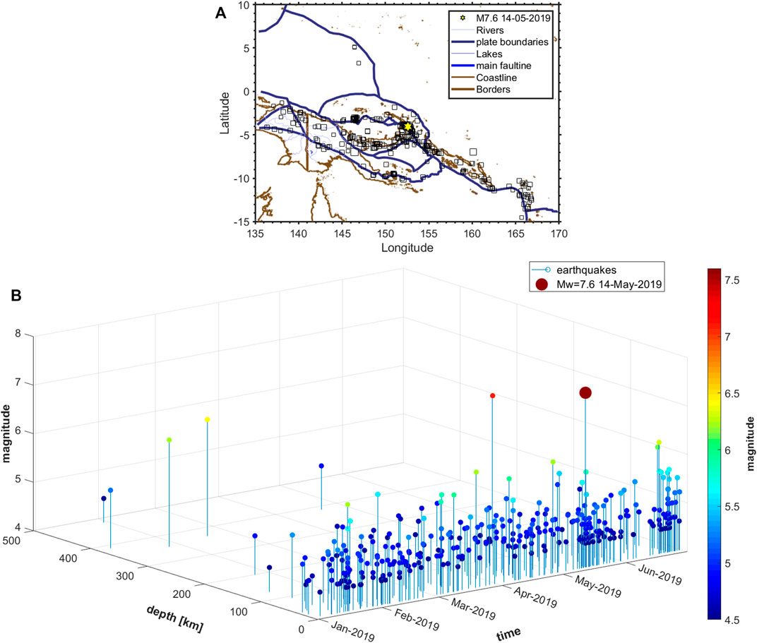
FIGURE 1. Representation of the M4.5+ earthquakes that occurred inside the Dobrovolsky area of the Mw = 7.6 May 14, 2019 Papua New Guinea earthquake from January 01 to June 30, 2019 retrieved from USGS catalogue (https://earthquake.usgs.gov/earthquakes). (A) Geographical map of the seismic events with the geographical features and main faults. The epicenter is depicted by a yellow star. (B) Graph of the temporal, depth, and magnitude of the selected M4.5+ events. The main shock has been evidenced by the largest circle.

Figure 1 shows that the seismic events with a magnitude greater than or equal to 4.5 occurred in the area investigated in this period from January 01 to June 30, 2019 (USGS catalogue; https://earthquake.usgs.gov/earthquakes). We underline a particular strong event of Mw = 7.1 that occurred on May 06, 2019 at 21:19:37 UTC localized at 6.975°S 146.449°E at a depth of about 146 km. Despite the relative great depth of this event, it is not possible to exclude any coseismic effect in the ionosphere when the results are discussed.

Observations

Solar and Geomagnetic Data

To exclude the solar geomagnetic disturbances in the analysis of potential seismo-ionospheric precursors, the a_p and D_st magnetic indices and the solar radio flux (i.e., F10.7) are checked, defining quiet solar geomagnetic conditions such as a_p < 25 nT, |Dst| ≤ 20 nT, and F10.7 < 120 SFU. Figure 2 illustrates the variations of a_p, D_st and F10.7 indices, and solar wind and IMF intensity during the period of January 01 to June 30, 2019. A star symbol shows the earthquake time. The x-axis indicates the day relative to the earthquake day. The y-axis represents the universal time in a) and b), the F10.7 (SFU) value in c), and the values of solar wind speed (in km/s) and IMF intensity (in nT) in d). In addition, to monitor the space weather conditions for what concerns the Interplanetary Magnetic Field (IMF), we retrieved the data by the solar satellite observatory Advanced Composition Explorer (ACE), placed in the Sun–Earth L1 Lagrangian point (at 1.4 million kilometers from Earth), have been investigated. In particular, in Figure 2D), the intensity of IMF from the magnetometer and the alpha-particle solar wind speed from the solar wind ion composition spectrometer instrument are represented. Thus, the eventual anomalies in the ionosphere detected during high solar wind speed and IMF are excluded by the analysis because they are more likely the effects of an ionosphere–magnetosphere coupling rather than lithosphere–atmosphere–ionosphere coupling. The identification of high solar activity has been evaluated by characterizing two investigated physical observables (a vector of the interplanetary magnetic field defined by the components IMF_X, IMF_Y, IMF_Z, and its intensity IMF_F and the intensity of alpha-particle solar wind) by median and interquartile over the analyzed 6-month data, and defining a high activity when one of the investigated solar quantities (i.e., IMF_X, IMF_Y, IMF_Z, IMF_F, and alpha-particle solar wind) overpasses the median by 1.5 times the interquartile range, which corresponds to the thresholds of 7.59 nT for IMF_F (scalar intensity of IMF) and 524 km/s for solar wind speed. These conditions have been applied, taking into account two ways of possible magnetosphere–ionosphere coupling: one is the impact of solar wind onto the ionosphere, and the other is the electromagnetic field coupling. For the former, the time of flight of the particles from ACE satellite to Swarm or CSES has been estimated for the specific time while for the latter, it requires about 5 s so it can be considered instantaneous for this work. Consequently, our basic hypothesis is that the detected remaining anomalous variations of ionospheric parameters in quiet solar geomagnetic conditions might be associated with seismic activities.

FIGURE 2

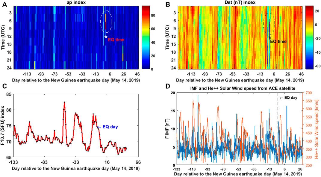
FIGURE 2. (A–D) show the variations of a_p, D_st, and solar radio flux (F10.7) indices and two parameters (magnetic field scalar intensity and He²⁺ solar wind speed) of the IMF recorded from ACE satellite, respectively, during the period of January 01 to June 30, 2019.

High geomagnetic activity is clearly seen on the earthquake date, when the a_p index reaches the unusual values of 67 nT and 94 nT between 04:00 and 09:00 UTC. The unusual variations of the a_p index are also seen 3 days before the earthquake (Figure 2A).

In addition, abnormal D_st values are observed 2 days before, on the earthquake date, and 1 day after the event. This parameter exceeds the lower boundary value (i.e., −20 nT) and reaches the value of −65 nT at 18:00 UTC on the earthquake day, −51 nT at 8:00 on 2 days before, and −43 nT at 7:00 on the day after the event (Figure 2B). The times of earthquake day with high geomagnetic activities have been distinguished using dotted ellipsoids in Figure 2. Figure 2C) shows the normal variations of solar activities during the studied period.

Figure 3 shows the variations of magnetic vectors measured by the Kakadu (KDU) magnetometer station during the period from January 01 to June 30, 2019. The geographic location of this magnetometer is 12.69°S, 132.47°E that is one of the closer geomagnetic observatories of INTERMAGNET network to the earthquake epicenter outside the Dobrovolsky’s area. Figure 3A shows striking anomalies around the earthquake time. We noted that such anomalies occurred during geomagnetic perturbed conditions (indicated by “P” in the graph). The occurrence of the earthquake during or just after disturbed geomagnetic perturbation is confirmed by Marchitelli et al. (2020) who made a controversial suggestion that the solar activity could be a possible trigger of seismic events.

FIGURE 3

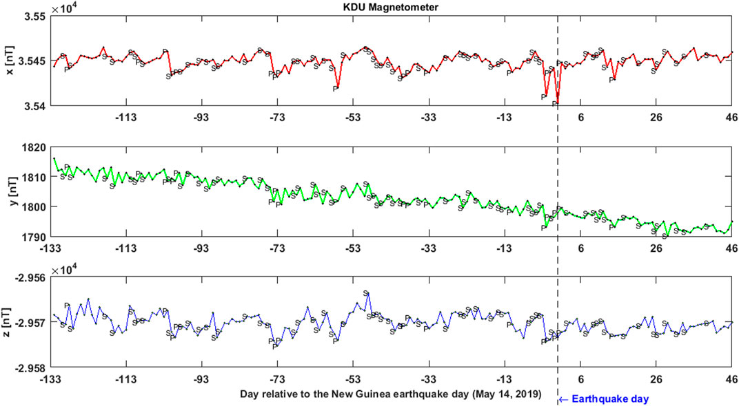
FIGURE 3. KDU magnetometer (12.69°S, 132.47°E) measurements (A) x, (B) y, and (C) z during the period from January 01 to June 30, 2019. The earthquake day is indicated by a dashed black vertical line.

Swarm-TEC Data

The size of the affected area by an impending earthquake can be estimated with the formula $R={10}^{0.43M},$ where R is the radius in kilometers of the earthquake preparation zone, supposed circular and centered at the earthquake epicenter, and M is its magnitude (Dobrovolsky et al., 1979). Therefore, to detect the potentially seismo-ionospheric anomalies, we only considered all tracks of satellites A, B, and C crossing the Dobrovolsky’s region, i.e., within R ∼ 1,850 km from the New Guinea earthquake epicenter during the period of January 01 to June 30, 2019.

For every day, the median of the VTEC values in Dobrovolsky’s area was calculated and, finally, the time series of the median values were constructed. Due to the nonlinear variations of VTEC, a polynomial of degree 4 was fitted to the time series and the residuals between the two curves were considered as a new time series. For convenience, we will still use the name VTEC for the y-axis but we are adding the term “detrend” to intend that actually, what is plotted is the VTEC detrended by the polynomial fit.

Figure 4, Supplementary Figures S1, S2 show the night-time VTEC residual variations of Swarm A, B, and C satellites during the period from January 01 to 30 June 30, 2019, respectively. The abscissa indicates the day relative to the earthquake day. The vertical dotted line represents the earthquake date. Median higher and lower bounds are drawn as blue and green horizontal lines, respectively. The pre-defined allowed ranges are $\mathit{m}\pm 1.5\times \mathit{Iqr}$ in which m and Iqr are the median and the inter-quartile range statistical parameters, respectively. In the case of Gaussian residuals, this threshold would correspond to around two times the standard deviation from the mean. In this figure, the perturbed days with high geomagnetic activities are shown with the “P” symbol (“P” stands for “perturbed”) and the ones with high solar activity are shown with the “S” symbol (“S” stands for “solar”). It should be noted that the values of the median and the allowed bounds were calculated using only the quiet geomagnetic days (i.e., those points without “P” indication), taking into account the magnetic indices, F10.7, and the ACE solar wind parameters.

FIGURE 4

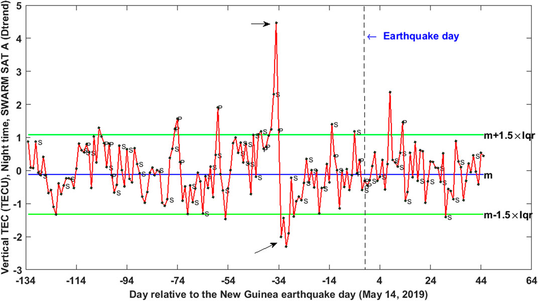
FIGURE 4. Results of Swarm A night time VTEC data analysis for the Papua New Guinea (May 14, 2019) from January 01 to June 30, 2019. The symbols “P” and “S” indicate disturbed magnetic days (“P” according to magnetic indices, “S” according to solar parameters).

Figure 4 shows a striking anomaly when the VTEC night-time variations measured by Swarm A exceed the higher bound with the value of 311.03%, 35 days before event. This time series indicates other unusual variations 4, 13, and 31 days before the earthquake with the deviation values of 8.27%, 29.32%, and −74.68%, respectively. The VTEC night-time variations measured by Swarm C acknowledge the observed anomalies by Swarm A on 31 and 35 days prior to the earthquake (Supplementary Figure S1).

Supplementary Figure S2 regards the VTEC parameter measured by Swarm B in night time: it shows the gradual and abnormal increase from about 23 days before the earthquake that descends 3 days before the earthquake and reaches its lowest level around the earthquake day. VTEC variations exceed the lower bound with the value of 19.19%, 1 day before the earthquake during normal solar and geomagnetic activity.

It is observed that the anomalous value of the VTEC parameter on the day of the earthquake coincides with the high geomagnetic activity on this day (Figure 2) and we encounter a complex situation. Two days present significant anomalies preceding 13 and 7 days of the earthquake occurrence with the values of 26.90% and 48.33% above the threshold, respectively. Also, the night-time VTEC values on 20 and 23 days before the earthquake slightly exceed the upper boundary.

It seems that from 23 to 7 days, there are some spots–increase of the oscillation of electron content in the ionosphere–mainly toward positive values overpassing the threshold, and on the day before the earthquake, there is a precipitation of electrons in the lower layers of the same ionosphere or the chemical composition of the ionosphere changed and so enhanced the recombination rate. Even if we propose a link of this depletion of electrons with the impending earthquake, we need to note that it happened between two geomagnetically disturbed periods, so even an external perturbation of the ionosphere can be the source of this phenomenon. Supplementary Figure S3 shows the Swarm B satellite day-time VTEC residual variations during the period of January 01 to June 30, 2019. This figure confirms the anomalous VTEC variations on 20 days preceding the earthquake when VTEC exceeds the upper bound with the value of 90.59%.

Swarm Magnetic Field Anomalies

In order to make a comparative analyses, six other parameters measured by satellites A, B, and C including scalar and vectors’ (X, Y, Z) magnetic components, electron density, and electron temperature were analyzed during the period from January 01 to June 30, 2019, inside the Dobrovolsky’s area.

For anomaly detection in the magnetic field components, at the first step, the difference between the measured parameter in nominal satellite conditions and the predicted value using the IGRF-12 (International Geomagnetic Reference Field) (Thébault, et al., 2015) model was computed. Afterwards, the median of the residuals of magnetic values of each track inside the Dobrovolsky’s area separately for day and night was calculated and finally, the time series of the magnetic field median values during the period from January 01 to June 30, 2019 was created. It should be noted that to obtain residual curves of magnetic components using the IGRF model, all tracks of Swarm satellite inside a square centered in earthquake epicenter with a diagonal equals to two times of Dobrovolsky’s radius were considered (the use of a square instead of a circular area of investigation was motivated to have analyzed tracks with the same length). To remove the seasonal variations and all variations not predicted by the IGRF, a polynomial of degree 4 was fitted to the time series and the residual values were finally calculated. A threshold value is defined as $\mathit{ m}\pm 1.50\times \mathit{Iqr}$. Therefore, we select those residual values of the observed parameter if they exceed the pre-defined threshold in geomagnetically quiet conditions (|Dst| ≤ 20 nT, a_p < 25 nT and F10.7 < 120). Further checking of the identified anomalies is made that also takes into account the external conditions evaluated by IMF and solar wind speed as specified in 2.1 “Solar and geomagnetic data” section. The final selected anomalies are then regarded as an anomaly candidate, i.e., a potential seismic anomaly.

Figure 5 illustrates the day-time Y magnetic field values measured by satellite B during the study period. Striking anomalies are seen on 26, 20, and 7 days and 1 day before the earthquake occurrence with the values of 11.22%, −42.45%, −8.55%, and −25.77% of the allowable bounds in geomagnetically quiet conditions, respectively. The Swarm Bravo magnetic Y component time series during night time is not shown as it does not contain any apparent anomaly.

FIGURE 5

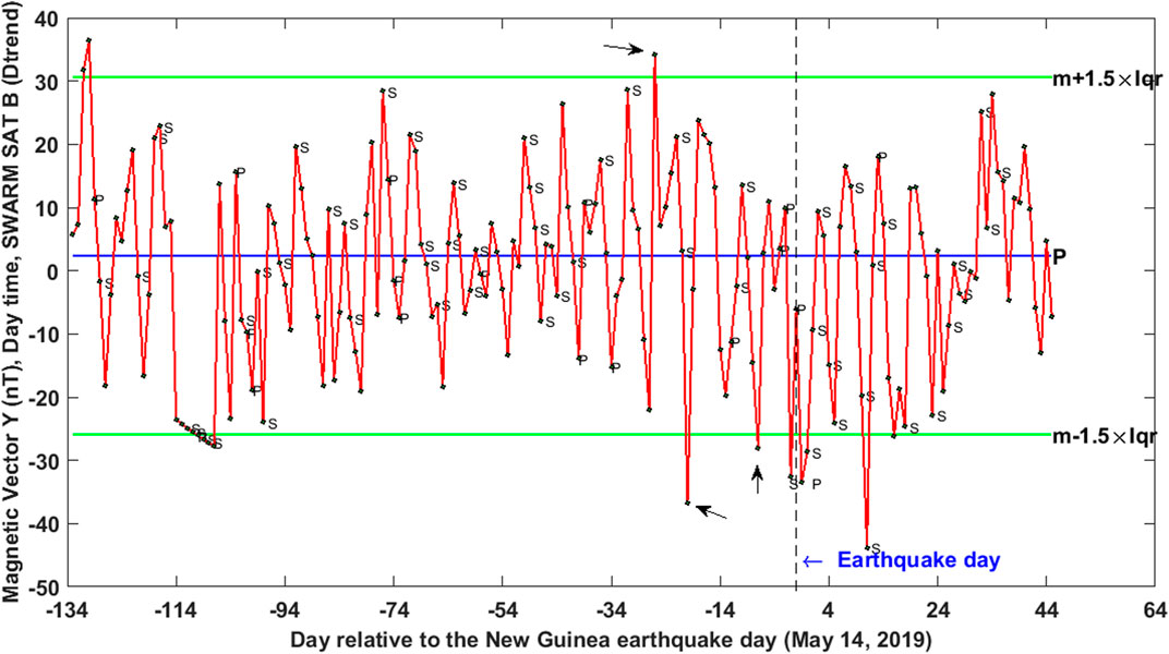
FIGURE 5. Results of Y magnetic field data analysis from Swarm B for the New Guinea earthquake (May 14, 2019) from January 01, to June 30, 2019 at day time. The symbols “P” and “S” indicate disturbed magnetic days (“P” according to magnetic indices, “S” according to solar parameters).

Figure 6A presents the recorded track of satellite B close to the New Guinea earthquake epicenter on 14 May, half an hour before the earthquake time. The residual of the time series of the first derivatives of the measured magnetic fields scalar and vectors (X, Y, Z) values and a cubic spline are shown in Figures 6A–D, respectively. The vertical axis represents the geomagnetic latitude. An unusual variation in the time series of the residual curve of the X, Y, and Z components of the magnetic field is clearly seen around the earthquake location (the red arrows in Figure 6). We note another smaller perturbation in the southern position but, with respect to the underlined one, it is very short, and it is probably due to moderate geomagnetic activity.

FIGURE 6

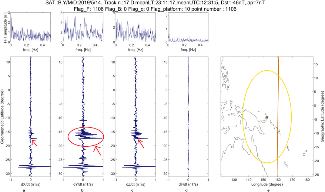
FIGURE 6. Results of Swarm B track analysis for the New Guinea earthquake (May 14, 2019) on earthquake day. (E) A map of the region with the longitude in horizontal axis and latitude in vertical one is represented. A green asterisk, a brown line, and a yellow circle represent the earthquake epicenter, the track, and Dobrovolsky’s area, respectively. The track crossed the Dobrovolsky’s area between the 12:27:12 and 12:35:03 UTC. (A–D) The residuals of the time series of the derivatives of the measured scalar magnetic field (X, Y, Z) components and F, respectively, along this track. The vertical axis represents the geomagnetic latitude. Above each analysis, the FFT spectra are represented too.

Supplementary Figure S4 shows the track of satellite B crossing the Dobrovolsky’s area 20 days before the main shock. Anomalous variations are clearly seen in the time series of the residual curves of the vectors X, Y, and Z of the magnetic field around the earthquake location.

We noted that the Y component is a little more disturbed than X and Z for anomalies depicted in Figure 6 and Supplementary Figure S4.

Although the time series analysis does not underline any anomaly in the mean night-time Y daily values of magnetic field, a single track analysis shows some anomalies also in this period. Figure 7 and Supplementary Figure S5 show the two candidates of pre-earthquake anomalies that preceded the main seismic event by about 2 days and 1 month. Both tracks were acquired during geomagnetic quiet conditions and show a clear anomaly around the future epicentral coordinates (indicated by a red circle). The FFT of Y component of Figure 7 shows a peak centered at a frequency of 0.13 Hz that corresponds to a period of 7.4 s. In Supplementary Figure S5, the identified anomaly is more evident in the Y component, supporting the hypothesis of an internal source for this signal. It is worth noting that the epicentral latitude corresponds to the southern peak of the equatorial ionospheric anomaly (EIA): this implies that we cannot completely exclude that the underlined anomalies are intrinsic phenomena of the ionospheric response to the solar diurnal activity. However, in the cases shown in Figure 7 and Supplementary Figure S5, the night local time would exclude a typical EIA on that occasion: these anomalies are also called absolute ionospheric precursors (Pulinets and Ouzounov, 2018). In addition, all other tracks did not show these kinds of anomalies at −15° of geomagnetic latitude, deposing more for a transient phenomenon in the two cases shown in Figure 7 and Supplementary Figure S5.

FIGURE 7

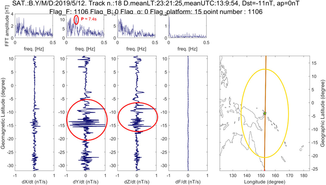
FIGURE 7. Swarm B night-time data analysis of the track that preceded the earthquake by about 2 days (−1.99 days). The same elements of Figure 8 are shown, and, in addition, the FFT of the signal inside the Dobrovolsky area is reported for each magnetic field component and total intensity. For Y magnetic field component, the FFT evidences a peak at 7.4 s.

Supplementary Figure S6 shows the night-time Z magnetic field values measured by satellite B during the study period. Unusual variation is seen on 29 days before the event with the values of 3.12% of the higher bound in geomagnetically quiet conditions.

Supplementary Figures S7 illustrates the night-time Y magnetic field values measured by satellite C. Clear anomaly is seen on 5 days before the event with the values of 5.36% of the higher bound in geomagnetically quiet conditions; nevertheless, it presents some solar activity, so its origin could be likely due to an external source, i.e., the Sun.

Swarm Electron Density and Temperature Anomalies

For every track inside the Dobrovolsky’s area at every day, the median of each parameter including the electron density and the electron temperature separately for day and night were obtained and finally, the time series of the median values, for day and night during the studied period, were created. However, since the variations of the plasma parameters are affected by nonlinear variations, a polynomial of degree 4 fitted to the time series and the residuals between the two curves as a new time series was calculated.

Figure 8 and Supplementary Figure S8 show the Swarm A satellite electron density residual variations during the period from January 01 to June 30, 2019 for night and day times. Two striking anomalies are seen on 32 and 35 days before the event when the parameter variations exceed the higher bound with the values of 229.84% and 236.21%, respectively.

FIGURE 8

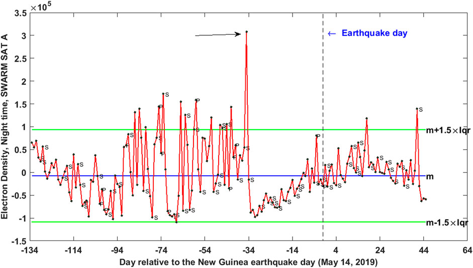
FIGURE 8. Results of Swarm A electron density data analysis for the New Guinea earthquake (May 14, 2019) from January 01 to June 30, 2019 at night time. The symbols “P” and “S” indicate disturbed magnetic days (“P” according to magnetic indices, “S” according to solar parameters).

Supplementary Figure S9 shows the Swarm B satellite night-time electron density residual variations during the period of January 01 to June 30, 2019.

It is interesting that this figure confirms the results deduced from Supplementary Figure S2, which indicated night-time VTEC variations. It is seen that electron density variations encounter with a rising trend from about 20 days before the event and then fall in day earthquake similar to VTEC variations. It exceeds the upper bound on −7 days before the earthquake with a value of 253.42%.

Figure 9 shows the track of satellite B on 7 days before the earthquake (May 07) inside the Dobrovolsky’s area. To look for possible seismo-anomalies, a polynomial of degree 12 along this track has been fitted and subtracted. The residuals of the measured electron density/temperature are shown in Figures 9B,C. The vertical axis represents the geomagnetic latitude. Unusual variations of the electron density and electron temperature in the residual time series are clearly seen close to the earthquake location (the red arrows in Figure 9).

FIGURE 9

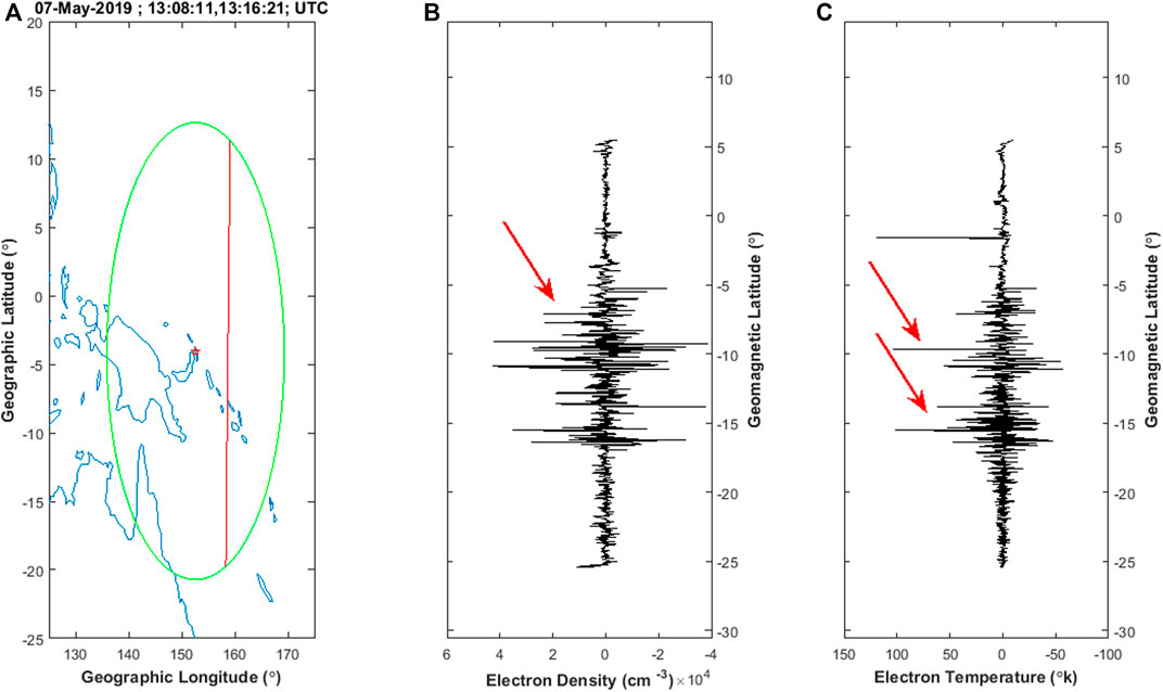
FIGURE 9. Results of Swarm B track analysis for the New Guinea earthquake (May 7 , 2019), 7 days before earthquake day. (A) A map of the region with the longitude in the horizontal axis and latitude in vertical one is represented. A red asterisk, a brown line, and a yellow circle represent the earthquake epicenter, the track, and Dobrovolsky’s area, respectively. The track crossed the Dobrovolsky’s area between the 13:08:11 and 13:16:21 UTC. (B,C) show the differences between the time series of the measured electron density and temperature and a polynomial of degree 20 fitted along the same track. The vertical axis represents the geomagnetic latitude.

It should be noted that the detected anomalies in the measured parameters using Swarm A can be compared by the corresponding measured parameters in Swarm C due to the same orbit altitude and also the close distance (about 1.4° longitudinal separation) between two satellites. For this reason, we decided to apply a similar technique used by Zaxapros et al. (2019) to study the variation of Ne associated with a typhoon in Pacific Ocean. Figure 10 and Supplementary Figure S10 show the variations of differences between gradients of electron density values measured by Swarm A and C at night and day, respectively, clear anomalies are seen on 34 days before the event.

FIGURE 10

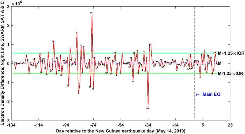
FIGURE 10. Differences between gradients of electron density values measured by Swarm A and C from January 01 to June 30, 2019 at night time. The symbols “P” and “S” indicate disturbed magnetic days (“P” according to magnetic indices, “S” according to solar parameters).

Supplementary Figure S11 shows the Swarm C satellite night-time electron temperature residual variations during the period from January 01 to June 30, 2019. It is interesting that the latter figure confirms the results deduced from Swarm A. Clear anomalies are seen between 20 and 32 days before the earthquake, especially on 30 days prior to the event with a value of 179.84%.

CSES Satellite Data Analysis

As we noticed that in the analyses of the electron density, some trends still remain that could be due to the Swarm local time precession, we decided to perform a similar analysis with the data from China Seismo-Electromagnetic Satellite (CSES, also known as CSES-01 or Zhangheng-01) that has a fixed local time at ∼2:00 a.m. for night time and ∼2:00 p.m. for day time (Shen et al., 2018). The median electron density of the samples acquired inside the Dobrovolsky’s area during only geomagnetic quiet time (|Dst| ≤ 20 nT and a_p ≤ 10 nT) have been computed separately for day-time tracks and night-time tracks. The seasonal trend has been removed by a 3rd degree and 7th degree polynomial for night and day time, respectively. Figures 11, 12 show the residual trends for night and day time as well as the median values plus or minus 1.5 times the interquartile range of the same series. The points outside the given threshold, i.e., the anomalous ones, have been underlined by datatips with the indication of the day with respect to the earthquake and the residual value of electron density in e⁻/cm³.

FIGURE 11

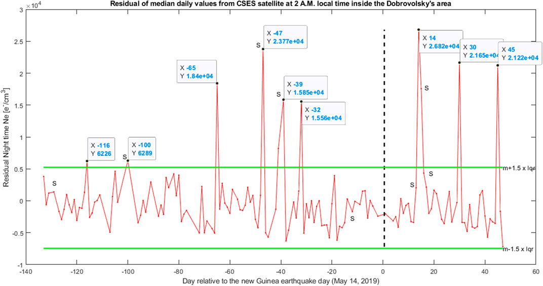
FIGURE 11. CSES daily median electron density during night time (2:00 a.m.). Only data acquired during geomagnetic quiet time (|Dst| ≤ 20 nT and a_p ≤ 10 nT) has been shown. Days with high solar activity are depicted by “S.”

FIGURE 12

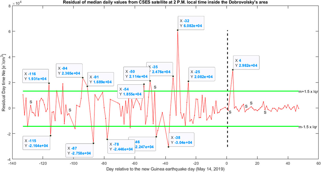
FIGURE 12. CSES daily median electron density during day time (2:00 p.m.). Only data acquired during geomagnetic quiet time (|Dst| ≤ 20 nT and a_p ≤ 10 nT) has been shown. Days with high solar activity are depicted by “S.”

Discussion

The characteristics and temporal evolution of the detected anomalies in the variations of discussed parameters are listed in Table 1. This table shows the day of anomaly occurrence with respect to the earthquake, the night or day local time, and the anomaly value with respect to the median; all the anomalies are identified in quiet geomagnetic times, i.e., when the geomagnetic indices and the solar activity, as detected by ACE, were both low. The same day can be indicated with and without solar activity because we take into account the specific time that the satellite crossed the Dobrovolsky area and the solar activity can change during the day. In this table, only the positive anomalies of TEC and electron density have been listed because the earthquakes are expected to increase the ionospheric electron density (e.g., He and Heki, 2017 with the model described by Enomoto, 2012). In general, it appears that electron density and VTEC are the most sensitive quantities to the earthquake preparation phase (both with 20 anomalies before the earthquake occurrence), while the magnetic field is the least sensitive (only 7 anomalies).

TABLE 1

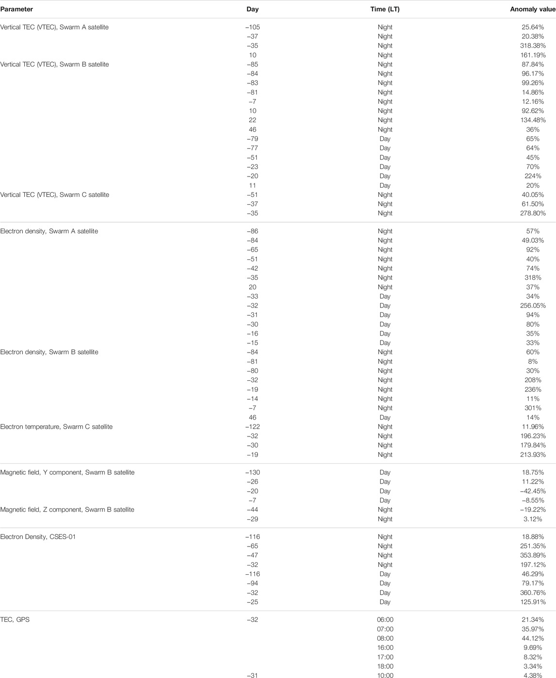
TABLE 1. A summary of the detected anomalies in the investigated period. The anomalies are sorted following these criteria: satellite that detects, night and day, before and after the earthquake occurrence, and finally, in chronological order. The anomalies detected during high magnetic or solar activity are not listed. Also, TEC and Ne negative anomalies are not included.

We noted that the local time of Swarm Alpha and Charlie around 34 days before the earthquake was close to sunrise and sunset (6:00 a.m. and 6:00 p.m., respectively). So, the anomalies (especially in VTEC and Ne) recorded around this day need to be further discussed to understand better if their origin could be linked to the local time of the satellite or real special ionospheric conditions. A further analysis made use of TEC recorded by the ground station for 24 h on the day, presented in the following paragraph that will address this issue.

Figure 13A shows GNSS-TEC variations deduced from GIM data and the closest grid node (5^°S, 150^°E) to the epicenter during the period from April 01 to June 30, 2019. Unusual GNSS-TEC variations are sharply seen on 32 and 31 days prior to the earthquake. Figure 13B shows variations of DTEC $\left(DTEC=\frac{TEC-Median}{Interquartile}\right)$. Figure 13C shows anomalous TEC values detected using the median method when $\left|DTEC\right|>1.5$. After considering only quiet solar and geomagnetic conditions (ap < 25 nT, |Dst| ≤ 20 nT, and F10.7 < 120 SFU), Figure 13D indicates striking TEC anomalies 32 days before the event between 06:00 and 08:00 UTC and also between 16:00 and 18:00 UTC. The DTEC value has an increase of the order of 44.12%, from the normal state at 08:00 UTC.

FIGURE 13

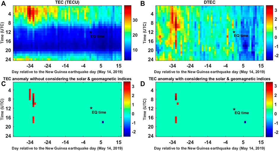
FIGURE 13. Summary of TEC analysis results using median method for the Papua New Guinea (May 14, 2019) from April 01 to June 30, 2019. The y-axis represents the time UTC (LT = UTC − 5:00). (A) TEC variations, (B) DTEC variations calculated by formula of $DTEC=\frac{TEC-Median}{Interquartile}$, (C) detected TEC anomalies when |DTEC| = > 1.5, and (D) detected TEC anomalies when ap < 20 nT, $\text{Dst }>-20\text{ nT}$, Dst < 20 nT and F10.7 < 120, and ∼|DTEC| = > 1.5.

From this analysis, it is evident that the anomaly recorded 31 days before the earthquake occurrence is not an artefact of the local time covered by Swarm as the ground station has a full coverage. From Figure 13A, we can even infer that the recorded TEC anomalies are mainly an increase of the crests of the equatorial ionospheric anomalies that is a phenomenon that has been previously found for several earthquakes mainly by the DEMETER satellite (e.g., Li and Parrot, 2012).

A final check of the most anomalous day in night Swarm Bravo VTEC data before the earthquake occurrence is presented. Figure 14 shows the TEC map around the earthquake on May 7, 2019 at 13:00 UTC. The Swarm Bravo track projections have been displayed over by red lines and the right one between 13:06 and 13:17 UTC is the one where the GNSS Swarm receiver found the VTEC anomaly of the May 7, 2019. The map confirms that inside the Dobrovolsky, there is an enhancement of TEC as seen by Swarm B VTEC. Moreover, the map also shows that the TEC anomaly is well inside the Dobrovolsky area and with this highest value close to the future epicenter (a bit shifted North-East).

FIGURE 14

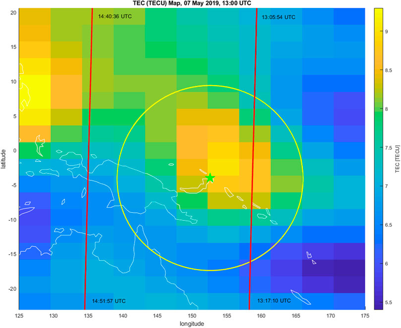
FIGURE 14. TEC map around the M7.6 Papua New Guinea (May 14, 2019) earthquake on May 7, 2019 at 13:00 UTC. The epicenter is represented as a green star; its Dobrovolsky area is shown by a yellow circle. The red lines represent the Swarm Bravo projection of the track in the same area and time.

We noticed that the most anomalous VTEC value occurred 35 days before the earthquake, as expected for the strict physical link between TEC and Ne; in the same day also, the in situ electron density shows an anomalous increase of its value. Furthermore, this anticipation time is very close to the ones found for an increase of electron density before the M7.5 Indonesia 2018 (40 days) and M7.1 California Ridgecrest 2019 (33 days) earthquakes (Marchetti et al., 2019b; De Santis et al., 2020). It is interesting to note that these events have a similar earthquake magnitude, and one of them even occurred in different region/tectonic settings (i.e., Ridgecrest). So, it would be interesting in future studies to further verify whether the ionosphere could respond 30–40 days before earthquakes with this magnitude. This fact would confirm the validity of Rikitake law (1987) as recently established also for satellites by De Santis et al. (2019).

The sequence of all anomalies, taken from all Swarm satellite observables (i.e., VTEC, electron density, electron temperature, and Y, Z magnetic field components) has been finally considered in their whole by constructing the cumulative number of anomalous days. The anomalies that are due to an increase of solar activity checked on the data measured by the ACE satellite from 2 h before the anomaly to its occurrence have been excluded from this cumulate. If the ionospheric anomaly preceded the IMF ones it is not excluded as the magnetosphere coupling can be immediate or needs some delay that the solar wind can impact the ionosphere from the observation point of ACE (about 1.4 millions of kilometers away from Earth) but not precede. Figure 15 shows the cumulative number of anomalous days with respect to the day of the earthquake (here placed as time zero), weighting each anomalous day for the same unitary amount. The dark- and light-gray curves are two sigmoidal (Boltzmann) fits over two distinct parts of the points (see Figure 15; the first fit is partial for the early analyzed period, while the second one comprises some data before and after the earthquake occurrence), the linear fit is given by a dashed (oblique) line, over all detected anomalies. It is evident that there are two accelerations of anomalies before the earthquake, and for this reason the data have been divided into two time intervals separated at −77 days. The two intervals have been fitted by sigmoidal curves shown in light and dark gray with adjusted R² = 0.980 and R² = 0.992 (both are better than the linear fit with R² = 0.958). The second curve, i.e., the one from −77 to +60 days with respect to the earthquake day, is the one with better statistical indications, and it indicates a turning point of the system (the inflection point of the full sigmoidal curve indicated as vertical dashed black line) at about −29 days, i.e., the ionosphere showed a critical behavior about 1 month before the mainshock. Furthermore, a first increase of anomaly has been depicted at about 80 days before the earthquake and this seems to be a typical anticipation time for ionospheric disturbances as extensively (on more than 1,000 earthquakes) analyzed by De Santis et al. (2019).

FIGURE 15

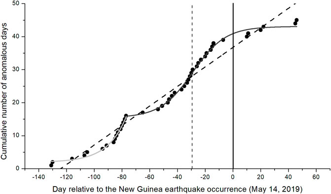
FIGURE 15. Cumulative number of anomalous days (considering all the Swarm satellites and presented time series) with respect to the day of occurrence of the Papua New Guinea mainshock (negative days before the earthquake occurrence, positive after). Anomalies are shown as black circles, while dark- and light-gray curves are sigmoidal (Boltzmann) fits over two subsequent intervals; the dashed line is the linear fit. The vertical black line is the time of the earthquake, while the vertical dashed line is the inflection of the sigmoidal dark-gray curve.

A confutation analysis was finally performed to acknowledge the potentially detected anomalies in VTEC variations measured by Swarm B. Supplementary Figure S12 shows the results of Swarm B night time VTEC data analysis for the location of 4.051^°S, 85^°E, outside the Doborovolsky’s area from January 01 to June 30, 2019. According to the USGS catalogue, no significant (M > 6) earthquake was recorded in this area during the analyzed time. Some minor events have been localized, in particular an M6.0 on February 02, 2019 and its aftershocks, but we underline that such events are not significant when compared with the tectonic of the region that potentially can generate M7.5+, or even greater events, as it is in the interaction plate boundary between Sunda and Indian plates. In addition, no Swarm anomalies are seen from about 100 days before the main event to the earthquake occurrence day, providing evidences that the identified anomalies for Papua New Guinea are confined inside the Dobrovolsky’s area.

Therefore the all of implemented comparative and confutation analyses, reduce the uncertainty about the source of the observed anomalies and lead to make a robust decision about the observed anomalies in VTEC time series measured using Swarm satellites.

Conclusion

This paper presents the first study concerning the Swarm-TEC data analysis to detect seismo-ionospheric anomalies. In order to make some robust comparative analyses, other six measured plasma and magnetic field parameters from Swarm satellites and GNSS-TEC measurements were also investigated, together with the electron density of CSES. Results show clear anomalies on the earthquake day and some days before the main seismic event, with significant concentrations (acceleration) of anomalies on around 80 and 30 days before the mainshock. We were careful to detect the anomalies during low geomagnetic activity, so those anomalies could be considered potentially as pre-seismic anomalies. Interesting enough, we find that a sigmoidal fit represents well the behavior of part or all anomalies toward the time of main earthquake occurrence: in particular, the sigmoid closer to the earthquake occurrence shows the inflection point about 1 month before the earthquake, supporting an underlying critical system pointing toward a critical point. Moreover, the electron density variations acknowledge the VTEC variations, better supporting the found results. Our finding shows that, for the present case study, the magnetic field component Y appears to be the most sensitive component to ionospheric anomalies with respect to X, Z, and total intensity but the least one with respect to the other analyzed ionospheric parameters.

Therefore, Swarm-TEC measurements could be used as one of the main data sources for studies on earthquake precursors, especially in combination with electron density and magnetic field in situ satellite observations. This reinforces the multi-precursors analysis, which remains the most favored approach to study the preparation phase of large earthquakes with non-seismic data.

Data Availability Statement

Publicly available datasets were analyzed in this study. This data can be found in the following: The European Space Agency (ESA) for the Swarm data at HTTP or FTP (anonymous login) server: swarm-diss.eo.esa.int, NASA NOAA for the solar and geomagnetic indices at https://www.ngdc.noaa.gov/geomag/indices/indices.html. The China Earthquake Administration, China National Space Administration and Italian Space Agency for the data of CSES-01 available upon request and formal approval at www.leos.ac.cn. Ground magnetic field measurements are freely available at www.intermagnet.org.

Author Contributions

MA, AD, DM, and XS: Conceptualization, Methodology, Software. MA, AD, and DM: Data curation, Writing-Original draft preparation, Writing- Reviewing and Editing.

Funding

Part of this work has been funded by the SAFE (Swarm for Earthquake Study) project (ESA) and by LIMADOU-Science+ Project (Italian Space Agency). Partial funds were also provided by FURTHER (INGV) Project, “Pianeta Dinamico-Working Earth” Project (Italian Ministry of University and Research—project code: D53J19000170001), “Research on anomaly extraction technology of seismic electromagnetic satellite data based on blind source separation” project (National Natural Science Foundation of China, Grant number 41974084), and project “Research on multiparametric anomalies in Lithosphere-Atmosphere-Ionosphere before the earthquakes” (Grant number: 2021M691190) funded by the China Postdoctoral Science Foundation.

Conflict of Interest

The authors declare that the research was conducted in the absence of any commercial or financial relationships that could be construed as a potential conflict of interest.

Publisher’s Note

All claims expressed in this article are solely those of the authors and do not necessarily represent those of their affiliated organizations, or those of the publisher, the editors and the reviewers. Any product that may be evaluated in this article, or claim that may be made by its manufacturer, is not guaranteed or endorsed by the publisher.

Acknowledgments

The authors would like to acknowledge the European Space Agency (ESA) for the Swarm data, NASA Jet Propulsion Laboratory for the solar and geomagnetic indices. We also thank “Geoscience Australia (GA)”, for supporting its operation and INTERMAGNET for promoting high standards of magnetic observatory practice (www.intermagnet.org). Some of the results presented in this paper rely on the data collected at “Kakadu.”

Supplementary Material

The Supplementary Material for this article can be found online at: https://www.frontiersin.org/articles/10.3389/feart.2022.820189/full#supplementary-material

Footnotes

¹Swarm Expert Support Laboratories Swarm L2 TEC Product Description, Doc. No. SW-TR-GFZ-GS-0007, Rev:4, 2017-05-22.

²Swarm Level 2 Processing Facility Product specification for L2 Products and Auxiliary Products (SW-DS-DTU-GS-0001).

References

Akhoondzadeh, M., Parrot, M., and Saradjian, M. R. (2010). Electron and Ion Density Variations Before Strong Earthquakes (M>6.0) Using DEMETER and GPS Data. Nat. Hazards Earth Syst. Sci. 10, 7–18. doi:10.5194/nhess-10-7-2010

CrossRef Full Text | Google Scholar

Akhoondzadeh, M., De Santis, A., Marchetti, D., Piscini, A., and Cianchini, G. (2018). Multi Precursors Analysis Associated with the Powerful Ecuador (MW= 7.8) Earthquake of 16 April 2016 Using Swarm Satellites Data in Conjunction with Other Multi-Platform Satellite and Ground Data. Adv. Space Res. 61, 248–263. doi:10.1016/j.asr.2017.07.014

CrossRef Full Text | Google Scholar

Akhoondzadeh, M., De Santis, A., Marchetti, D., Piscini, A., and Jin, S. (2019). Anomalous Seismo-LAI Variations Potentially Associated with the 2017 Mw = 7.3 Sarpol-E Zahab (Iran) Earthquake from Swarm Satellites, GPS-TEC and Climatological Data. Adv. Space Res. 64, 143–158. doi:10.1016/j.asr.2019.03.020

CrossRef Full Text | Google Scholar

Chen, K., Milliner, C., and Avouac, J. P. (2019). The Weitin Fault, Papua New Guinea, Ruptured Twice by M W 8.0 and M W 7.7 Earthquakes in 2000 and 2019. Geophys. Res. Lett. 46, 12833. 833–12,840, 12840. doi:10.1029/2019GL084645

CrossRef Full Text | Google Scholar

Cianchini, G., De Santis, A., Di Giovambattista, R., Abbattista, C., Amoruso, L., Campuzano, S. A., et al. (2020). Revised Accelerated Moment Release under Test: Fourteen Worldwide Real Case Studies in 2014–2018 and Simulations. Pure Appl.Geoph. 177 (9), 4057–4087. doi:10.1007/s00024-020-02461-9

CrossRef Full Text | Google Scholar

De Santis, A., Balasis, G., Pavón-Carrasco, F. J., Cianchini, G., and Mandea, M. (2017). Potential Earthquake Precursory Pattern from Space: the 2015 Nepal Event as Seen by Magnetic Swarm Satellites. Earth Planet. Sci. Lett. 461, 119–126. doi:10.1016/j.epsl.2016.12.037

CrossRef Full Text | Google Scholar

De Santis, A., Cianchini, G., Marchetti, D., Piscini, A., Sabbagh, D., Perrone, L., et al. (2020). A Multiparametric Approach to Study the Preparation Phase of the 2019 M7.1 Ridgecrest (California, United States) Earthquake. Front. Earth Sci., 8. doi:10.3389/feart.2020.540398

CrossRef Full Text | Google Scholar

De Santis, A., De Franceschi, G., Spogli, L., Perrone, L., Alfonsi, L., Qamili, E., et al. (2015). Geospace Perturbations Induced by the Earth: the State of the Art and Future Trends. Phys. Chem. Earth, Parts A/B/C 85-86, 17–33. doi:10.1016/j.pce.2015.05.004

CrossRef Full Text | Google Scholar

De Santis, A., Marchetti, D., Pavón-Carrasco, F. J., Cianchini, G., Perrone, L., Abbattista, C., et al. (2019). Precursory Worldwide Signatures of Earthquake Occurrences on Swarm Satellite Data. Sci. Rep. 9, 20287. doi:10.1038/s41598-019-56599-1

PubMed Abstract | CrossRef Full Text | Google Scholar

Dobrovolsky, I. P., Zubkov, S. I., and Miachkin, V. I. (1979). Estimation of the Size of Earthquake Preparation Zones. Pageoph 117, 1025–1044. doi:10.1007/bf00876083

CrossRef Full Text | Google Scholar

Enomoto, Y. (2012). Coupled Interaction of Earthquake Nucleation With Deep Earth Gases: A Possible Mechanism for Seismo-Electromagnetic Phenomena. Geophys. 191 (3), 1210–1214. doi:10.1111/j.1365-246X.2012.05702.x

CrossRef Full Text | Google Scholar

Foelsche, U., and Kirchengast, G. (2002). A Simple "geometric" Mapping Function for the Hydrostatic Delay at Radio Frequencies and Assessment of its Performance. Geophys. Res. Lett. 29 (10), 111–1. doi:10.1029/2001GL013744

CrossRef Full Text | Google Scholar

Freund, F. (2009). Stress-activated Positive Hole Charge Carriers in Rocks and the Generation of Pre-earthquake Signals. In Electromagnetic Phenomena Associated with Earthquakes, Ed. By M. Hayakawa, Transworld Research Network, Trivandrum, 41–96.

Google Scholar

Friis-Christensen, E., Lühr, H., and Hulot, G. (2006). Swarm: A Constellation to Study the Earth’s Magneticfield. Earth Planets Space 58, 351–358. doi:10.1186/BF03351933

CrossRef Full Text | Google Scholar

Geller, R. J. (1997). Earthquake Prediction: a Critical Review. Geoph. J. Inter. 131 (3), 425–450. doi:10.1111/j.1365-246x.1997.tb06588.x

CrossRef Full Text | Google Scholar

Guo, J., Li, W., Liu, X., Wang, J., Chang, X., and Zhao, C. (2015). On TEC Anomalies as Precursor Before MW 8.6 Sumatra Earthquake and MW 6.7 Mexico Earthquake on April 11, 2012. Geosci. J. 19, 721–730. doi:10.1007/s12303-015-0005-6

CrossRef Full Text | Google Scholar

Haagmans, R., Bock, R., and Rider, H. (2013). Swarm; ESA’s Magnetic Field mission. Available at: https://earth.esa.int/documents/700255/1805948/ESA+magnetic+field+mission/36942f02-b2d4-4787-af81-eb19efb74265.

Google Scholar

Hayakawa, M., and Molchanov, O. A. (2002). Seismo- Electromagnetics: Lithosphere-Atmosphere-Ionosphere Coupling. Tokyo: Terra Scientific Publishing Co, 477.

Google Scholar

He, L., and Heki, K. (2017). Ionospheric anomalies immediately before Mw 7.0–8.0 earthquakes. J. Geophys. Res. Space Phys. 122, 8659–8678. doi:10.1002/2017JA024012

CrossRef Full Text | Google Scholar

Li, M., and Parrot, M. (2012). Real Time Analysis of the Ion Density Measured by the Satellite DEMETER in Relation With the Seismic Activity. Nat. Hazards Earth Syst. Sci. 12, 2957–2963. doi:10.5194/nhess-12-2957-2012

CrossRef Full Text | Google Scholar

Liu, J. Y. (2018). “Seismo-ionospheric Precursors of the 2017 M7.3 Iran-Iraq Border Earthquake and the 2018 M5.9 Osaka Earthquake Observed by FORMOSAT-5/AIP,” in EMSEV 2018, International Workshop Integrating Geophysical Observations from Ground to Space for Earthquake and Volcano Investigations Potenza (Basilicata: Italy), 17–21.

Google Scholar

Marchetti, D., and Akhoondzadeh, M. (2018). Analysis of Swarm Satellites Data Showing Seismo-Ionospheric Anomalies Around the Time of the strong Mexico (Mw = 8.2) Earthquake of 08 September 2017. Adv. Space Res. 62, 614–623. doi:10.1016/j.asr.2018.04.043

CrossRef Full Text | Google Scholar

Marchetti, D., De Santis, A., D'Arcangelo, S., Poggio, F., Piscini, A., A. Campuzano, S., et al. (2019a). Pre-earthquake Chain Processes Detected from Ground to Satellite Altitude in Preparation of the 2016-2017 Seismic Sequence in Central Italy. Remote Sensing Environ. 229, 93–99. doi:10.1016/j.rse.2019.04.033

CrossRef Full Text | Google Scholar

Marchetti, D., De Santis, A., Shen, X., Campuzano, S. A., Perrone, L., Piscini, A., et al. (2020b). Possible Lithosphere-Atmosphere-Ionosphere Coupling Effects Prior to the 2018 Mw = 7.5 Indonesia Earthquake from Seismic, Atmospheric and Ionospheric Data. J. Asian Earth Sci. 188, 104097. In Press. doi:10.1016/j.jseaes.2019.104097

CrossRef Full Text | Google Scholar

Marchitelli, V., Harabaglia, P., Troise, C., and De Natale, G. (2020). On the Correlation between Solar Activity and Large Earthquakes Worldwide. Sci. Rep. 10, 11495. doi:10.1038/s41598-020-67860-3

PubMed Abstract | CrossRef Full Text | Google Scholar

Matsumura, S. (2009). Trends and Problems in Earthquake Prediction Research. Sci. Tech. Trends Q. Rev. 31, 65–84.

Google Scholar

Noja, M., Stolle, C., Park, J., and Lühr, H. (2013). Long-term Analysis of Ionospheric Polar Patches Based on CHAMP TEC Data. Radio Sci. 48, 289–301. doi:10.1002/rds.20033

CrossRef Full Text | Google Scholar

Ouzounov, D., Pulinets, S., Davidenko, D., Rozhnoi, A., Solovieva, M., Fedun, V., et al. (2021). Transient Effects in Atmosphere and Ionosphere Preceding the 2015 M7.8 and M7.3 Gorkha-Nepal Earthquakes. Front. Earth Sci. 9, 757358. doi:10.3389/feart.2021.757358

CrossRef Full Text | Google Scholar

Parrot, M. (1995). Use of Satellites to Detect Seismo-Electromagnetic Effects, Main Phenomenological Features of Ionospheric Precursors of strong Earthquakes. Adv. Space Res. 15 (11), 1337–1347. doi:10.1016/0273-1177(95)00072-m

CrossRef Full Text | Google Scholar

Piscini, A., De Santis, A., Marchetti, D., and Cianchini, G. (2017). A Multi-Parametric Climatological Approach to Study the 2016 Amatrice-Norcia (Central Italy) Earthquake Preparatory Phase. Pure Appl. Geophys. 174, 3673–3688. doi:10.1007/s00024-017-1597-8

CrossRef Full Text | Google Scholar

Pulinets, S., and Boyarchuk, K. A. (2004). Ionospheric Precursors of Earthquakes. Berlin: Springer.

Google Scholar

Pulinets, S., and Ouzounov, D. (2011). Lithosphere-Atmosphere-Ionosphere Coupling (LAIC) Model - an Unified Concept for Earthquake Precursors Validation. J. Asian Earth Sci. 41, 371–382. doi:10.1016/j.jseaes.2010.03.005

CrossRef Full Text | Google Scholar

Pulinets, S., and Ouzounov, D. (2018). The Possibility of Earthquake Forecasting. Learning from Nature. Bristol: IOP Publ.

Google Scholar

Swarm Level 2 Processing System (2019). Swarm Level 2 Processing System Available at: https://earth.esa.int/eogateway/missions/swarm/product-data-handbook/level-2-product-definitions.

Google Scholar

Shen, X., Zhang, X., Yuan, S., Wang, L., Cao, J., Huang, J., et al. (2018). The State of-the-art of the China Seismo-Electromagnetic Satellite Mission. Scie. China Technol. 61, 634–642. doi:10.1007/s11431-018-9242-0

CrossRef Full Text | Google Scholar

Sorokin, V. M., and Pokhotelov, O. A. (2014). Model for the VLF/LF Radio Signal Anomalies Formation Associated with Earthquakes. Adv. Space Res. 54 (12), 2532–2539. doi:10.1016/j.asr.2013.11.048

CrossRef Full Text | Google Scholar

Thébault, E., Finlay, C. C., Beggan, C. D., Alken, P., Aubert, J., Barrois, O., et al. (2015). International Geomagnetic Reference Field: the 12th Generation. Earth Planets Space 67 (79), 1–19. doi:10.1186/s40623-015-0228-9

CrossRef Full Text | Google Scholar

Yizengaw, E., Moldwin, M. B., Komjathy, A., and Mannucci, A. J. (2006). Unusual Topside Ionospheric Density Response to the November 2003 Superstorm. J. Geophys. Res. 111, A02308. doi:10.1029/2005JA011433

CrossRef Full Text | Google Scholar

Zakharov, V. I., Pilipenko, V. A., Grushin, V. A., Khamidullin, A. F., et al. (2019). Impact of Typhoon Vongfong 2014 on the Ionosphere and Geomagnetic Field According to SWARM Satellite Data: 1. Wave Disturbances of Ionospheric Plasma. Solar-Terrestrial Phys. 5 (114), N2–N123. doi:10.12737/szf-52201914

CrossRef Full Text | Google Scholar