 Minglan Yu
  Xiao Yu
 S. Balachandar 2
 Andrew J. Manning
94% of researchers rate our articles as excellent or good
Learn more about the work of our research integrity team to safeguard the quality of each article we publish.
Find out more
ORIGINAL RESEARCH article
Front. Earth Sci. , 19 July 2022
Sec. Marine Geoscience
Volume 10 - 2022 | https://doi.org/10.3389/feart.2022.815652
This article is part of the Research Topic Cohesive Sedimentary Systems: Dynamics and Deposits View all 21 articles
Floc size distribution is one of the key parameters to characterize flocculating cohesive sediment. An Eulerian–Lagrangian framework has been implemented to study the flocculation dynamics of cohesive sediments in homogeneous isotropic turbulent flows. Fine cohesive sediment particles are modeled as the dispersed phase by the discrete element method, which tracks the motion of individual particles. An adhesive contact model with rolling friction is applied to simulate the particle–particle interactions. By varying the physicochemical properties (i.e., stickiness and stiffness) of the primary particles, the dependence of the mathematical form of the floc size distribution on sediment properties is investigated. At the equilibrium state, the aggregation and breakup processes reach a dynamic equilibrium, in which construction by aggregation is balanced with destruction by breakup, and construction by breakup is balanced with destruction by aggregation. When the primary particles are less sticky, floc size distribution fits better with the lognormal distribution. When the primary particles are very sticky, both the aggregation of smaller flocs and breakup from larger flocs play an equally important role in the construction of the intermediate-sized flocs, and the equilibrium floc size distribution can be better fitted by the Weibull distribution. When the Weibull distribution develops, a shape parameter around 2.5 has been observed, suggesting a statistically self-similar floc size distribution at the equilibrium state.
The transport of fine-grained cohesive sediment in nearshore and estuarine environments plays a critical role in ecosystem dynamics, water quality, bed morphology, and engineering applications, for example, the rapid siltation in navigation channels and harbors (Hayter and Mehta, 1986; Winterwerp et al., 2000), cohesive sediment transport in salt marsh (Graham and Manning, 2007), depositional rates of contaminated muddy sediments (Ye et al., 2020), and long-term morphology of deltas (Edmonds and Slingerland, 2010). Cohesive sediment can bind together through both physical (van Olphen, 1964; Winterwerp and van Kesteren, 2004) and biological (Tolhurst et al., 2002) cohesion to form large aggregates, namely, flocs. A floc size distribution develops in sediment suspension (Sheremet et al., 2017). Due to the variability in floc’s structure and effective density, flocs of different size settle at different velocities (Manning, 2004; Mehta et al., 2014). The larger, low-density macroflocs (van Leussen, 1994) tend to settle faster than smaller microflocs (Eisma, 1986; Manning, 2001), but they are more fragile and more prone to break up by turbulent shear. Macroflocs often dominate the depositional mass flux (Mehta and Lott, 1987; Manning et al., 2006). The floc size distribution is therefore of crucial importance in understanding the spatiotemporal transport patterns of cohesive sediment (e.g., Geyer et al. (2000); Baugh and Manning (2007); Prandle et al. (2005)).
Turbulence plays an important role in the flocculation process of cohesive sediment in natural environments (Dyer, 1989; van Leussen, 1997; Winterwerp, 1998; McAnally and Mehta, 2001; Manning, 2004). On the one hand, turbulence enhances the aggregation through the collision frequency, which scales with the turbulent dissipation rate (Sundaram and Collins, 1997). On the other hand, large flocs break in turbulent flows by turbulent eddies via turbulent shear or hydrodynamic drag (Saha et al., 2016). Several phases exist during the flocculation. Initially, the aggregation dominates with the rapid growth of the floc size. As flocs continue to grow, large flocs with porous structures form. Large flocs are vulnerable to fragmentation by fluid shear (Tambo and Watanabe, 1984). Breakup starts to play an increasingly important role in late stages of flocculation. When the two competing mechanisms, namely, the aggregation and breakup processes, balance, an equilibrium floc size distribution develops (Manning and Dyer, 1999; Soulsby et al., 2013; Mehta et al., 2014).
Due to the large variability in the floc size, cohesive sediment is often characterized by the floc size distribution. The mathematical properties of floc size distributions have drawn a lot of attention from the cohesive sediment transport research community, and the interest in unifying the properties of floc size distribution has remained strong. Various statistics for floc size distribution have been proposed to serve as indices of the quality of sediment flocs, as well as sludge in waste treatment. However, theoretical studies, field observations, and laboratory experiments yield different statistics. It is important to investigate the physical mechanisms that lead to different floc size distributions, and the potential implication of different mathematical forms of the floc size distribution.
By applying a dimensional analysis, Hunt (1982) showed the steady state floc size distribution follows a power law. Pushkin and Aref (2002) later developed a more rigorous self-similarity theory of stationary coagulation and showed the floc size distribution follows a power law in the coagulating system. In these studies, the system is forced with particle injection at small sizes, and breakup is not considered. The breakup of large flocs can lead to a skewed floc size distribution with a peak (Hunt, 1982). Spicer and Pratsinis (1996) conducted laboratory experiments to study the evolution of floc size distribution induced by shear and showed the steady state floc size distribution normalized by the average floc size to be self-preserving, which is independent of the shear rate.
Floc size distribution is skewed and hence does not tend to follow the normal distribution. The lognormal distribution and Weibull distribution are commonly used to model skewed distributions; however, the physical origin of the distribution is not well understood. Brown and Wohletz (1995) derived the Weibull distribution with respect to the fragmentation process, in which a power law was used to describe the breakup of a single particle into smaller particles. The Weibull distribution has been widely used as particle size distribution for coarse grains (Fang et al., 1993; Kondolf and Adhikari, 2000). Previous studies of fiber pulp suspension in a flat channel (Huber et al., 2006) and activated sludge flocs (Li and Ganczarczyk, 1991) showed that Weibull distribution is the best descriptor for the floc size distribution. On the other hand, Kiss et al. (1999) developed a model for particle growth that predicts the lognormal particle distribution. They assumed the rate of change of the particle mass is proportional to the surface area, and the particle residence time in the active zone of particle interactions is lognormally distributed. Floc growth is due to collisions with other flocs, and the collision frequency is proportional to the surface area of the floc. A lognormal distribution of velocity fluctuations (Mouri et al., 2009) or dissipation rate (Yeung et al., 2006) that drive inter-particle collisions could also lead to the lognormal floc size distribution. Byun and Son (2020) applied a stochastic approach to model the size distribution of suspended flocs, in which the breakup process is modeled by a lognormal distribution. They showed the lognormal distribution is the best descriptor for the floc size distribution. Hosoda et al. (2011) showed that a stochastic process of halving followed by addition can yield a stationary lognormal distribution. For cohesive sediment flocs, this suggests the breakup of a large floc into two small flocs of equal size followed by the aggregation with another floc could lead to a lognormal floc size distribution. Overall, it is difficult to distinguish the lognormal and Weibull distribution in floc size distribution curves and hence the physical origin of the size distribution, which requires priori knowledge on both the particle–particle and particle–fluid interactions during flocculation.
In the mathematical approach, the aggregation and breakup processes are parameterized. The accuracy of the predictive cohesive sediment transport model strongly depends on the aggregation and breakup models. The two-phase Eulerian-Lagrangian model can resolve both the particle–particle and particle–fluid interactions and can provide the particle-level information on the aggregation and breakup processes. In Eulerian-Lagrangian two-phase models, the carrier fluid is modeled as the continuous phase and the particles are modeled as the dispersed phase (Balachandar and Eaton, 2010). In total, two approaches, namely, the particle-resolving approach (PR) and the point-particle approach (PP), have been developed and implemented to study cohesive sediment dynamics. In both approaches, the discrete element method (DEM) models the particle–particle interactions. Particles are modeled as soft spheres, allowing a small overlap when two particles collide. When one particle collides with another particle or floc, they may stick together. In DEM, the motion of an individual particle is tracked, along with the aggregation and breakup of flocs. Collisions among particles are modeled by the contact mechanics theory, such as Hookean or Hertzian contact models (Johnson, 1985). In the particle-resolving approach (Vowinckel et al., 2019), flows around individual particles are fully resolved. Due to the large computational cost, the particle resolving approach is often limited to systems with a few thousands of particles, which may not generate satisfactory statistics for flocculation dynamics. On the other hand, in the point-particle approach (Marshall, 2009; Zhou et al., 2010), hydrodynamic forces, such as drag force, lift force, and inertial force, on the particle are modeled. The point-particle approach can be implemented to millions of particles easily. However, the accuracy of the point-particle approach strongly depends on the hydrodynamic force models (Akiki et al., 2017). To investigate the flocculation processes in homogeneous isotropic turbulence, the point-particle approach is implemented to get better statistics of particle dynamics.
In this study, we investigate the floc size distribution in homogeneous isotropic turbulence using a two-phase Eulerian-Lagrangian model, in which the particle–particle interactions are modeled by the discrete element method. Due to the limit of computational resources, we focused on flocculation processes in high-energy estuaries or near-field river plumes with high turbulent shear rate, in which turbulence dictates the aggregation, breakup, and restructuring processes of flocs. We investigated how the primary particle properties affect the aggregation and breakup processes and hence the floc size distribution by varying the stickiness, stiffness, and size of the primary particle while keeping the turbulent shear rate the same. We focus on the physical origin of the floc size distribution and assess the performance of the lognormal distribution and the Weibull distribution at the equilibrium stage. This study is organized as follows. Methods are described in Section 2, including the adhesive contact model and the one-way coupling of the fluid and particle phases. Model validation and model setup are also presented in Section 2. Model results are presented in section 3 followed by the discussion in Section 4 and concluding remarks in Section 5.
Turbulence is characterized by a wide range of length scales. Interactions between turbulent eddies of different length scales with flocs play a critical role in flocculation dynamics. The primary particles are smaller than the Kolmogorov length scale (Kolmogorov, 1941a,b) in this study. Although the flow around the particle is not resolved, all turbulent scales including the Kolmogorov scale and larger, are fully resolved. Thus, the present approach is the particle-unresolved direct numerical simulations (DNS).The homogeneous isotropic turbulence is implemented in this study, which is an idealized version of the realistic turbulence and a reasonable approximation of the turbulent flow away from bottom boundary. To generate homogeneous isotropic turbulence, the linear forcing model (Lundgren, 2003; Rosales and Meneveau, 2005) was implemented. Instead of applying forces only to low-wavenumber modes, a force proportional to velocity is introduced in the momentum equation in the form of αu. Because the volumetric sediment concentration is dilute (≪ 1%) and the dominant effect is that of the turbulent carrier flow on the particle dynamics, the one-way coupling approach is adopted, and the governing equations of the fluid phase are as follows:
and
in which u is the fluid velocity, p is the pressure, ρ is the density of the fluid, ν is the kinematic viscosity of the fluid, and α is the linear forcing coefficient. The direct numerical simulations were conducted with the open source code Nek5000 (Fischer et al., 2008; Zwick and Balachandar, 2020), which uses a high-order spectral element method.
To resolve particle–particle interactions, the sediment phase is modeled by using the discrete element method (DEM), in which motions of individual particles are tracked.
x is the position vector, v is the particle velocity vector, F is the force vector, and m is the mass of the particle. The subscript “i” is the particle label. The force on particle “i” is the sum of the collision force (Fc) between particle i and all other particles j, the hydrodynamic force (Ff), and the gravitational force (Fg) as Fi = ∑jFc,ij + Ff,i + Fg,i. I is the moment of inertia, ω is the angular velocity of the particle, and T is the torque on the particle. In this study, we coupled the CFD code nek5000 with the molecular dynamic code LAMMPS (Plimpton, 1995). The granular package in LAMMPS provides a variety of options for the normal, tangential, rolling, and twisting forces resulting from the contact between two particles, and hence is used to model the complex interactions among cohesive sediment particles. For soft clay particles, the Johnson–Kendall–Roberts (JKR) model is adopted.
where a is the radius of the contact zone and is related to the overlap δ according to
where E is the Young’s Modulus, R is the radius of the particle, and γ is the surface energy density. The overlap between particle “i” and particle “j” is given as δ = Ri + Rj − |xi − xj|. The JKR model allows for a tensile force beyond contact (δ < 0), up to a maximum of 3πγR. When two particles are not in contact initially, they will not experience this force until they come into contact (δ > 0), then as they move apart, they experience a tensile force up to 3πγR till they lose contact. This force can be used to define the yield strength of the floc. In addition, a viscoelastic damping force model is used.
where ηD is the viscoelastic damping coefficient, and Vn is the relative velocity along the direction of the vector n, which is the unit vector along the line connecting the centers of the two particles. The total normal force is the sum of the adhesive JKR and viscoelastic damping terms.
The Mindlin no-slip model (Mindlin, 1949) is used to compute the tangential force (Ft), as follows:
where μt is the friction coefficient, kt is the elastic constant for tangential contact, and ξ is the tangential displacement accumulated during the entire duration of the contact. The vector t is the unit vector in the relative tangential velocity direction. Ft,d is the damping term for the tangential force, which follows the same general form as the normal damping force (Eq. 9) but uses the relative velocity along the direction of the tangential vector t. The normal force value Fn0 used to compute the critical force is given as follows:
The floc restructuring, in which particles change their relative positions while remaining connected, could also play an important role in the flocculation dynamics. Compaction of flocs by turbulent shear may occur with preferential floc structures. To account for floc restructuring, a rolling friction model of a pseduo-force formulation (Luding, 2008) was implemented. The rolling friction model allows the adjustment of rolling displacement of the contacting pair. The rolling pseudo-force is computed analogously to the tangential force, as follows:
where kroll is the elastic constant for rolling, γroll is the damping constant for rolling, ξroll is the rolling displacement, and vroll is the relative rolling velocity (Wang et al., 2015). A Coulomb friction criterion truncates the rolling pseudo-force if it exceeds a critical value of
where k is the direction of the pseudo-force. The rolling pseudo-force does not contribute to the total force on either particle, but it acts only to induce an equal and opposite torque on each particle.
The total hydrodynamic force on particle “i” is given as follows:
where Fd and Fp are the quasi-steady force and stress-divergence force, respectively. The added-mass force is neglected in this study assuming the small particle Stokes number. The drag force Fd on particle “i” is given as follows:
where ρ is the fluid density and
where Rep = |u − v|Dp/ν is the particle Reynolds number. The stress-divergence force experienced by the particle is calculated as follows:
where the pressure gradient and stress divergence are interpolated to the particle center. In the current formulation, only the hydrostatic pressure is used to calculate the force Fp for simplicity. The buoyancy force due to the hydrostatic pressure is Fp,i = −ρfgVp,i, where g is the gravitational acceleration vector and
The aforementioned governing equations are solved in non-dimensional forms. With the characteristic velocity scale U and length scale L, the non-dimensionalized variables are defined as follows:
In homogeneous isotropic turbulence, the Reynolds number based on the Taylor microscale (λ) and the root mean square of turbulent velocity fluctuations (urms) is commonly used, which is defined as Reλ = λurms/ν. The Taylor microscale is computed by
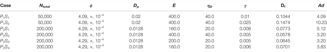
TABLE 1. Summary of parameters for all simulations, all parameters are normalized.
The computational domain is a periodic box of size 8 × 8 × 8, and 16 elements of uniform size were used in each direction. A polynomial order PN = 8 was used within each element, which yields a total resolution of around 2.1 million grid points. The third order Adams–Bashforth method was used for time integration. A fixed time step was chosen in all simulations, which ensures the maximum Courant–Friedrichs–Lewy (CFL) number to remain around 0.2. The “3/2” rule was used for de-aliasing. The PNPN-2 algorithm was applied (Maday et al., 1990; Fischer, 1997), in which pressure is solved on a coarser grid with polynomial order 6.
The DNS Model has been validated with previous DNS study by Rosales and Meneveau (2005) using the time-averaged energy spectrum. Due to the small Reynolds number used in both studies, there is no clear “−5/3” slope. The red solid curve represents the averaged non-dimensional energy spectra over cases with different Reynolds numbers. Our model results agree with the previous DNS study reasonably well (Figure 1). The forcing coefficient (α = 0.033) and the viscosity (ν = 5 × 10⁻³) are kept the same for all cases. This gives the Reynolds number of 200 based on unit characteristic velocity and length scales, and Taylor Reynolds number (Reλ) of 32. For homogeneous isotropic turbulent flow, there are no intrinsic characteristic scales for the mean flow. The Taylor Reynolds number is commonly used in homogeneous isotropic turbulence because it uses the fundamental length scale and velocity scale of turbulence to define the Reynolds number. To relate the idealized simulation conducted in this study with field condition, the Taylor Reynolds number can be used to obtain the turbulent shear rate when characteristic scales in dimensional form are given. The average Kolmogorov length scale is η = 0.049 and the average turbulent kinetic energy is kt = 0.12.

FIGURE 1. Model validation with DNS simulation results from Rosales and Meneveau (2005).
To make results relevant to geophysical or engineering applications, simulation results can be interpreted in the dimensional forms with given characteristic length scale and velocity scale. Due to the limitation of computational resources, the present study focuses on energetic environment with high turbulent shear only. For a characteristic length scale of L = 10–3 m, the characteristic velocity scale is U = 0.2 m/s, based on the Reynolds number, and the particle diameter is Dp = 12.8 μm for cases P2. The particles can be interpreted as the smallest clay-based aggregates, namely, flocculi. Flocculi seldom break down to the lowest-level primary particles even at the high turbulent shear and hence are the building blocks of large flocs. The turbulent shear rate based on the characteristic scales is 350 s−1 for all cases. The shear rate is higher than the values in most laboratory experiments and field observations; however, the model captures how turbulence affects flocculation dynamics. The Young’s modulus for soft clay is in the range of 0.5 to 5MPa, and the Poisson ratio of clay is 0.3. The Young’s modulus used in the simulation is between 6.4 and 16 kPa, which is reduced by two order of magnitude to accelerate the computation. In the JKR theory, the pull-off force to separate two particles is 3πγJKRDp/2, which can be used to define the yield strength of the floc. The softness of particles does not affect the yield-strength of flocs directly and hence the aggregation of particles. Detailed measurement on the surface energy density γ is still lacking. In this study, the surface energy density used in the JKR model is in the range of 2 × 10⁻⁴ to 1 × 10⁻³ J/m2. The stickiness of the particle can be characterized by the adhesive number, which is defined as the ratio of the yield strength of flocs represented by the surface energy density γ to the turbulent kinetic energy Ad = γ/ρktD. Because the turbulent intensity remains the same in all cases, the average floc size increases with the adhesive number as expected when the primary particle is kept the same (Table 1). In addition, the averaged floc size is almost three times greater than the Kolmogorov length scale for the cases with the largest adhesive number. However, for cases with relatively small adhesive number (case P2S2 and P2S3), the floc size is limited by the Kolmogorov length scale, and the average floc size is comparable to the Kolmogorov length scale.
The flow velocity field from case P1S1 is shown in Figure 2A. The horizontal x − y plane is located at z0 = 0. Only particles whose centers are located between z0 − Dp/2 and z0 + Dp/2 are projected to the x − y plane. The zoom in view is shown in Figure 2B to show the detailed structures of the flocs. Clusters of primary particles can be observed as flocs form. The Stokes numbers
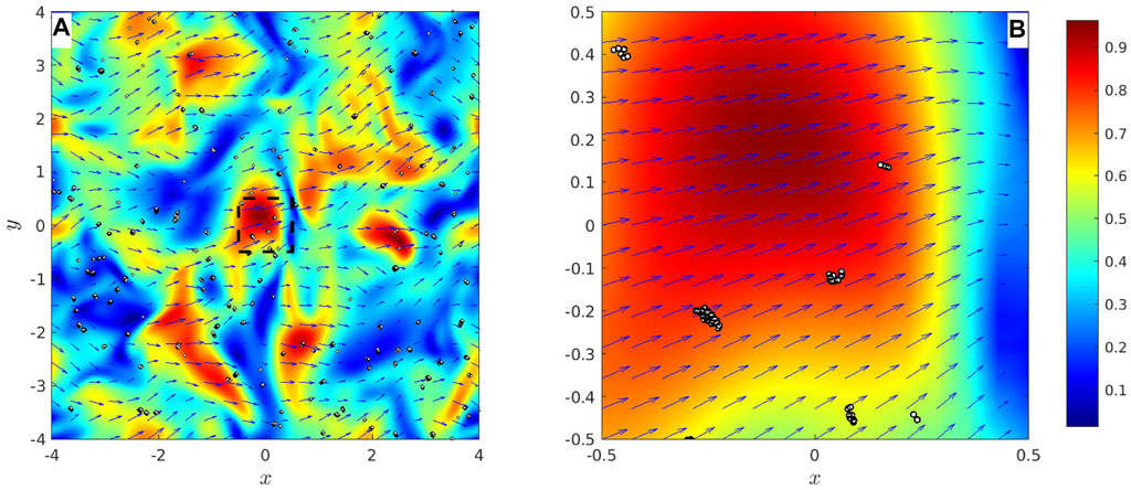
FIGURE 2. Model results. (A) Horizontal (x–y) plane of the flow field with particles from case P1S1 with relatively larger primary particles. The streamwise velocity component is used as background color. (B) Zoom in view of the velocity field and particles [black box in panel (A)].
All simulations are initialized with mono-dispersed spherical particles, which are uniformly distributed in the simulation domain. Initially, the particle velocity is set to zero. Due to collisions driven by turbulence, flocs start to form gradually and the floc size distribution evolves into an equilibrium distribution. In total, two contrasting cases, P2S1 (softer and more sticky primary particles) and P2S2 (more stiff and less sticky primary particles), are selected to investigate the dynamics. Figure 3 shows the time-evolution of the floc population
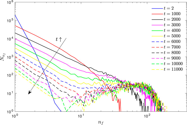
FIGURE 3. Time evolution of the floc population
FIGURE 4. Time evolution of the floc population
To further investigate the aggregation process of flocs, the time-evolution of the floc population for given floc sizes are shown in Figures 5, 6. For case P2S1, small flocs of size nf between 2 and 5 show a similar pattern (Figure 5A). The population
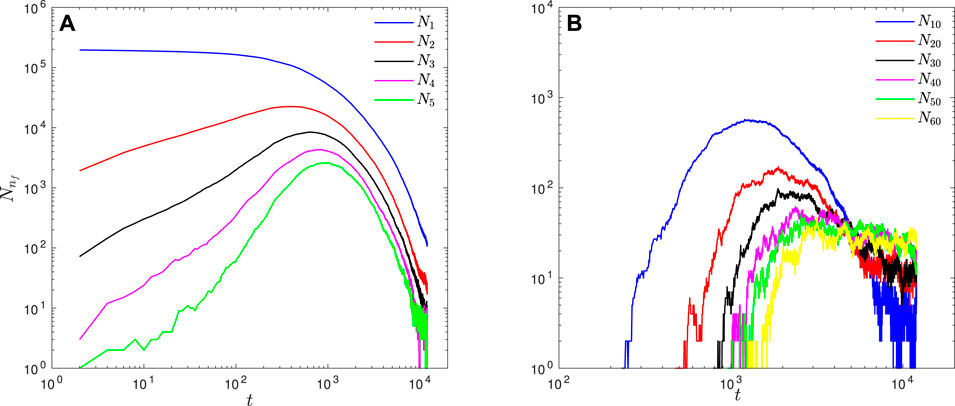
FIGURE 5. Time evolution of floc population

FIGURE 6. Time evolution of floc population
The time evolution of floc population
To better understand how physicochemical properties of the primary particle (i.e, stickiness) affect the equilibrium floc size distribution, we examine the flocculation dynamics using the population balance equation as follows:
where n (v, x, t) is the number density of flocs with volume (or size) v at time t and location x, Ws is the floc settling velocity, ui is the fluid velocity component in the i-th direction, and κ is the sum of the molecular and turbulent diffusivity. On the right hand side of the equation, Q is the aggregation kernel and Γ is the breakup kernel. β is the fragmentation distribution, which describes the created number of daughter flocs of volume v after the breakage of a mother floc of volume v′. The aggregation kernel (Q) is a function of the collision frequency and collision efficiency. The collision frequency is a function of the turbulent shear rate and increases with the turbulent shear rate. The collision efficiency is defined as the rate of successful collisions resulting in the aggregation of flocs to the total number of collisions, which is a function of the properties of sediment particles.
The first term (term I) on the right hand side represents the formation of a floc of volume v by the aggregation of two smaller flocs of volume v − v′ and v′. The second term (term II) on the right hand side represents the formation of a floc of volume v from the breakup of a larger floc of volume v′. In both term I and term II, a new floc of volume v is generated, and hence they are the construction terms. The third term (term III) represents the aggregation of a floc of volume v with another floc of volume v′ to form a larger floc of volume v + v′. The last term (term IV) represents the breakup of a floc of volume v. In both term III and term IV, a floc of volume v is consumed, and hence they are the destruction terms.
In Eq. 21, both aggregation and breakup processes in the population balance equation require parameterization, including the aggregation kernel, the breakup kernel, and the fragmentation distribution (Jeldres et al., 2015). By modeling the sediment phase as the dispersed phase using the Lagrangian framework, we can track the time-evolution of individual flocs of different size nf (or volume v = nfVp, with Vp as the volume of the primary particle) to understand the aggregate and breakup processes at the particle scale. By comparing simulation results at two consecutive time instances, aggregation and breakup of flocs can be obtained in the time-driven Lagrangian model. Considering all the flocs of size nf = 16, we investigate the state of each one of them at a time interval Δt = 2 before. Most of the flocs of size nf = 16 have remained the same over this small time interval. Some flocs would have been of a smaller size (i.e., nf < 16) at the previous time (t − Δt) and have grown to flocs of nf = 16 due to aggregation, while some of the flocs would have been larger at the previous time and have reduced in size to nf = 16 due to breakup. We refer to the previous time floc size at t − Δt as the “prior-size”. Figure 7A shows the probability density function (PDF) of the prior-size of flocs whose current size is nf = 16. Most of the flocs of prior-size nf = 16 that have remained the same without aggregation or breakup and are not included in the analysis. In Figure 7A, the blue circle symbols represent the source of nf = 16 flocs. The circles to the left of the dash line correspond to the PDF of smaller flocs aggregating and becoming nf = 16 floc, while circles to the right of the dash line correspond to the PDF of larger flocs breaking up and generating a daughter floc of size nf=16. These are terms I and II on the right hand side of (21).

FIGURE 7. Case P2S1 with the largest stickiness. (A) Probability density function (PDF) that a floc of size nf becomes a floc of size nf = 16 in a non-dimensional time period of 2 (blue circles) and the PDF that a floc of size nf = 16 evolves into a floc of size nf over the same period (red pluses). (B,C) Same as frame-(A) for nf = 32 and 64.
In a similar manner, the red plus symbols represent the sink of nf = 16 flocs, i.e., they measure the PDF of what a floc of size nf = 16 floc becomes after a small time interval of Δt = 2. The pluses to the left of the dash line correspond to the PDF of smaller flocs that form from the breakup of nf = 16 flocs, while pluses to the right of the dash line correspond to the PDF of larger flocs that are formed by the aggregation of a floc of size nf = 16 with another floc (or other flocs). These are terms III and IV on the right hand side of (Eq. 21). The collapse of the two curves (circle sources and plus sinks) suggests a dynamic equilibrium with the balance between the aggregation and breakup processes. The PDF is almost uniform for small flocs. A peak is evident at nf ≈ 80. A power–law distribution of the PDF can be observed for the large flocs with nf > 80. For small flocs, we observe a drastic drop from the peak to nf ≈ 30, and the distribution is quite uniform for nf ≤ 30.
We carried out the same analysis for flocs of size nf = 32 (Figure 7B), the power–law distribution is evident for large flocs of nf > 80. A uniform distribution can be observed between nf = 32 and 80. For smaller flocs of nf < 32, the distribution shows a minimum around nf ≈ 9 and peaks around nf = 32 and nf = 1 (primary particles). For floc of size nf = 64 (Figure 7C), the power–law distribution is still evident for large flocs of nf > 80. In addition, a significant change of the slope for large flocs of size greater than nf = 150 can be identified. For small flocs of nf < 64, the distribution shows a uniform distribution between 20 and 60 and two peaks near nf = 64 and nf = 1 (primary particles). For case P2S2 with less sticky and more stiff primary particles, the terms are plotted for flocs of size nf = 8, 16, and 24 (Figure 8). The PDFs for flocs of different size are quite similar. It shows a power–law relation for large flocs of nf ≥ 16. For smaller flocs of nf < 16, the distribution exhibits a minimum at nf = 5 and two peaks at nf = 16 and nf = 1 (primary particle). Compared to the case P2S1 with the stickies primary particles, the presence of the uniform distribution for intermediate-sized flocs (nf between 30 and 50 in case P2S1) is not evident in case P2S2.
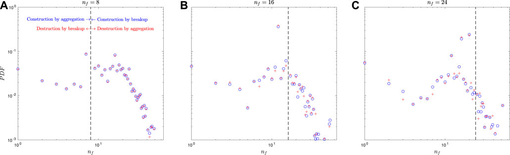
FIGURE 8. Case P2S2 with smaller stickiness and larger stiffness. (A) Probability density function (PDF) that a floc of size nf becomes a floc of size nf = 8 in a non-dimensional time period of 2 (blue circles) and the PDF that a floc of size nf = 8 evolves into a floc of size nf over the same period (red pluses). (B,C) Same as frame-(A) for nf = 16 and 24.
In both cases, at the equilibrium stage when the breakup and aggregation processes balance with each other, simulation results show that the construction by aggregation is primarily balanced by the destruction by breakup and the construction by breakup is primarily balanced by the destruction by aggregation. At the microscopic level, each aggregation or breakup pathway is reversible and hence in a dynamic equilibrium. With given aggregation and breakup kernels, equilibrium solutions of the floc size distribution exist (Vigil, 2009), and the mathematical form of the equilibrium floc size distribution could be derived.
An equilibrium floc size distribution develops when the aggregation process balances with the breakup process. The floc size distribution is modeled as a function of nf, instead of the floc size Df, because the number density (n) in Equation (21) is expressed as a function of the floc volume v. In this study, flocs are consisted of slightly overlapping identical spheres, and the volume of a floc consisted of nf primary particles can be approximated by nf as
where ln nf follows the normal distribution, μ is the mean, and σ2 is the variance.
The Weibull distribution is a special form of Gamma distribution with two parameters, namely, the scaling parameter λ and the shape parameter k.
The Weibull distribution interpolates between the exponential distribution and Rayleigh distribution. The shape parameter k affects the shape of the distribution rather than simply shifting or stretching it. Figure 9 shows the curve fitting for case P2S1 (panel a), P2S2 (panel b), and P2S3 (panel c). For case P2S1 with the stickiest primary particles, model results fit better with the Weibull distribution, while results from case P2S2 with less sticky but more stiff primary particles fit better with the lognormal distribution. For case P2S3, neither lognormal nor Weibull distribution can fit the data for the entire range of the floc size nf. To assess the performance of different distributions, the Anderson–Darling (AD) test (Anderson and Darling, 1952) was conducted, which is based on the empirical cumulative distribution obtained from the sample. The AD test is commonly used to test if a sample of data comes from a population with a specific distribution. We used the significant level of α = 0.01, which is commonly used in statistical hypothesis test (Fisher, 1992). The results are summarized in Table 2, where Es is the sum of squared residual errors. The accepted hypothesis for each case is shown with “*” in Table 2, which means the optimal descriptor for the floc size distribution. For the case with less sticky primary particles (case P2S2), the lognormal distribution fits better and for the cases with very sticky primary particles (case P1S2 and P2S1), the Weibull distribution fits better. The AD test rejects both lognormal and Weibull distribution hypothesis for most cases, suggesting neither lognormal nor Weibull distribution can accurately predict the floc size distribution. For instance, the lognormal distribution fits better for small flocs and also captures the peak more accurately in case P2S3 (Figure 9C), while the Weibull distribution fits better for large flocs (nf > 35). The adjusted coefficient of determination
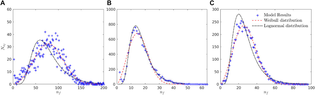
FIGURE 9. Floc size distribution represented by
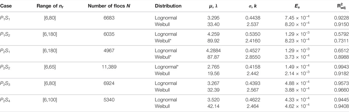
TABLE 2. Anderson–Darling test results and the adjusted coefficient of determination
Floc size distribution from P2S1 fits better with the Weibull distribution. To further investigate the floc size distribution from case P2S1, we plotted model results under log-log scale (Figure 10A) and semi-log scale (Figure 10B). We averaged
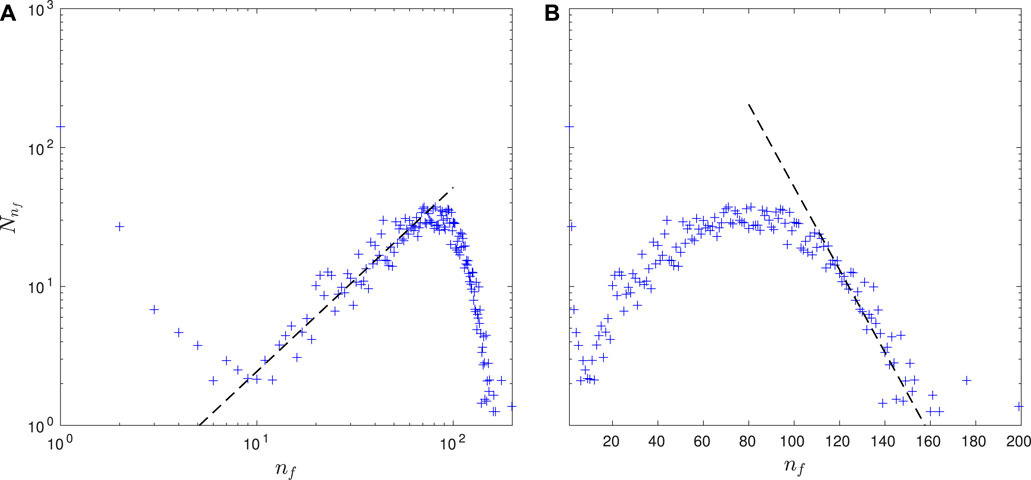
FIGURE 10. Floc size distribution from case P2S1 (A) power-law fit and (B) exponential fit.
Different mathematical formulas of floc size distribution arise in the aggregation or breakage processes (Huber et al., 2006). Lognormal distribution has been observed in particle growth or coagulation processes (Smoluchowski, 1918; Friedlander and Wang, 1966), in which aggregation process dominates the dynamics. On the other hand, Weibull distribution has been commonly observed in the fragmentation process of large particles (Brown and Wohletz, 1995). In the flocculation process, both the aggregation and fragmentation processes play an important role. At the equilibrium state, a floc can be constructed either by aggregation of smaller flocs or breakup from larger flocs. To further understand under which circumstances a lognormal or Weibull distribution performs better, we analyzed the dominant floc construction mechanisms at the equilibrium stage. Figure 11 shows the relative importance of construction by aggregation and construction by the breakup for flocs of size nf from the two contrasting cases P2S1 and P2S2. In case P2S1 (Figure 11A), the majority of small flocs are constructed by breakup of larger flocs, while large flocs (nf > 75) are mainly constructed by aggregation as expected. The aggregation and breakup processes play equally important roles for flocs in the range of 30<nf < 75. The primary particles first aggregate into microflocs, the microflocs are quite resilient to turbulent shear and serve as the building blocks for larger flocs. For case P2S2 (Figure 11B), we observe a monotonic increase in relative importance for aggregation and a decrease for breakup process with respect to nf. In general, a large portion of flocs (nf < 75) in case P2S1 are generated mainly from breakup of larger flocs. However, in case P2S2, breakup only controls the formation of a small portion of flocs with nf < 15, and the aggregation process dominates the formation of flocs for a wide range of flocs. The lognormal distribution (case P2S2) develops when the large flocs grow gradually from primary particles without the intermediate stage (the formation of “microflocs”). This behavior has not been observed in laboratory experiments before, and future laboratory studies are required to test whether this is an artifact of the numerical model or an actual physical process.
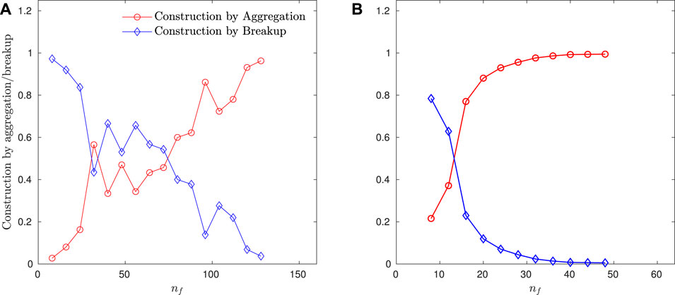
FIGURE 11. Relative importance of the two construction mechanisms for flocs of size n. (A) Case P2S1 and (B) P2S2.
Mathematical approach of floc modeling that has gained much interest by modelers is the fractal representation of flocs (Kranenburg, 1994; Merckelbach, 2000; Graham and Manning, 2007). Fractal theory is dependent on the successive aggregations of self-similar flocs, thereby producing a structure that is independent of the scale (or scale invariant). This is similar to the order-of-aggregation theory (Krone, 1963). Following the fractal theory, simple power laws can be used to describe floc properties such as floc density and settling velocity, as well as the aggregation and breakup processes (Winterwerp, 1998). Although some studies suggest that individually some natural muddy flocs (particularly those with high organic contents) may not be fully fractal in structure (Zhang et al., 2018; Spencer et al., 2021), the wider examination of in situ floc populations shows that a fractal representation of flocs still has many merits (Dyer and Manning, 1999; Winterwerp et al., 2006). The fractal dimension d0 used to characterize the floc structure is defined as
where nf is the total number of the primary particles consisting the floc, Df is the floc size and Dp is the primary particle diameter. The major axis length (longest axis) is used as floc size Df, which is obtained by the principal component analysis (PCA). In general, the fractal dimension (d0) is 1 for chain-like flocs and 2 for flat plane-like flocs. Flocs with fractal dimension close to 3 have compact structure and spherical shape.
Flocs with the same number of primary particles (nf) can exhibit different structures, and the averaged fractal dimension
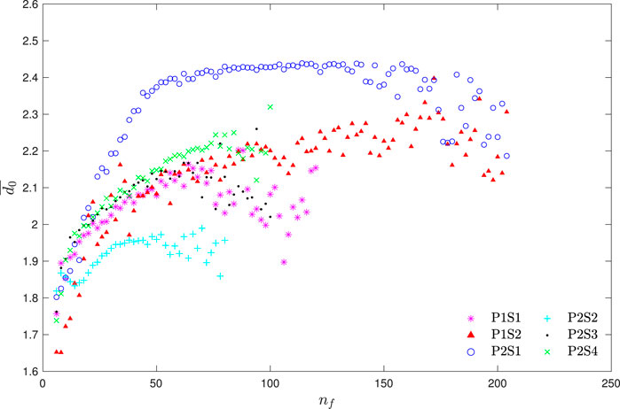
FIGURE 12. Averaged fractal dimension
In contrast, in case P2S2 with the least sticky primary particles, the fractal dimension increases to the peak value around 1.95 and then drops for large flocs. The decrease in the fractal dimension for large flocs has also been observed by Khelifa and Hill (2006) and Maggi (2007). Our numerical results suggest the scale-dependence of floc structure as the fractal dimension is not constant for the entire range of the floc size. A variable fractal dimension should be considered to characterize the flocs.
In general, for the cases with the same primary particle diameter, primary particles with small adhesive numbers (or surface energy density) lead to flocs with smaller fractal dimensions, and primary particles with large adhesive numbers generate more compact flocs with fractal dimension as large as 2.4 in case P2S1. Floc compaction by the breakage-regrowth and restructuring mechanisms are more pronounced in the case with the stickiest primary particle. By comparing case P2S2 and P2S3, the stiffness of the particle also affects the floc structures. Primary particles with larger Young’s modulus (case P2S2) lead to flocs with smaller fractal dimension.
A two-phase Eulerian–Lagrangian framework was implemented to investigate the equilibrium floc size distribution of cohesive sediment in homogeneous isotropic turbulence. The primary particles are modeled as identical sticky soft spheres, and particle–particle interactions are modeled by the discrete element method. The adhesive contact JKR model was implemented to model cohesive sediment particles, which is a tensile force model with hysteretic effect. In the adhesive contact model, the pull-off force to break two particles apart scales with both the particle size and the surface energy density (i.e., the physicochemical properties of the primary particle).
A series of numerical simulations were conducted by varying the size and properties of the primary particles. At the equilibrium state, the construction by breakup is balanced with the destruction by aggregation, and the construction by aggregation is balanced with the destruction by breakup. The equilibrium floc size distribution depends on primary particle properties, including the stiffness and the surface energy density. For cases with more sticky primary particles, the floc size distribution can be better described by the Weibull distribution with a shape parameter around 2.5. In addition, at the intermediate stage, a staircase structure develops in the floc size distribution. The primary particles first form the ‘microflocs’, which serve as the building blocks for large flocs. For the case with less sticky primary particles, the lognormal distribution performs better. Flocs grow gradually from primary particles without the intermediate stage of ‘microflocs’.
By analyzing the construction mechanisms of flocs of different size, when the Weibull distribution develops, construction by breakup and construction by aggregation are of equal importance for the intermediate-sized flocs. The fractal dimension of large flocs then decreases with floc size, suggesting large “macroflocs” are more porous and fragile. For less sticky particles, the lognormal distribution develops, and the aggregation dominates the floc construction for a wide range of flocs. The fractal dimension of flocs first increases with floc size, reaches the peak value, and then decreases with the floc size. However, given the similarity between the lognormal and Weibull distributions and hence the difficulties in distinguishing between them in confidence, it is recommended to choose the floc size distribution and make interpretations in practice with caution.
Due to the limited computational resources, the current simulation focuses on the high-energy environments with large turbulent shear rate (350 s−1 in this study). Simulations with more particles (several millions to billions of particles) are therefore required for more realistic cohesive sediment transport studies in low-to moderate-energy environments. In addition, current model framework oversimplifies the hydrodynamic interactions among particles without the influence from neighboring particles. For cohesive sediment, the particle Reynolds number based on Stokes settling velocity is small, and hence the sheltering and blockage effects from neighboring particles could play an important role. The sheltering effects from neighboring particles lead to reduced hydrodynamic drag, and hence could affect the breakup processes. A more sophisticated efficient model that can accurately predict hydrodynamic interactions among a large amount of particles is required and will be the future work.
The datasets presented in this study can be found in online repositories. The names of the repository/repositories and accession number(s) can be found at: https://figshare.com/articles/dataset/FlocSizeDistribution/16619734.
MY: methodology; formal analysis; and writing—original draft, review, and editing. XY: supervision; conceptualization; methodology; formal analysis; writing—original draft, review, and editing. SB: conceptualization; methodology, and writing—review and editing. AM: writing–review and editing.
This work is funded by the United States Army Engineering Research and Development Center under the Cooperative Ecosystem Studies Unit (CESU) grant W912HZ-21-2-0035. AM’s contribution toward this research was also partly supported by the United States National Science Foundation under grants OCE-1736668 and OCE-1924532, TKI-MUSA project 11204950-000-ZKS-0002, and HR Wallingford company research FineScale project (ACK3013-62).
Author AM was employed by the company HR Wallingford.
The remaining authors declare that the research was conducted in the absence of any commercial or financial relationships that could be construed as a potential conflict of interest.
All claims expressed in this article are solely those of the authors and do not necessarily represent those of their affiliated organizations, or those of the publisher, the editors, and the reviewers. Any product that may be evaluated in this article, or claim that may be made by its manufacturer, is not guaranteed or endorsed by the publisher.
All simulations were carried out on the HiperGator super computer at the University of Florida. Computer resources, technical expertise, and assistance provided by the HiperGator are gratefully acknowledged. The CFD model nek5000 is developed primarily by the Argonne National Laboratory at https://nek5000.mcs.anl.gov/, and the DEM model LAMMPS is developed by Sandia National Laboratories at https://lammps.sandia.gov/.
Akiki, G., Moore, W. C., and Balachandar, S. (2017). Pairwise-interaction Extended Point-Particle Model for Particle-Laden Flows. J. Comput. Phys. 351, 329–357. doi:10.1016/j.jcp.2017.07.056
Anderson, T. W., and Darling, D. A. (1952). Asymptotic Theory of Certain “Goodness of Fit” Criteria Based on Stochastic Processes. Ann. Math. Stat. 23, 193–212. doi:10.1214/aoms/1177729437
Balachandar, S., and Eaton, J. K. (2010). Turbulent Dispersed Multiphase Flow. Annu. Rev. Fluid Mech. 42, 111–133. doi:10.1146/annurev.fluid.010908.165243
Baugh, J. V., and Manning, A. J. (2007). An Assessment of a New Settling Velocity Parameterisation for Cohesive Sediment Transport Modeling. Cont. Shelf Res. 27 (13), 1835–1855. doi:10.1016/j.csr.2007.03.003
Brown, W. K., and Wohletz, K. H. (1995). Derivation of the Weibull Distribution Based on Physical Principles and its Connection to the Rosin-Rammler and Lognormal Distributions. J. Appl. Phys. 78 (4), 2758–2763. doi:10.1063/1.360073
Byun, J., and Son, M. (2020). On the Relationship between Turbulent Motion and Bimodal Size Distribution of Suspended Flocs. Estuar. Coast. Shelf Sci. 245, 106938. doi:10.1016/j.ecss.2020.106938
Dyer, K. R., and Manning, A. J. (1999). Observation of the Size, Settling Velocity and Effective Density of Flocs, and Their Fractal Dimensions. J. Sea Res. 41 (1-2), 87–95. doi:10.1016/s1385-1101(98)00036-7
Dyer, K. R. (1989). Sediment Processes in Estuaries: Future Research Requirements. J. Geophys. Res. 94 (C10), 14327–14339. doi:10.1029/jc094ic10p14327
Edmonds, D. A., and Slingerland, R. L. (2010). Significant Effect of Sediment Cohesion on Delta Morphology. Nat. Geosci. 3, 105–109. doi:10.1038/ngeo730
Eisma, D. (1986). Flocculation and De-flocculation of Suspended Matter in Estuaries. Neth. J. Sea Res. 20 (2-3), 183–199. doi:10.1016/0077-7579(86)90041-4
Fang, Z., Patterson, B. R., and Turner, M. E. (1993). Modeling Particle Size Distributions by the Weibull Distribution Function. Mater. Charact. 31 (3), 177–182. doi:10.1016/1044-5803(93)90058-4
Fischer, P. F. (1997). An Overlapping Schwarz Method for Spectral Element Solution of the Incompressible Navier-Stokes Equations. J. Comput. Phys. 133 (1), 84–101. doi:10.1006/jcph.1997.5651
Fischer, P. F., Lottes, J. W., and Kerkemeier, S. G. (2008). Nek5000. Available at: http://nek5000.mcs.anl.gov.
Fisher, R. A. (1992). “Statistical Methods for Research Workers,” in Breakthroughs in Statistics (New York, NY: Springer), 66–70. doi:10.1007/978-1-4612-4380-9_6
Friedlander, S. K., and Wang, C. S. (1966). The Self-Preserving Particle Size Distribution for Coagulation by Brownian Motion. J. Colloid interface Sci. 22 (2), 126–132. doi:10.1016/0021-9797(66)90073-7
Geyer, W. R., Hill, P., Milligan, T., and Traykovski, P. (2000). The Structure of the Eel River Plume during Floods. Cont. Shelf Res. 20 (16), 2067–2093. doi:10.1016/s0278-4343(00)00063-7
Graham, G. W., and Manning, A. J. (2007). Floc Size and Settling Velocity within a Spartina Anglica Canopy. Cont. Shelf Res. 27 (8), 1060–1079. doi:10.1016/j.csr.2005.11.017
Hayter, E. J., and Mehta, A. J. (1986). Modelling Cohesive Sediment Transport in Estuarial Waters. Appl. Math. Model. 10 (4), 294–303. doi:10.1016/0307-904x(86)90061-2
Hill, P. S. (1996). Sectional and Discrete Representations of Floc Breakage in Agitated Suspensions. Deep Sea Res. Part I Oceanogr. Res. Pap. 43 (5), 679–702. doi:10.1016/0967-0637(96)00030-1
Hosoda, K., Matsuura, T., Suzuki, H., and Yomo, T. (2011). Origin of Lognormal-like Distributions with a Common Width in a Growth and Division Process. Phys. Rev. E Stat. Nonlin Soft Matter Phys. 83, 031118. doi:10.1103/PhysRevE.83.031118
Huber, P., Roux, E., Mauret, J. C., and Carre, B. (2006). Characterising the Floc Size Distribution of Flowing Pulp Suspensions: from Fibre Flocculation to Sheet Formation. Appita Technol. Innov. Manuf. Environ. 59, 37. doi:10.3316/informit.586267214881170
Hunt, J. R. (1982). Self-similar Particle-Size Distributions during Coagulation: Theory and Experimental Verification. J. Fluid Mech. 122, 169–185. doi:10.1017/s0022112082002158
Jeldres, R. I., Concha, F., and Toledo, P. G. (2015). Population Balance Modelling of Particle Flocculation with Attention to Aggregate Restructuring and Permeability. Adv. colloid interface Sci. 224, 62–71. doi:10.1016/j.cis.2015.07.009
Khelifa, Ali, and Hill, Paul S. (2006). Models for Effective Density and Settling Velocity of Flocs. J. Hydraulic Res. 44 (3), 390–401. doi:10.1080/00221686.2006.9521690
Kiss, L. B., Söderlund, J., Niklasson, G. A., and Granqvist, C. G. (1999). New Approach to the Origin of Lognormal Size Distributions of Nanoparticles. Nanotechnology 10 (1), 25–28. doi:10.1088/0957-4484/10/1/006
Kolmogorov, A. N. (1941b). Dissipation of Energy in Locally Iscotropic Turbulence. Proc. USSR Acad. Sci. 32, 16.
Kolmogorov, A. N. (1941a). The Local Structure of Turbulence in Incompressible Viscous Fluid for Very Large Reynolds Numbers. Proc. USSR Acad. Sci. 30, 301.
Kondolf, G. M., and Adhikari, A. (2000). Weibull vs. Lognormal Distributions for Fluvial Gravels. J. Sediment. Res. 70 (3), 456–460. doi:10.1306/2dc4091e-0e47-11d7-8643000102c1865d
Kranenburg, C. (1994). The Fractal Structure of Cohesive Sediment Aggregates. Estuar. Coast. Shelf Sci. 39 (5), 451–460. doi:10.1006/ecss.1994.1075
Krone, R. B. (1963). A Study of Rheological Properties of Estuarial Sediments. Report No. 63-68. Berkeley: Hydraulic Engineering Laboratory and Sanitary Engineering Research Laboratory, University of California.
Li, D., and Ganczarczyk, J. (1991). Size Distribution of Activated Sludge Flocs. Res. J. water Pollut. control Fed. 63 (5), 806–814
Luding, S. (2008). Cohesive, Frictional Powders: Contact Models for Tension. Granul. matter 10 (4), 235–246. doi:10.1007/s10035-008-0099-x
Lundgren, T. S. (2003). Linearly Forces Isotropic Turbulence. Minnesota Univ Minneapolis. Ph.D. thesis.
Maday, Y., Patera, A. T., and Rnquist, E. M. (1990). An Operator-Integration-Factor Splitting Method for Time-dependent Problems: Application to Incompressible Fluid Flow. J. Sci. Comput. 5, 263–292. doi:10.1007/bf01063118
Maggi, F. (2007). Variable Fractal Dimension: A Major Control for Floc Structure and Flocculation Kinematics of Suspended Cohesive Sediment. J. Geophys. Res. Oceans 112 (C7), 3951. doi:10.1029/2006jc003951
Manning, A. J. (2001). A Study of the Effects of Turbulence on the Properties of Flocculated Mud. Ph.D. Thesis. Institute of Marine Studies, University of Plymouth.
Manning, A. J., Bass, S. J., and Dyer, K. R. (2006). Floc Properties in the Turbidity Maximum of a Mesotidal Estuary during Neap and Spring Tidal Conditions. Mar. Geol. 235 (1-2), 193–211. doi:10.1016/j.margeo.2006.10.014
Manning, A. J., and Dyer, K. R. (1999). A Laboratory Examination of Floc Characteristics with Regard to Turbulent Shearing. Mar. Geol. 160 (1-2), 147–170. doi:10.1016/s0025-3227(99)00013-4
Manning, A. J., and Schoellhamer, D. H. (2013). Factors Controlling Floc Settling Velocity along a Longitudinal Estuarine Transect. Mar. Geol. 345, 266–280. doi:10.1016/j.margeo.2013.06.018
Manning, A. J. (2004). The Observed Effects of Turbulence on Estuarine Flocculation. J. Coast. Res. 41, 90–104
Marshall, J. S. (2009). Discrete-element Modeling of Particulate Aerosol Flows. J. Comput. Phys. 228 (5), 1541–1561. doi:10.1016/j.jcp.2008.10.035
McAnally, W. H., and Mehta, A. J. (2001). Collisional Aggregation of Fine Estuarine Sediments. Coast. Estuar. Fine Sediment Process. - Proc. Mar. Sci. 3, 19
Mehta, A. J., and Lott, J. W. (1987). Sorting of Fine Sediment during Deposition. Proc. Conf. Adv. Underst. Coast. Sediment Process. 1, 348
Mehta, A. J., Manning, A. J., and Khare, Y. P. (2014). A Note on the Krone Deposition Equation and Significance of Floc Aggregation. Mar. Geol. 354, 34–39. doi:10.1016/j.margeo.2014.04.002
Mindlin, R. D. (1949). Compliance of Elastic Bodies in Contact. J. Appl. Mech. ASME 16 (3), 259–268. doi:10.1115/1.4009973
Mouri, H., Hori, A., and Takaoka, M. (2009). Large-scale Lognormal Fluctuations in Turbulence Velocity Fields. Phys. fluids 21, 7936. doi:10.1063/1.3147936
Plimpton, S. (1995). Fast Parallel Algorithms for Short-Range Molecular Dynamics. J. Comput. Phys. 117 (1), 1–19. doi:10.1006/jcph.1995.1039
Prandle, D., Lane, A., and Manning, A. J. (2005). Estuaries Are Not So Unique. Geophys. Res. Lett. 32 (23), 24797. doi:10.1029/2005gl024797
Pushkin, D. O., and Aref, H. (2002). Self-similarity Theory of Stationary Coagulation. Phys. fluids 14, 694–703. doi:10.1063/1.1430440
Rosales, C., and Meneveau, C. (2005). Linear Forcing in Numerical Simulations of Isotropic Turbulence: Physical Space Implementations and Convergence Properties. Phys. fluids 17 (9), 095106. doi:10.1063/1.2047568
Saha, D., Babler, M. U., Holzner, M., Soos, M., Lüthi, B., Liberzon, A., et al. (2016). Breakup of Finite-Size Colloidal Aggregates in Turbulent Flow Investigated by Three-Dimensional (3d) Particle Tracking Velocimetry. Langmuir 32 (1), 55–65. doi:10.1021/acs.langmuir.5b03804
Sheremet, A., Sahin, C., and Manning, A. J. (2017). Flocculation: A General Aggregation-Fragmentation Framework. Int. Conf. Coast. Eng. 35, 27. doi:10.9753/icce.v35.sediment.27
Smoluchowski, M. v. (1918). Versuch einer mathematischen Theorie der Koagulationskinetik kolloider Lösungen. Z. für Phys. Chem. 92U (1), 129–168. doi:10.1515/zpch-1918-9209
Soulsby, R. L., Manning, A. J., Spearman, J., and Whitehouse, R. J. S. (2013). Settling Velocity and Mass Settling Flux of Flocculated Estuarine Sediments. Mar. Geol. 339, 1–12. doi:10.1016/j.margeo.2013.04.006
Spencer, K. L., Wheatland, J. A. T., Bushby, A. J., Carr, S. J., Droppo, I. G., and Manning, A. J. (2021). A Structure-Function Based Approach to Floc Hierarchy and Evidence for the Non-fractal Nature of Natural Sediment Flocs. Sci. Rep. 11, 14012. doi:10.1038/s41598-021-93302-9
Spicer, P. T., and Pratsinis, S. E. (1996). Coagulation and Fragmentation: Universal Steady-State Particle-Size Distribution. AIChE J. 42 (6), 1612–1620. doi:10.1002/aic.690420612
Sun, R., Xiao, H., and Sun, H. (2018). Investigating the Settling Dynamics of Cohesive Silt Particles with Particle-Resolving Simulations. Adv. Water Resour. 111, 406–422. doi:10.1016/j.advwatres.2017.11.012
Sundaram, S., and Collins, L. R. (1997). Collision Statistics in an Isotropic Particle-Laden Turbulent Suspension. Part 1. Direct Numerical Simulations. J. Fluid Mech. 335, 75–109. doi:10.1017/s0022112096004454
Tambo, N., and Watanabe, Y. (1984). Physical Aspect of Flocculation Process-III. Water Res. 18 (4), 695–707. doi:10.1016/0043-1354(84)90165-9
Tolhurst, T. J., Gust, G., and Paterson, D. M. (2002). The Influence of an Extracellular Polymeric Substance (EPS) on Cohesive Sediment Stability. Proc. Mar. Sci. 5, 409–425. doi:10.1016/s1568-2692(02)80030-4
Tsuji, Y., Kawaguchi, T., and Tanaka, T. (1993). Discrete Particle Simulation of Two-Dimensional Fluidized Bed. Powder Technol. 77 (1), 79–87. doi:10.1016/0032-5910(93)85010-7
van Leussen, W. (1994). Estuarine Macroflocs and Their Role in Fine-Grained Sediment Transport. Ph.D. Thesis. The Netherlands: University of Utrecht.
van Leussen, W. (1997). “The Kolmogorov Microscale as a Limiting Value for the Floc Sizes of Suspended Fine-Grained Sediments in Estuaries,” in Cohesive Sediments (New York: Wiley), 45–62
Vigil, R. D. (2009). On Equilibrium Solutions of Aggregation-Fragmentation Problems. J. colloid interface Sci. 336 (2), 642–647. doi:10.1016/j.jcis.2009.04.061
Vowinckel, B., Withers, J., Luzzatto-Fegiz, P., and Meiburg, E. (2019). Settling of Cohesive Sediment: Particle-Resolved Simulations. J. Fluid Mech. 858, 5–44. doi:10.1017/jfm.2018.757
Wang, Y., Alonso-Marroquin, F., and Guo, W. W. (2015). Rolling and Sliding in 3-D Discrete Element Models. Particuology 23, 49–55. doi:10.1016/j.partic.2015.01.006
Winterwerp, J. C. (1998). A Simple Model for Turbulence Induced Flocculation of Cohesive Sediment. J. Hydraulic Res. 36 (3), 309–326. doi:10.1080/00221689809498621
Winterwerp, J. C., Manning, A. J., Martens, C., de Mulder, T., and Vanlede, J. (2006). A Heuristic Formula for Turbulence-Induced Flocculation of Cohesive Sediment. Estuar. Coast. Shelf Sci. 68 (1-2), 195–207. doi:10.1016/j.ecss.2006.02.003
Winterwerp, J. C., Uittenbogaard, R. E., and De Kok, J. M. (2000). Rapid Siltation from Saturated Mud Suspensions. Proc. Mar. Sci. 3, 125–146. doi:10.1016/s1568-2692(00)80117-5
Winterwerp, J. C., and van Kesteren, W. G. M. (2004). Introduction to the Physics of Cohesive Sediment in the Marine Environment, Amsterdam, Netherlands: Elsevier.
Ye, L., Manning, A. J., and Hsu, T.-J. (2020). Oil-mineral Flocculation and Settling Velocity in Saline Water. Water Res. 173, 115569. doi:10.1016/j.watres.2020.115569
Yeung, P. K., Pope, S. B., Lamorgese, A. G., and Donzis, D. A. (2006). Acceleration and Dissipation Statistics of Numerically Simulated Isotropic Turbulence. Phys. Fluids 18, 065103. doi:10.1063/1.2204053
Zhang, N., Thompson, C. E. L., Townend, I. H., Rankin, K. E., Paterson, D. M., and Manning, A. J. (2018). Nondestructive 3D Imaging and Quantification of Hydrated Biofilm-Sediment Aggregates Using X-Ray Microcomputed Tomography. Environ. Sci. Technol. 52 (22), 13306–13313. doi:10.1021/acs.est.8b03997
Zhou, Z. Y., Kuang, S. B., Chu, K. W., and Yu, A. B. (2010). Discrete Particle Simulation of Particle-Fluid Flow: Model Formulations and Their Applicability. J. Fluid Mech. 661, 482–510. doi:10.1017/s002211201000306x
Keywords: cohesive sediment, floc size distribution, two phase approach, discrete element method (DEM), dynamic equilibrium
Citation: Yu M, Yu X, Balachandar S and Manning AJ (2022) Floc Size Distributions of Cohesive Sediment in Homogeneous Isotropic Turbulence. Front. Earth Sci. 10:815652. doi: 10.3389/feart.2022.815652
Received: 15 November 2021; Accepted: 21 June 2022;
Published: 19 July 2022.
Edited by:
Katrien Van Landeghem, Bangor University, United KingdomReviewed by:
Guoxiang Wu, Ocean University of China, ChinaCopyright © 2022 Yu , Yu, Balachandar and Manning . This is an open-access article distributed under the terms of the Creative Commons Attribution License (CC BY). The use, distribution or reproduction in other forums is permitted, provided the original author(s) and the copyright owner(s) are credited and that the original publication in this journal is cited, in accordance with accepted academic practice. No use, distribution or reproduction is permitted which does not comply with these terms.
*Correspondence: Xiao Yu, eGlhby55dUBlc3NpZS51ZmwuZWR1
Disclaimer: All claims expressed in this article are solely those of the authors and do not necessarily represent those of their affiliated organizations, or those of the publisher, the editors and the reviewers. Any product that may be evaluated in this article or claim that may be made by its manufacturer is not guaranteed or endorsed by the publisher.
Research integrity at Frontiers
Learn more about the work of our research integrity team to safeguard the quality of each article we publish.