 Yuan Wang
 Qingyu You
 Tianyao Hao
95% of researchers rate our articles as excellent or good
Learn more about the work of our research integrity team to safeguard the quality of each article we publish.
Find out more
ORIGINAL RESEARCH article
Front. Earth Sci. , 24 January 2022
Sec. Solid Earth Geophysics
Volume 10 - 2022 | https://doi.org/10.3389/feart.2022.812744
This article is part of the Research Topic Understanding the Marginal Seas of Northeast Asia for Tectonics and Submarine Geohazards View all 13 articles
Scholte-wave dispersion analysis is effective at imaging the relatively low shear-wave velocity of shallow marine sediments in marginal seas. The combination of a four-component ocean-bottom-seismometer (OBS) and a towed air-gun source can economically and effectively acquire the marine dispersive seismic data. Extracting higher-order dispersive Scholte wave modes is the most critical problem in the dispersion analysis method. The extremely low shear-wave velocity and severe attenuation in the top hundreds of meters of marginal sea sediment provide an uneven dispersive energy distribution for the four components of the Scholte wave data. The fundamental mode dispersive energy dominates in the vertical component and higher-order modes dominate in the horizontal component. We developed the method of the four-component OBS Scholte velocity-spectra stacking, which can effectively, rapidly, and robustly extract higher-order modes. We imaged the shear-wave velocity structure of complicated shallow marine sediment in the North Yellow Sea using an active OBS seismic profile with a large-volume air-gun array. The fourth higher-order Scholte wave mode can be imaged with the four-component velocity-spectra stacking method with a lower frequency range of 1.0–7.0 Hz. Only the second-order mode can be recognized from the dispersion energy image of the single vertical component. The joint inversion of multimode dispersion curves can provide more accuracy and deeper constraints for the inverted model; thus, the constraint depth with five modes increases by a factor of 1.9 compared with single fundamental mode inversion. The inverted profile suggests a low shear-wave velocity of 123–670 m/s and strong lateral variations within 350 m. The main regional geological structures are shown by the inverted shear-wave velocity structure.
Imaging suboceanic shear-wave velocity (
The dispersive characteristics of interfacial and surface waves are widely used to estimate the
The vertical or radial component of an interfacial wave that travels on the water-sediment interface in the marine environment is known as a Scholte wave and is analogous to Rayleigh waves on land (Scholte, 1947). Its transverse component is known as a Love wave (Love, 1911), both in this case and on land. Scholte waves can be detected through a combination of a single deployed underwater seismic station and multiple air-gun shots on the sea surface, which is known as the “stationary-receiver” method (Klein et al., 2005). An ocean-bottom seismometer (OBS) (also known as an ocean-bottom hydrophone or ocean-bottom node) is generally used as the ocean-bottom seismic station as it is cheaper and technically simpler for marine fieldwork. However, acquiring marine Love-wave data is more complex because of the need for an ocean-bottom P-SH type of source (e.g., shear-wave vibrator; Socco et al., 2011).
The single vertical component of OBS active source Scholte-wave data was used to investigate the
This study considers the possibility and potential of using the 4C OBS Scholte-wave data to image higher-order dispersive modes. Moreover, the feasibility of imaging the complex shallow marine sediment of marginal seas using the Scholte-wave dispersion inversion method is verified. We begin by presenting the acquisition and geometry of the OBS active-source Scholte-wave field data from the Yellow Sea and then describe the detailed 4C Scholte-wave analysis procedure from the raw OBS data to the final
As shown in Figure 1, a north-northwest-oriented OBS active-source survey profile with a total length of 342.2 km was acquired in the Yellow Sea of China in 2013. The geological location of the survey area is the Yangtze–Gyeonggi plate (Li et al., 2012). The survey profile crosses the continental shelf and northern basin of the South Yellow Sea and ends at the north rim of its southern basin. A CAS-Micro-4C-OBS was used as the marine seismic station, which was developed by the Institute of Geology and Geophysics of the Chinese Academy of Sciences. The CAS-Micro-4C-OBS assemble had a 13-inch glass sphere (Vitrovex) with a maximum deployment depth of 6,000 m. It can record data for a period of 3 months with a maximum recovery period of up to 6 months. Three geophones with a frequency bandwidth of 0.1–150 Hz were installed orthogonally in the glass sphere. A low frequency (1 Hz–15 kHz) hydrophone was set up in the OBS and placed outside the glass sphere. The dynamic range of the OBS was greater than or equal to 120 dB. A 24-bit A/D converter was used with a sampling frequency freely set from 1 to 250 Hz. A 32 GB FAT32 flashcard was used to store the data. In total, 16 OBSs with an average deployment distance of ∼12 km were deployed along the profile and were designated as C02–C32 with an interval of 2. However, as C02 and C04 were relatively close to the coastline where there was significant additional disturbing noise, they are excluded from this study due to low data quality; thus, only 14 OBSs were used for the Scholte-wave analysis. The air-gun shots each had a volume of 6,060 in3, an average interval of 136 m, and were approximately 10 m below the sea surface. A differential global positioning system (DGPS) was used to control the air-gun shot timing and vessel navigation.
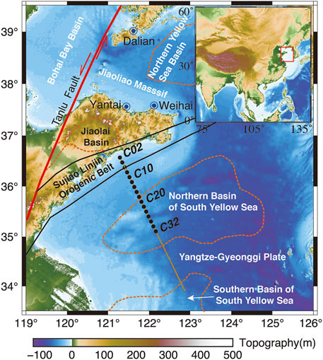
FIGURE 1. Bathymetry/topography of OBS survey line in the Yellow Sea. The line denotes the shot profile, and the black circles denote the OBS deployment locations.
Combined with the shot information, the common receiver gather (CRG) was cut from the raw OBS continuous binary-format data. As an example, the 4C CRGs of the OBS from station number C22 are shown in Figure 2. After obtaining the traces by subtracting their means, a 0.5–6.3 Hz bandpass filter was applied. The pre-processed seismogram shows a body wave (green arrows in Figure 2) with a strong reflection and refraction and a visible Scholte wave (black arrows in Figure 2) for both the seismic components (Figures 2A–C) and hydrophone component (Figure 2D). The raw CRGs also show that the Scholte-wave energy is distributed unevenly between the seismic and hydrophone components. The Scholte-wave energy from the seismic components is stronger than that of the hydrophone component. This may be because the amplitude of the Scholte-wave decays exponentially with distance from the interface, and the geophones of the OBS instrument are directly coupled with the seafloor while the hydrophone floats in the water at 0.8 m from the seabed.
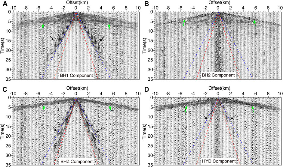
FIGURE 2. Pre-processed common receiver gathers (CRGs) recorded at OBS station C22. Panels (A, B) show two horizontal seismic components with deployed random azimuths. Panels (C, D) show the CRGs of the vertical and hydrophone components, respectively. The red and blue dashed lines denote apparent velocities of 100 and 160 m/s, respectively. The pre-processing involved trace normalization using the mean with bandpass filtering at 0.5–6.3 Hz, and finally Wiener (least-squares) predictive error filtering. The green and black arrows denote the body and Scholte waves, respectively.
The three seismic CRGs show three primary Scholte-wave features. First, both the seismic components and hydrophone component record the Scholte wave. Second, the seismic components with different directions exhibit various energy amplitudes. A dominant Scholte wave is visible in the vertical BHZ component (Figure 2C), whereas a relatively weak Scholte wave is visible in the random-azimuth horizontal BH1 component (Figure 2A) and nearly disappears in the other horizontal BH2 component (Figure 2B). Third, the Scholte wave modes recorded from the different seismic components are distinct, with the BH1 component recording a higher-order mode (Figure 2A) and the BHZ component recording the dominant fundamental mode (Figure 2D).
The OBS 4C Scholte-wave dispersion energy imaging (DEI) and inversion method for each OBS station involved the following four main steps.
Step 1: Preparation of 4C CRGs. Transfer the raw continuous binary OBS data to the 4C CRGs with the SEGY data format, which is followed by pre-processing the raw CRGs with trace normalization, bandpass filtering, Wiener predictive error filtering, and cutting the traces with an absolute offset of 400–5,000 m.
Step 2: 4C DEI. Calculate the velocity spectrum (VS) of each component using a phase-shift algorithm.
Step 3: 4C velocity-spectra stacking. Obtain the final stacked VS by stacking the VSs from the three seismic components with the hydrophone component.
Step 4: Extraction and inversion of the dispersion curve. Pick the multimode dispersion curves from the stacked VS and finally invert the structure for the shallow marine sediment.
As an example, we show the 4C Scholte-wave dispersion analysis method for the OBS station C22. We begin by pre-processing the 4C CRGs following step 1, as shown in Figure 2. The entire CRG is split into two branches: positive and negative offsets. For each CRG branch, the minimum and maximum offset windows are chosen to cut the traces, which guarantees a high signal-to-noise ratio for use in the next step. Here, the near- and far-field effects of the CRG are the primary references used to select the offset window (from 400 to 5,000 m).
The pre-processed CRG branch is then transferred from the t–x domain to the f–v domain using the phase-shift algorithm (Park et al., 1998) following step 2. For one trace of the CRG data
Where
We define a trial phase-velocity (
Where
As shown in Figure 3, the 4C VSs are imaged using the phase-shift algorithm for the positive CRG branch of the OBS station C22. First, the 4C dispersion energy images show that both the seismic and hydrophone components can be used to image the dispersive VSs. Second, both the fundamental mode and higher-order modes are obtained simultaneously. Third, the mode energy is distributed unequally between the different components. The fundamental mode is dominant in the VS of the vertical component (Figure 3C) but missing in those for both horizontal components (Figures 3A,B). Correspondingly, the first higher-order mode is dominant in the two horizontal components. Finally, the recognizable highest dispersive Scholte-wave mode differs between the four components. Thus, the fourth higher-order mode can be distinguished from the BH1 component, the weak third higher-order mode is present in the BHZ component, and the first higher-order mode can be distinguished from the hydrophone component.
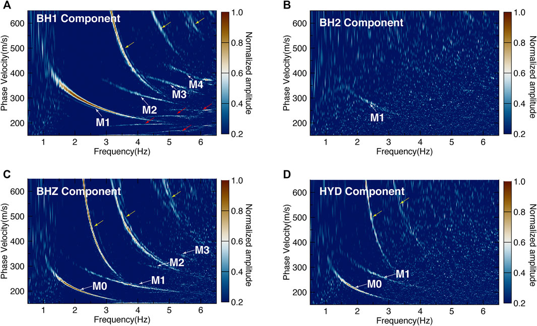
FIGURE 3. Four-component (4C) velocity spectra (VSs) calculated from the positive branch of the 4C CRGs of OBS station C22. The M0–M4 denote the dispersive Scholte-wave mode numbers. The yellow and red arrows denote two different patterns of dispersive spectral-spatial aliasing.
There is a significant difference between the VSs of the two horizontal components; only the first higher-order mode can be recognized from the VS of the BH2 component, whereas the VS of the BH1 component clearly shows the first four higher-order modes. Figure 4 shows hodograms of the BH1-BH2 (Figure 4A) and BH2-BHZ (Figure 4C) components plotted using a time window of 1.7–2.2 s for a seismic trace with an offset of 1,499 m for the OBS station C22. In the BH1-BH2 hodogram, the particle vibration trajectory is characterized as a straight line along the BH1 axis, while the BH2-BHZ particle motion trajectory is a vertical straight line. These two main features of the hodograms indicate that the BH1 component corresponds almost directly to the shot-line azimuth, whereas the BH2 component is perpendicular to the shot line. For this OBS station, BH1 can be treated as the inline component, with BH2 treated as the corresponding crossline component. This explains reasonably well why there is only one relatively weak dispersive energy mode (M1 in Figure 3B) in the VS of BH2.
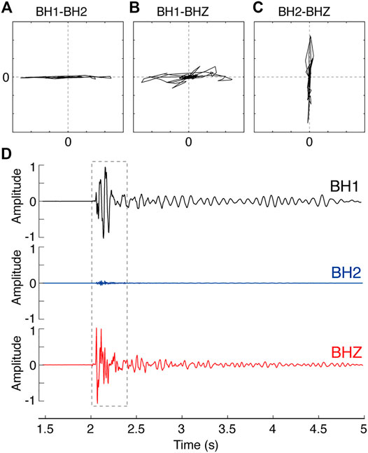
FIGURE 4. Hodograms (A–C) and waveform (D) of the trace with an offset of 1,499 m for OBS station C22. The plotted time window of the hodogram is denoted as the gray dashed rectangle in (D).
We stack the 4C VSs together after completing the above DEI as described in step 3. The 4C stacked VSs (
Where
As an example, the dispersion curves picked from the 4C VSs as shown in Figure 5 are compared in detail. As shown in Figure 5A, the dispersion curves show great consistency between the different components, from the fundamental to the fourth higher-order dispersive modes. The mean of the cross-correlation coefficients between the 4C first-higher-order-mode dispersion curves approaches 99.88%. The correlation coefficient of the first-higher-order-mode dispersion curves produced by the BH1 and BHZ components is the highest and reaches 99.98%. The BH1 and BH2 components have the lowest correlation coefficient of 99.78%, while the other correlation coefficients between BH1 and HYD, BH2 and BHZ, BH2 and HYD, and BHZ and HYD are 99.90, 99.93, 99.80, and 99.88%, respectively. These higher correlation coefficients for the first higher-order mode between different components inversely prove that the dispersive energies come from the same wave source, which is the P-SV type of Scholte wave.
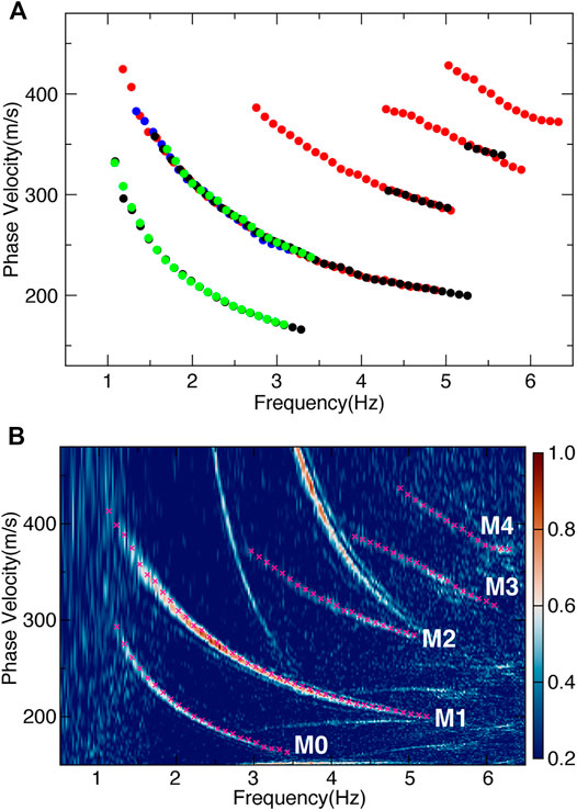
FIGURE 5. Dispersion curves selected from the 4C VSs shown in Figure 3 (A) and the stacked VS (B). The red, blue, black, and green dots in (A) denote the BH1, BH2, BHZ, and HYD components, respectively. The M0–M4 in (B) denote the dispersive mode numbers.
The stacked VS (SVS) is obtained from the normalized 4C VS stacking results. As shown in Figure 5B, the final full-mode SVS can be imaged using the proposed 4C VS stacking method, including the fundamental mode (M0 in Figure 5B) and the first to fourth higher-order modes. Compared with the traditional single vertical component VS, in which only the fundamental and first higher-order modes can be recognized, the fundamental to fourth higher-order modes are observed in the 4C SVS. The missed fundamental mode in the BH1 component appears in the SVS, and the missed second to fourth higher-order modes in the BHZ component are observed from the full-mode SVS.
We directly stack the 4C velocity spectra linearly using the same weights for each component. This approach has the significant advantages of being fast, stable, and effective. To verify whether the weights of the four components affect the extraction of higher-order modes for the Scholte-wave 4C VS stacking method, we chose two sets of random weights as a comparison. We denote the same weight stacking velocity spectrum as
and shown in Figures 6A,B, respectively. All three SVSs show no visible differences and the dispersive characteristics are the same. That is, a total of five modes can be distinguished and the first two lower modes have much stronger energies with the last three higher modes being weaker.
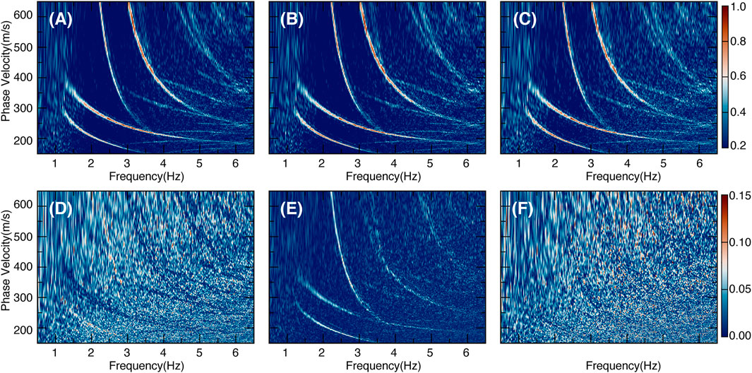
FIGURE 6. The 4C SVS as calculated from different weights (A, B) and the same weight (C). The absolute differences between each SVS pair (A–C) are shown in (D–F).
The absolute difference between every two SVSs is calculated. Thus, the differences between the
The 4C dispersive VS stacking method for Scholte waves can effectively image the full-mode dispersion energy. Compared with the single-vertical-component DEI method, this procedure either increases the number of recognizable higher-order modes or widens the selectable frequency range of the dispersion curves for higher-order modes. For the single-horizontal-component DEI processing, our 4C stacking method entirely avoids mistaken mode misidentification. Thus, the first higher-order mode is treated as the missed fundamental mode in the horizontal component. This also inversely demonstrates the necessity of the 4C Scholte-wave analysis and the failings of the single-component Scholte-wave imaging method.
As shown in Figure 7, all dispersion curves were extracted manually from the 4C SVS of all 14 OBS stations. The manual selection error can be controlled within 5 m/s, which was considered in the subsequent inversion step. The numbers of extracted Scholte-wave modes differ between the OBS stations. Most stations can extract the third higher-order mode, whereas only three stations can extract the fourth higher-order mode. The highest number of extracted modes varies irregularly between the OBSs. A reasonable explanation for this phenomenon of unequal mode numbers is that it is caused by the lateral geological variations in the shallow sediment along the OBS survey line, or by differences in the degree of OBS coupling. Overall, all OBS stations can extract the available multimode dispersion curves for the subsequent inversion procedure.
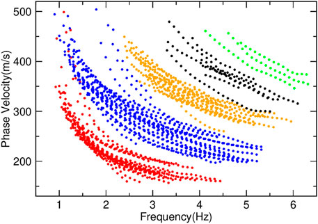
FIGURE 7. All dispersion curves extracted from stacked VSs (SVS) of all OBS stations along the profile. The red, blue, orange, black, and green dots denote the fundamental to fourth higher-order mode, respectively.
The implicit relationship between the earth structure and the dispersion curves is described as (Xia et al., 2003).
Where n is the total number of points on the dispersion curve,
We use the multimode-dispersion-curve joint inversion method (Xia et al., 2003; Luo et al., 2007) to image the geological structures of shallow sediment. The final convergent optimal solution was obtained using the damped iterative least-squares algorithm and was implemented in the Computer Programs in Seismology (CPS) (Herrmann, 2013). During the iterations, only
The initial geophysical model is constructed as an isotropic homogenous water–sedimentary layered model with 40 total layers. For the first sea-water layer,
To determine the deepest constraint depth during inversion, we calculate the sensitivity kernels for the five modes of the Scholte-wave dispersion curves based on the initial geophysical model. As shown in Figure 8,
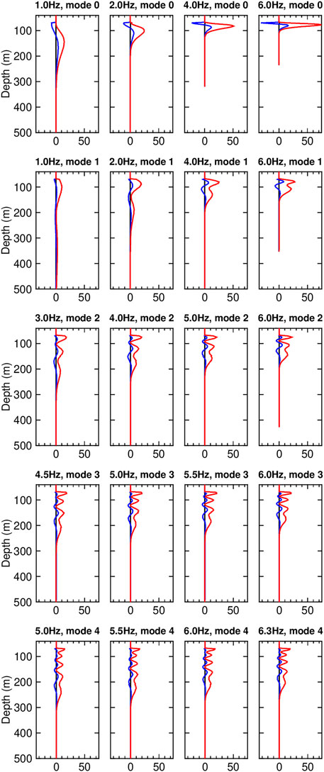
FIGURE 8. Sensitivity kernels of the five dispersive Scholte-wave modes based on the initial marine sedimentary model. The red, blue, and black lines denote the sensitivities of
The sensitivity kernel results illustrate this constraint in Figure 8. The higher-order modes have greater sensitivities to deeper layers than the fundamental mode for the same frequency. For example, when selecting 10% of the mean sensitivity (0.362) as the threshold, the greatest depths for the fundamental to the fourth higher-order mode at 6.0 Hz are 107, 157, 195, 230, 272, and 315 m, respectively. These simple statistical results demonstrate that for the same frequency, the constraint depth of the fourth higher-order mode is 2.94 times that of the fundamental mode. Correspondingly, the higher-order Scholte-wave modes allow “seeing” deeper with an approximately linear trend compared with the fundamental mode. Finally, we choose 10% of the mean sensitivity (0.362) as the threshold to determine the deepest confidence depth for the inverted models, which is 347 m. We first obtain all maximum depth values from the sensitivity kernel of each mode for each frequency based on the threshold (Figure 9), and the final deepest inversion depth is the mean of these maximum depths.
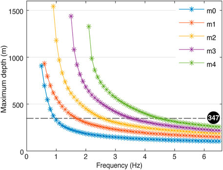
FIGURE 9. The maximum constrained depth obtained from the given threshold of the sensitivity kernel for each mode, where m0–m4 denote the fundamental to fourth-higher-order mode.
We implement the five-mode joint dispersion-curve inversion to obtain the best-fit marine sedimentary model. All modes of the phase-velocity dispersion curves converge well after 20 iterations with a damping factor of 0.1 (Figure 10). The average signal power fit between the inverted and selected dispersion curves for all stations reaches 99.98%. The average standard fitting error for the multimode phase velocities is 4.13 m/s, where the corresponding average fitting residual is 2.46 m/s. The final best-fit
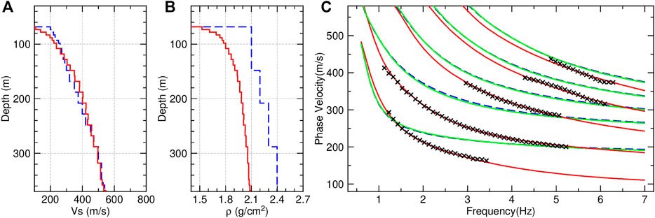
FIGURE 10. Initial (blue dashed line) and best-fit (red solid line) geophysical models of the shear-wave velocity (A) and density (B) from the inverted multimode Scholte-wave dispersion curves (C). The black crosses in (C) denote the picked dispersion curves, the blue dashed line, red solid line, and green solid line denotes the theoretical dispersion curves calculated based on the initial model, the best-fit model, and the best-fit density and initial
In total, 26 dispersion-curve groups were successfully extracted from 13 OBS stations, with one station (C18) having data errors. Of the 26 dispersion-curve groups, three groups extracted a maximum of five modes, five groups extracted a maximum of four modes, 13 groups extracted a maximum of three modes, four groups extracted a maximum of two modes, and one group extracted a maximum of one mode. The phase velocities vary from 150 to 500 m/s for all dispersion-curve groups (Figure 7). The lower velocities belong to classical soft sedimentary geological conditions. Along the survey profile, the Scholte-wave phase velocities show lateral differences, which indicates strong lateral heterogeneity.
All 26 of the 1D shear-wave velocity structures were inverted from the multimode dispersion curves. As shown in Figure 11, the pseudo-2D shear-wave velocity profile was constructed from all the 1D velocity structures. The adjustable tension continuous curvature spline algorithm (Smith and Wessel, 1990) with a tension factor of 0.25 was adopted to interpolate the 1D
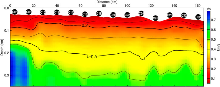
FIGURE 11. Final 2D shear-wave velocity structure of the survey profile. C06–C32 denote the deployed OBS positions.
A large lateral-velocity variation appeared in the constructed 2D S-wave velocity profile. There is a strong high-velocity zone in the middle and deep areas of the northern end (left side of Figure 11) of the survey line, which corresponds to the geological unit of the Qianliyan uplift. The apparent velocity difference between stations C08 and C10 may be indicated as an active fault, which is part of the Qianliyan fault zone (Wu et al., 2020). This corresponds to regional deep large faults with scales that cut through multiple sedimentary layers over a long development time. The
The proposed OBS multicomponent Scholte-wave dispersion analysis method can effectively image the complex, extremely low, and strong lateral velocity variation
In total, 26 dispersion-curve groups were extracted from the negative and positive branches of 13 OBS CRGs in the North Yellow Sea. Lower phase velocities of 150–500 m/s were obtained from all dispersion-curve groups. The damped iterative least-squares algorithm effectively inverted the multimode Scholte-wave dispersion curves (>99.98% goodness-of-fit) based on the water–sedimentary layered homogenous earth model. A maximum inversion-constraint model depth of 350 m was accurately defined by the sensitivity kernel threshold (10% of maximum). The pseudo-2D shear-wave velocity profile was constructed from the 26 1D inverted models. The key geological features of the shallow sediment appeared in the shear-wave velocity profile, including the uplift, active fault, and thrust nappe structures.
The raw data supporting the conclusions of this article will be made available by the authors, without undue reservation.
YW, TH, and QY all contributed as major authors of the manuscript. YW wrote the text, processed the data, and created the figures. TH collected the marine OBS active data and performed the geological interpretation. QY developed the OBS instruments used to collect the seismic data in the study.
This research was funded by the National Natural Science Foundation of China (Grant Nos. 41806083 and 42176084), National Key R&D Program of China (2018YFC0308003), and Major Research Plan on West-Pacific Earth System Multispheric Interactions (project number: 91858212).
The authors declare that the research was conducted in the absence of any commercial or financial relationships that could be construed as a potential conflict of interest.
All claims expressed in this article are solely those of the authors and do not necessarily represent those of their affiliated organizations, or those of the publisher, the editors and the reviewers. Any product that may be evaluated in this article, or claim that may be made by its manufacturer, is not guaranteed or endorsed by the publisher.
The authors thank the crew members and investigators of the Chinese Geophysical Research vessel M/V Discover-2 and Xiangyanghong-2 for collecting the marine seismic data.
Bohlen, T., Kugler, S., Klein, G., and Theilen, F. (2004). 1.5D Inversion of Lateral Variation of Scholte‐wave Dispersion. Geophysics 69 (2), 330–344. doi:10.1190/1.1707052
Bradshaw, A. S., and Baxter, C. D. (2015). Measurement of Shear Wave Velocity in marine Sediments. The J. Acoust. Soc. America 137, 2284. doi:10.1121/1.4920337
Dong, H., Nguyen, T.-D., and Duffaut, K. (2012). Estimation of Shear-Velocity Profiles Using Shear Source Data in marine Environment. J. Acoust. Soc. America 131, 3278. doi:10.1121/1.4708258
Du, S., Cao, J., Zhou, S., Qi, Y., Jiang, L., Zhang, Y., et al. (2020). Observation and Inversion of Very-Low-Frequency Seismo-Acoustic fields in the South China Sea. J. Acoust. Soc. America 148 (6), 3992–4001. doi:10.1121/10.0002949
Ewing, J., Carter, J. A., Sutton, G. H., and Barstow, N. (1992). Shallow Water Sediment Properties Derived from High-Frequency Shear and Interface Waves. J. Geophys. Res. 97 (B4), 4739. doi:10.1029/92JB00180
Herrmann, R. B. (2013). Computer Programs in Seismology: An Evolving Tool for Instruction and Research. Seismological Res. Lett. 84 (6), 1081–1088. doi:10.1785/0220110096
Hughes, S. J., Ellis, D. D., Chapman, D. M. F., and Staal, P. R. (1990). Low‐frequency Acoustic Propagation Loss in Shallow Water over Hard‐rock Seabeds Covered by a Thin Layer of Elastic-Solid Sediment. J. Acoust. Soc. America 88 (1), 283–297. doi:10.1121/1.399951
Klein, G., Bohlen, T., Theilen, F., Kugler, S., and Forbriger, T. (2005). Acquisition and Inversion of Dispersive Seismic Waves in Shallow marine Environments. Mar. Geophys. Res. 26, 287–315. doi:10.1007/s11001-005-3725-6
Kugler, S., Bohlen, T., Bussat, S., and Klein, G. (2005). Variability of Scholte-Wave Dispersion in Shallow-Water marine Sediments. Jeeg 10 (2), 203–218. doi:10.2113/JEEG10.2.203
Kugler, S., Bohlen, T., Forbriger, T., Bussat, S., and Klein, G. (2007). Scholte-wave Tomography for Shallow-Water marine Sediments. Geophys. J. Int. 168, 551–570. doi:10.1111/j.1365-246X.2006.03233.x
Li, W., Lu, W., Liu, Y., and Xu, J. (2012). Superimposed versus Residual basin: the North Yellow Sea basin. Geosci. Front. 3 (1), 33–39. doi:10.1016/j.gsf.2011.11.001
Love, A. E. H. (1911). Some Problems of Geodynamics. Cambridge University Press: Cambridge University Press.
Luo, Y., Xia, J., Liu, J., Liu, Q., and Xu, S. (2007). Joint Inversion of High-Frequency Surface Waves with Fundamental and Higher Modes. J. Appl. Geophys. 62 (4), 375–384. doi:10.1016/j.jappgeo.2007.02.004
Nguyen, X. N., Dahm, T., and Grevemeyer, I. (2009). Inversion of Scholte Wave Dispersion and Waveform Modeling for Shallow Structure of the Ninetyeast Ridge. J. Seismol 13 (4), 543–559. doi:10.1007/s10950-008-9145-8
Park, C. B., Miller, R. D., and Xia, J. (1998). “Imaging Dispersion Curves of Surface Waves on Multi‐channel Record,” in SEG Technical Program Expanded Abstracts, 1377–1380. doi:10.1190/1.1820161
Rauch, D. (1980). Experimental and Theoretical Studies of Seismic Interface Waves in Coastal Waters. Bottom-Interacting Ocean Acoust. 53, 307–327. doi:10.1007/978-1-4684-9051-0_21
Scholte, J. G. (1947). The Range of Existence of Rayleigh and Stoneley Waves. Geophys. J. Int. 5, 120–126. doi:10.1111/j.1365-246X.1947.tb00347.x
Shtivelman, V. (2004). Estimating Seismic Velocities below the Sea-Bed Using Surface Waves. Near Surf. Geophys. 2 (4), 241–247. doi:10.3997/1873-0604.2004021
Shtivelman, V. (2003). Using Surface Waves for Studying the Shallow Subsurface. Bollettino di Geofisica Teorica en Applicata 44 (3), 223–236.
Smith, W. H. F., and Wessel, P. (1990). Gridding with Continuous Curvature Splines in Tension. Geophysics 55 (3), 293–305. doi:10.1190/1.1442837
Socco, V. L., Boiero, D., Maraschini, M., Vanneste, M., Madshus, C., Westerdahl, H., et al. (2011). On the Use of the Norwegian Geotechnical Institute's Prototype Seabed-Coupled Shear Wave Vibrator for Shallow Soil Characterization - II. Joint Inversion of Multimodal Love and Scholte Surface Waves. Geophys. J. Int. 185, 237–252. doi:10.1111/j.1365-246X.2011.04961.x
Vanneste, M., Madshus, C., Socco, V. L., Maraschini, M., Sparrevik, P. M., Westerdahl, H., et al. (2011). On the Use of the Norwegian Geotechnical Institute's Prototype Seabed-Coupled Shear Wave Vibrator for Shallow Soil Characterization - I. Acquisition and Processing of Multimodal Surface Waves. Geophys. J. Int. 185 (1), 221–236. doi:10.1111/j.1365-246X.2011.04960.x
Wang, Y., Li, Z., Geng, J., You, Q., Hao, T., Hu, Y., et al. (2020). Seismic Imaging of S-Wave Structures of Shallow Sediments in the East China Sea Using OBN Multicomponent Scholte-Wave Data. Geophysics 85 (6), EN87–EN104. doi:10.1190/geo2019-0639.1
Wang, Y., Li, Z., You, Q., Hao, T., Xing, J., Liu, L., et al. (2016). Shear-wave Velocity Structure of the Shallow Sediments in the Bohai Sea from an Ocean-Bottom-Seismometer Survey. Geophysics 81 (3), ID25–ID36. doi:10.1190/geo2015-0417.1
Wu, D., Zhu, X., Wang, Q., and Hou, F. (2020). Characteristics of Active Faults Related to Deep Faults in the north Western Part of the South Yellow Sea (In Chinese). Mar. Geology. Front. 36 (2), 12–18. doi:10.16028/j.1009-2722.2019.039
Xia, J., Miller, R. D., Park, C. B., and Tian, G. (2003). Inversion of High Frequency Surface Waves with Fundamental and Higher Modes. J. Appl. Geophys. 52 (1), 45–57. doi:10.1016/S0926-9851(02)00239-2
Zhao, M., Qiu, X., Xia, S., Wang, P., Xia, K., and Xu, H. (2008). Identification and Analysis of Shear Waves Recorded by Three-Component OBSs in Northeastern South China Sea. Prog. Nat. Sci. 18, 181–188. doi:10.1016/j.pnsc.2007.06.005
Keywords: Scholte wave, shear-wave velocity, OBS, dispersion curves, higher-modes
Citation: Wang Y, You Q and Hao T (2022) Estimating the Shear-Wave Velocities of Shallow Sediments in the Yellow Sea Using Ocean-Bottom-Seismometer Multicomponent Scholte-Wave Data. Front. Earth Sci. 10:812744. doi: 10.3389/feart.2022.812744
Received: 10 November 2021; Accepted: 05 January 2022;
Published: 24 January 2022.
Edited by:
Nicola Alessandro Pino, National Institute of Geophysics and Volcanology (INGV), ItalyReviewed by:
Stefania Danesi, Istituto Nazionale di Geofisica e Vulcanologia (INGV), ItalyCopyright © 2022 Wang, You and Hao. This is an open-access article distributed under the terms of the Creative Commons Attribution License (CC BY). The use, distribution or reproduction in other forums is permitted, provided the original author(s) and the copyright owner(s) are credited and that the original publication in this journal is cited, in accordance with accepted academic practice. No use, distribution or reproduction is permitted which does not comply with these terms.
*Correspondence: Yuan Wang, eXdhbmdAbWFpbC5pZ2djYXMuYWMuY24=; Tianyao Hao, dHloYW9AbWFpbC5pZ2djYXMuYWMuY24=
Disclaimer: All claims expressed in this article are solely those of the authors and do not necessarily represent those of their affiliated organizations, or those of the publisher, the editors and the reviewers. Any product that may be evaluated in this article or claim that may be made by its manufacturer is not guaranteed or endorsed by the publisher.
Research integrity at Frontiers
Learn more about the work of our research integrity team to safeguard the quality of each article we publish.