 Cristin L. Wright
 Carl T. Friedrichs
94% of researchers rate our articles as excellent or good
Learn more about the work of our research integrity team to safeguard the quality of each article we publish.
Find out more
ORIGINAL RESEARCH article
Front. Earth Sci., 14 March 2022
Sec. Marine Geoscience
Volume 10 - 2022 | https://doi.org/10.3389/feart.2022.805130
This article is part of the Research TopicCohesive Sedimentary Systems: Dynamics and DepositsView all 21 articles
The objectives of this study are to better understand controls on bed erodibility in muddy estuaries, including the roles of both sediment properties and recent hydrodynamic history. An extensive data set of erodibility measurements, sediment properties, and hydrodynamic information was utilized to create statistical models to predict the erodibility of the sediment bed. This data set includes >160 eroded mass versus applied stress profiles collected over 15 years along the York River estuary, a system characterized by “depth-limited erosion,” such that the critical stress for erosion increases rapidly with depth into the bed. For this study, erodibility was quantified in two ways: the mass of sediment eroded at 0.2 Pa (a stress commonly produced by tides in the York), and the normalized shape of the eroded mass profile for stresses between 0 and 0.56 Pa. In models with eroded mass as the response variable, the explanatory variables with the strongest influence were (in descending order) tidal range squared averaged over the previous 8 days (a proxy for recent bottom stress), salinity or past river discharge, sediment organic content, recent water level anomalies, percent sand, percent clay, and bed layering. Results support the roles of 1) recent deposition and bed disturbance increasing erodibility and 2) cohesion/consolidation and erosion/winnowing of fines decreasing erodibility. The most important variable influencing the shape of the eroded mass profile was eroded mass at 0.2 Pa, such that more (vs. less) erodible cases exhibited straighter (vs. more strongly curved) profiles. Overall, hydrodynamic variables were the best predictors of eroded mass at 0.2 Pa, which, in turn, was the best predictor of profile shape. This suggests that calculations of past bed stress and the position of the salt intrusion can serve as useful empirical proxies for muddy bed consolidation state and resulting erodibility of the uppermost seabed in estuarine numerical models. Observed water content averaged over the top 1 cm was a poor predictor of erodibility, likely because typical tidal stresses suspend less than 1 mm of bed sediment. Future field sampling would benefit from higher resolution observations of water content within the bed’s top few millimeters.
High sediment bed erodibility can lead to a number of ecological and societal complications within an estuarine or coastal system. Ecological implications relating to high bed erodibility include bed disturbance influencing benthic community structure (Schaffner et al., 2001) and increased suspended sediment concentrations decreasing photosynthesis (Cloern, 1987; Kruk et al., 2015). Additionally, sorption of harmful contaminants and excess nutrients to fine-particles can cause re-introductions of these pollutants during sediment erosion, which can lead to harmful bioaccumulation (Yujun et al., 2008) or increased nutrient loadings within a system (Moriarty et al., 2021). Aside from ecological complications, societal ramifications of high sediment bed erodibility relate to infilling of shipping channels (Brouwer et al., 2018) and potential burial or exposure of dangerous unexploded ordinance (Cooper and Cooke, 2018).
Sediment bed erodibility describes how susceptible sediment is to being entrained into suspension in response to the bed stress (τb) caused by the movement of the water immediately above the bed. The more sediment mass a given stress erodes in a given amount of time, the greater the bed erodibility. A widely applied equation for predicting the rate of fine sediment mass eroded into suspension as a function of bed stress is the Ariathurai-Partheniades equation (e.g., Mehta, 2014):
where E is the sediment mass erosion rate, z is depth into the bed, τc is the critical stress for erosion of the sediment, and M is the empirical erosion rate parameter which linearly relates the excess shear stress (τb–τc) to the observed erosion rate, E. Assuming that Eq. 1 holds, then observations of E as a function of τb can be used to determine best-fit values for τc and M, which then quantifies the sediment’s erodibility.
When applying Eq. 1 to many natural estuarine environments, it is helpful to recognize the endmember case of “depth-limited” erodibility that is characterized by values of τc that increase rapidly with depth into the bed (Sanford and Maa, 2001; Rinehimer et al., 2008). In that case, if a continuous, constant bed stress (τb) is applied that is greater than the surface value of τc, the total amount of sediment eventually eroded in a given “long” period of time depends only on (and is limited by) the depth into the bed at which τc = τb. The value of M does not matter. The “long” period of time needed for this adjustment to τc ≈ τb in muddy tidal estuaries with moderate sediment concentrations (10–100 s of mg/L) is commonly as little as 15 min, which is effectively instantaneous relative to the timescale of a tidal cycle (Sanford and Maa, 2001). This means that in such systems, one can quantify and, ultimately, predict the erodibility of the sediment bed simply by quantifying and modeling the τc profile, without needing to model the behavior of M.
The magnitude of erodibility can be influenced by physical, geochemical, and biological sediment properties and processes (Grabowski et al., 2011). Sediment bulk density (or conversely, sediment water content) is often found to be a prominent physical property influencing erodibility of mud (e.g., Jepsen et al., 1997; Roberts et al., 1998; Mehta, 2014). Grain size and minerology can also affect sediment erodibility. For sand, a decrease in grain size increases erodibility. But for muds, a further decrease in grain size below medium silt (∼20 microns) tends to decrease erodibility (Roberts et al., 1998; Grabowski et al., 2011; Mehta, 2014). However, erodibility trends for mixed grain sediment can be more complex (Barry et al., 2006; Jacobs et al., 2011; Wu et al., 2018). With regards to mud composition, muds rich in more cohesive clays, such as smectite, are generally less erodible than those rich in less cohesive clays, such as kaolinite (Mehta, 2014). Higher organic content of seabed mud is commonly associated with biofilms that stabilize the bed and decrease erodibility, especially on intertidal flats (e.g., Andersen, 2001; Lucas et al., 2003; Zhu et al., 2019). Alternatively, a positive relationship between organic content and erodibility may indicate the presence of freshly deposited flocs rather than older, more consolidated muds (Dickhudt et al., 2009; Kraatz, 2013). The relationship between sediment erodibility and bioturbation has been reported to both increase and decrease sediment stability, depending on species and grain size present (Li et al., 2017; Cozzoli et al., 2019) and the burrowing and feeding style of the organisms (Luckenbach, 1986; Grabowski et al., 2011). For example, compaction of loose muddy flocs into denser, resilient pellets by suspension-feeding polychaetes increases the settling velocity of mud aggregates while decreasing their cohesion, which could increase or decrease their ease of resuspension (Haven and Morales-Alamo, 1968; Kraatz, 2013).
Although sediment properties and biological influences are locally important in determining erodibility, it is hydrodynamic forces that ultimately create bottom stresses and circulation patterns that determine the patterns of recent erosion and deposition that then influence subsequent erodibility (Sanford, 2008; Brouwer et al., 2018). Increasing or decreasing tidal range over the past several days has been shown to influence bed erodibility (Kraatz, 2013; Huang et al., 2020), presumably due to its correlation with recent tidal bed stress and associated bed disturbance. Patterns of erodibility within a partially-mixed estuary can also be related to location within the estuary and position along the salinity gradient (Dickhudt et al., 2009; Burchard et al., 2018). In stratified estuaries, higher (or lower) river discharge changes the salinity distribution and locations of sediment transport convergence, pushing easily suspended pools of mud down (or up) the system. Analogous along-channel migrations of highly erodible deposits are seen in well-mixed estuaries in response to temporally-varying competitions between tidal asymmetry and river discharge (Friedrichs et al., 1998; Brouwer et al., 2018).
In this study, we build upon previous findings regarding controls on estuarine sediment bed erodibility by empirically analyzing an extensive set of erodibility data collected over the last 15 years in the York River estuary, VA, United States. Our goal is to investigate the relative importance of various sediment properties and environmental forcings in predicting bed erodibility in a representative muddy, moderately turbid, partially-mixed, tidal estuary. In the following section, the estuarine setting of the study is reviewed, followed by a presentation of data collection and analysis methods, including the multiple linear regression approach used to rank the relative importance of the explanatory variables. Next, results are presented for linear models that predict 1) the total mass erosion at a characteristic bed stress (0.2 Pa) reached during most tidal cycles and 2) the normalized shape of the eroded mass profile as a function of applied bed stress from 0 to 0.56 Pa. Finally, the last two sections provide a discussion and summary of the study’s most important findings, their implications, and directions for future work.
The York River estuary (Figure 1) is an opportune location for examining years of available observations of erodibility to statistically investigate the relative importance of multiple factors that may influence estuarine bed erodibility. Numerous individual studies involving erodibility measurements have focused on this estuary (Friedrichs et al., 2008; Cartwright et al., 2009; Dickhudt et al., 2009; Fall, 2012; Kraatz, 2013; Bilici et al., 2019; Massey et al., 2019), taking advantage of its relatively wide range of environmental conditions, as well as its convenient proximity to the Virginia Institute of Marine Science. Along with this, a variety of research has been conducted in the York aligning with the motivations highlighted in the introduction, such as benthic organism communities and sediment interactions (Schaffner et al., 2001; Hinchey, 2002; Gillett and Schaffner, 2009) and sediment effects on water clarity and light limitation of primary production (Moore et al., 1997; Sin et al., 1999; Reay, 2009; Fall, 2020).
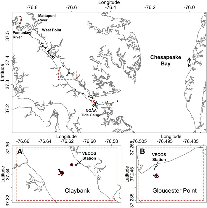
FIGURE 1. Map of the field setting. Red circles are coring locations. (A) and (B) indicate Claybank and Gloucester Point coring areas.
The York River, which is a tidally-dominated, partially-mixed estuary, is one of the major tidal tributaries of the Chesapeake Bay and is formed at its head by two additional tidal tributaries, the Pamunkey and the somewhat smaller Mattaponi (Figure 1). Although its tidal range (0.7 m at the York’s mouth, increasing to 1 m in the upper Pamunkey) defines the system as microtidal, the tidal current along the estuary can reach 1 m/s at spring tide (Schaffner et al., 2001; Friedrichs, 2009). The impact of wind waves is generally limited to quite shallow water (<∼2-m depth), given that the mean wave period is only 1.9 s, and significant wave heights exceed 0.3 m only 1% of the time (Vandever, 2007). Nonetheless, winds are still important to mean currents in deeper water, with the typical pattern of estuarine circulation enhanced or reduced by down- or up-estuary winds, respectively (Scully et al., 2005). The main channel that reaches from the mouth to West Point ranges in depth from 6 to 20 m, deepening towards the mouth, and salinity stratification increases seaward in response to the depth increase. There is also a 5-m deep secondary channel that runs from Gloucester Point to Claybank that is separated from the main channel by a shallow channel-parallel shoal (Schaffner et al., 2001; Friedrichs, 2009). The salt intrusion limit for the York River—Pamunkey River system lies between 40 and 90 km upstream of the York River mouth and moves up and downriver with fluctuations in river discharge.
The areas of highest erodibility along the York tend to mirror the region of the estuary containing its main estuarine turbidity maximum (ETM) and secondary turbidity maximum (STM) (Dickhudt et al., 2009). Thus, understanding large-scale controls on bed erodibility in the York requires understanding the dynamics of the STM and ETM. The main ETM in the York (Figure 2) follows the migration of the salt intrusion limit and is formed largely by a decrease in the strength of near-bed estuarine circulation with distance upstream, which traps easy to resuspend sediment in the upper estuary (Lin and Kuo, 2001; Friedrichs, 2009). In addition to the ETM, a seasonal secondary turbidity maximum (STM) is often observed in the York River, with the downstream extent falling in the Claybank region, 30 km from the mouth (Figure 2) (Lin and Kuo, 2001). The STM tends to be more intense during times of high river discharge and low salinity (Lin and Kuo, 2001; Dickhudt et al., 2009). The STM is formed by similar mechanisms as the ETM, but is located downstream of the salt intrusion limit, at a transition zone between the shallower, more well-mixed water column upriver, and the deeper, more stratified water column downriver (Lin and Kuo, 2001). The STM and ETM in the York are more intense at spring tide than neap tide, but their along-channel locations do not notably change at spring versus neap (Lin and Kuo, 2001).
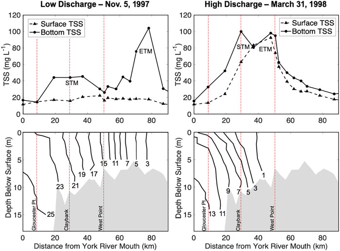
FIGURE 2. Total suspended solids (TSS) collected 1-m below the surface and 1-m above the bottom (top panels) and salinity contours (bottom panels) along the York River estuary during low river discharge (left panels) and high river discharge (right panels) Adapted by permission from Springer Nature, Estuaries (Lin and Kuo, 2001), copyright 2001.
Grain-size distributions of the sediment bed of the York are largely dependent on location and water depth. The upper and mid-river locations have high percentages of mud (>80% mud) in the tidal channels with sediments coarsening (<40% mud) on the narrow shoals and along the shoal between the primary and secondary channels (40–80% mud) (Nichols et al., 1991). In the lower river, the main channel remains muddy (>80% mud), but with broad, sandy shoals with coarser sediment (<40% mud) (Nichols et al., 1991).
Erodibility data, along with a suite of sediment and water column parameters, were collected from cores over 160 times in the York River—Pamunkey River system (Figure 1) between 2005 and 2019. A GOMEX box core (surface area 625 cm2) was collected at each location, and then multiple 10-cm diameter sub-cores were collected by hand from the box core. These sub-cores were used for analysis of erodibility and for determining disaggregated sediment grain size, resilient pellet content, organic content, and water content. For this project, parameter values from only the top centimeter were used. Disaggregated fractions of sand (>63 μm), silt (63 to 4 μm), and clay (<4 μm) by mass were determined by sonification followed by a combination of wet sieving and pipette analysis. Starting in 2010, resilient fecal pellet abundance was determined by wet sieving untreated sediment following the methods of Kraatz (2013). This involved first using a 63-μm sieve to isolate sand plus resilient sand-sized mud pellets and then subtracting out the previously calculated disaggregated sand component. More details regarding steps in the field data collection and laboratory analysis are provided in Wright (2021).
Sediment erodibility at each location was evaluated using a Gust microcosm (e.g., Dickhudt et al., 2009). During erodibility analysis, a sediment core is topped with a specially designed cap that is equipped with a rotating disk. The disk spins at varying speeds to create known stresses on the sediment bed while site water is pumped through the core. The water pumped out of the core is analyzed for turbidity and then filtered for suspended solids, and the calibrated turbidity time series is used to determine the mass of sediment eroded at each applied stress (Figure 3A). After a 30-min initial interval at 0.01 Pa, the stress is increased stepwise from 0.02 to 0.56 Pa, each lasting 20 min. These stresses are within the range of natural shear stresses observed in the York River in response to typical tidal and fluvial processes (Figure 3B).
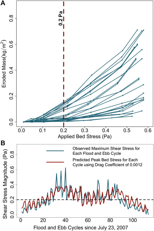
FIGURE 3. (A) Examples of interpolation at 0.2 Pa of erosion curves from the Gust microcosm experiments. (B) Bottom shear stress observed in the Claybank region of the York River (Fall, 2012) along with bed stress estimated from τb = CD U2, where U is cross-sectionally averaged tidal velocity amplitude (see Section Quantifying the Erodibility Profile).
Water content of each sediment sample by mass was determined by calculating the difference in mass from wet weight and dry weight after being thoroughly dried in an oven at 103–105°C. Due to most samples having high contents of mud, the percent water of the mud portion [100 × water mass/(water + dry mud mass)] was used instead of percent water of the total sample, similar to analysis performed by Dickhudt et al. (2011). The logic behind this approach is that at high mud content (when interlocking sand grains are not supporting the weight of the sediment), the most relevant role of water is to indicate the compaction of the mud matrix, not the compaction of the sand. The samples used for percent water were then muffled at 550°C to determine percent organic based on loss on ignition.
In the majority of cases, a 11.5 cm by 2.5 cm rectangular sub-core was also collected for X-radiography, and the resulting X-ray images were manually sorted into two categories. One category included samples that had a clearly mottled fabric (Figure 4A), and the other category included those that were laminated (Figure 4B) or that had a distinct low-density deposit layer at the surface (Figure 4C). Because 1) there were individually far fewer cases that were either laminated or that had a detectable surface layer relative to those that displayed mottling up to the surface, and 2) the hypothesized meaning of lamination or layering was similar (i.e., recent net deposition without time for extensive bioturbation), the laminated and surface layer categories were combined into one “layered” category. “Layered” vs. “Not layered” (i.e., mottled) was then included as an explanatory variable in model runs.
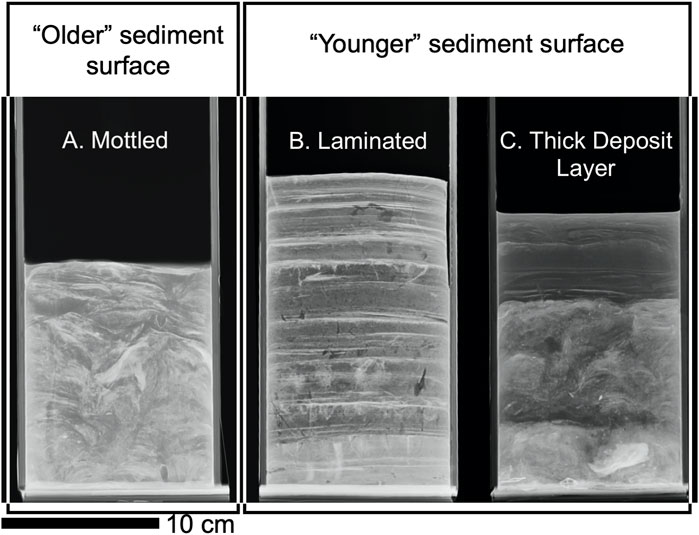
FIGURE 4. X-ray images representing (A) mottled, (B) laminated, and (C) thick deposit layer fabrics. These “negative” images are darker where wet sediment density is lower. The laminated and deposit layer classes were combined and likely represent younger near-surface sediments, whereas the mottled class likely represents older near-surface sediments.
It is important to note that on each sampling cruise, a Gust erodibility sub-core was typically collected from each of two consecutive box cores, and the two sub-cores were then each analyzed by the Gust microcosm. The two box cores were usually collected on the order of a few to 10 s of meters apart, as dictated by the boat’s movement around its anchor point, typically close to slack tide. Two sediment property sub-cores were taken (one from each box core), and sediment from corresponding depths from both cores were combined for an average for the location. Because of this, many of the Gust experiment data have independent erodibility measurements but identical grain size, percent organic, percent water, and pellet content for a single sampling station. Limitations of sampling approaches in this study with regards to the interpretation of statistical analyses are further addressed in the discussion section.
In the depth-limited erodibility extreme, which has been found to apply very well to the muddy bed of the York River estuary (Rinehimer et al., 2008; Cartwright et al., 2009; Dickhudt et al., 2011; Fall, 2012), the sediment’s critical stress profile (τc) alone is sufficient to fully quantify its erodibility. As surficial sediment is removed during active bed erosion in estuaries like the York, the magnitude of τc at the newly exposed, underlying bed surface typically approaches the value of the bed stress (τb) imposed by the overlying flow within ∼15 min (Sanford and Maa, 2001). This means that at the end of each of the 20–30 min periods of constant stress utilized by the Gust microcosm on cores from the York as τb was increased incrementally from 0.01 to 0.56 Pa, one could assume that τc ≈ τb. The corresponding mass of sediment eroded at each of these levels of τc ≈ τb was known from integrating the flow rate through microcosm times the recorded time-series of suspended sediment concentration. Thus, the vertical profile of τc as a function of eroded mass was successfully quantified.
The next step was to condense the information provided by the τc profile at each site (i.e., seven eroded masses at seven corresponding values of τb) into just two values, one representing the overall magnitude of erodibility, and the other representing the shape of the τc profile. Each of these values was used as a response variable in subsequent statistical models. The first response variable was chosen to be the mass of sediment that had been eroded at a single representative bed stress common to all of the Gust microcosm experiments (and also characteristic to typical tidal flows in the York). The second response variable was obtained by using the dominant component of a principal component analysis to describe the erosion profile shape.
As noted above, the first erodibility response variable was the mass of sediment that had been eroded at a specific applied bed stress. In this study, the cumulative eroded mass at 0.2 Pa was interpolated and used as the characteristic eroded mass value for each Gust erosion experiment (Figure 3A). Based on observations of τb from acoustic Doppler velocimeters (ADVs), previous investigators have identified τb = 0.2 Pa as a representative tidal stress for the York River estuary (Friedrichs et al., 2008; Fall, 2012; Kraatz, 2013). For example, Fall (2012) found that during the summer of 2007 (Figure 3B), τb during that time often reached ∼0.2 Pa during peak flood and ebb flows, with a few maximum stresses reaching ∼0.5–0.6 Pa. Similar magnitudes for τb can be found for each tide based on the analytical solution for the amplitude of cross-sectionally averaged tidal velocity (U) in a long, straight channel with weak friction (Friedrichs, 2010):
where RT is the observed range between each low and high tide, g = 9.8 m/s2, <h> is spatially- averaged water depth, and τb = CD U2. For the York, <h> ≈ 6 m (Nichols et al., 1991; Friedrichs, 2009), and CD ≈ 0.0012 based on the ADV measurements of Fall (2012) (Figure 3B).
In channelized tidal estuaries such as the York-Pamunkey system, the amplitude of tidal shear stress associated with a given tidal range is often relatively uniform for long distances along the main tidal channels. For example, observations by Cartwright et al. (2009) found a similar range of τb at both Gloucester Point and Claybank during several months of ADV deployments, and 3-D modeling by Fall et al. (2014) calculated relatively similar τb in channels along the York in both downstream and upstream locations. Thus, tidal range squared at a given time is expected to be approximately proportional to the amplitude of τb within channels along much of the system. Morphodynamics favors relatively uniform peak tidal velocity and τb along channelized tidal estuaries in general, and this pattern has been noted along additional systems such as the Delaware, Gironde, Hudson, James, Thames, and many others (Friedrichs, 1995; Lanzoni and Seminara, 2002; Olabarrita et al., 2018).
Erodibility was also quantified by the shape of the eroded mass profile. Profiles for each Gust experiment were compiled (Figure 5) and analyzed using principal component analysis (PCA) to determine the shape of the most common deviation for the mean profile. Eroded masses for τb = 0.01, 0.05, 0.1, 0.2, 0.3, 0.45, and 0.56 Pa were interpolated for each profile produced by the Gust experiments (Figure 5A). When profiles did not reach τb = 0.56 Pa, but the final experimental stress point exceeded 0.50 Pa, the last data point was linearly extrapolated. All Gust erosion profiles were divided by the mass eroded at τb = 0.56 Pa, resulting in a normalized erosion profile shape constrained between 0 and 1 (Figure 5B). The normalized values were then averaged across all the profiles, and the average normalized profile was subtracted from the individual normalized profiles to center the data around a global mean of zero (Figure 5C). Finally, the deviations from the average normalized profile were used as input to the PCA. Similar PCA methods for describing profile shapes have been used for the topography of tidal flats and are described in Bearman et al. (2010). Note that for this analysis, some Gust experiments did not have applied τb exceeding 0.45 Pa. These profiles were removed (see Wright et al., 2021 for a list of the removed profiles), which created a slightly smaller data subset for this response variable relative to the set for eroded mass at τb = 0.2 Pa. Figures 5D–F display the output of the PCA analysis, which is described in the results section.
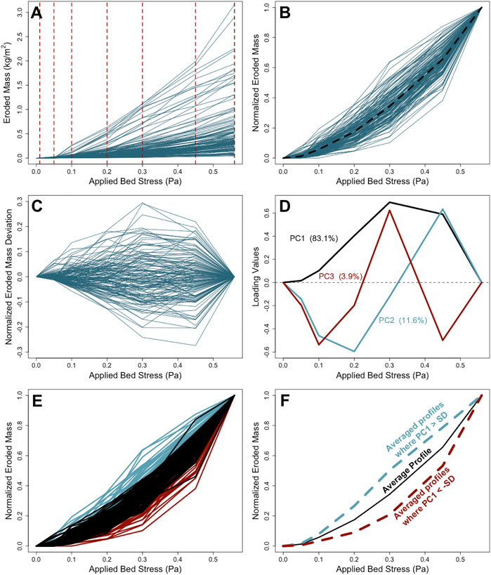
FIGURE 5. Erosion profile shape normalization process. (A) Interpolated Gust output data with interpolation points highlighted by dashed red lines. Each profile in (A) was divided by its eroded mass value at 0.56 Pa, resulting in normalized erosion shapes bounded between 0 and 1 in panel (B). The average profile in (B) (dashed black line) was subtracted from all normalized profiles to center the data around zero in (C). (D) Loading values for PC1, PC2, and PC3 determined from (C) for the All Sites data subset. (E) All Sites profile shapes with PC1 scores within ± 1 standard deviation (SD) of zero (black), PC1 > 1 SD (blue), and PC1 < -1 SD (red). (F) Average profile shapes for all normalized profiles in (E), for those with PC1 > 1 SD, and for those with PC1 < -1 SD.
Observed and predicted tidal ranges were downloaded from the National Oceanic and Atmospheric Administration (NOAA, 2021) for the tide gauge located at the Yorktown Coast Guard pier (see Figure 1) to provide a variable proportional to the amplitude of the tidal current. Tidal ranges are defined as the absolute difference between each high tide and its preceding low tide and vice versa; so, each day includes an average of 3.9 tidal ranges. The observed tidal ranges were then squared to transform that variable into one proportional to the amplitude of the tidal bed stress. Time series of tidal range squared prior to each box core collection were used to produce running averages of progressively increasing length, preceding the timing of each associated erodibility measurement. The preceding running average length that produced the highest correlation between past tidal range squared and eroded mass at 0.2 Pa was then used for calculating the tidal range squared explanatory variable. In addition to observed tidal ranges, the absolute difference between NOAA predicted and observed tidal ranges was recorded, which here is termed the water level anomaly. This variable was used to determine if meteorological events that drive relatively rapid changes in set-up or set-down of water level along the estuary influence sediment erodibility. The water level anomaly was likewise put through a series of preceding running averages of increasing length, and the case with the best correlation with eroded mass at 0.2 Pa was retained as the water level anomaly explanatory variable.
River discharge and salinity were also compiled for use as explanatory variables. Changing discharge and salinity are expected to serve as proxies for the movement of temporary, highly erodibility mud deposits which migrate, up- and down-river in concert with the ETM and STM. Daily river discharge data were downloaded from the United States Geological Survey (USGS, 2021) and summed for the two main tributaries of the York River: the Pamunkey and Mattaponi. An approach similar the treatment to tidal range and water level anomaly was used to create an optimal running average of river discharge prior to sampling of eroded mass. Salinity data for erodibility samples collected at Claybank and Gloucester Point were downloaded from the Virginia Estuarine and Coastal Observing System (VECOS, 2021) stations (see Figure 1) that are also located near Claybank and Gloucester Point. Because short-term salinity variation was high due to tidal advection, the previous 25 h before sampling (the approximate length of two M2 tidal constituent cycles) was averaged for each set of VECOS salinity readings and used for data analysis. For sample sites not located in close proximity to the VECOS buoys (only 26 out of ≥160 erodibility measurements), depth-averaged salinity collected at the coring site at the time of sampling was used as a best available estimate of the recent characteristic salinity.
Different data subsets with increasingly more common attributes (and smaller sample size) were created and were explored with multiple statistical methods (Table 1). The entire data set included 167 erodibility profiles collected at various locations (see Figure 1) along the York River system (which here includes the lower Pamunkey). The means, standard deviations, and ranges for the entire data set are provided in Table 2. Two of the 167 data points were found to be extreme outliers in all models over the course of model exploration and were removed from further model-fitting. [A complete listing of all data points and their individual properties are provided in Wright et al. (2021)]. The first data subset analyzed statistically included all the remaining observations (n = 165). Most samples were located below the ETM except those in the Pamunkey River. The next data subset removed the Pamunkey River samples and only contained the fully “estuarine” sites (i.e., sites located seaward of the transition to fresh water) (n = 158), the logic being that distinct physical processes (such as density-driven estuarine circulation) occur in brackish conditions.
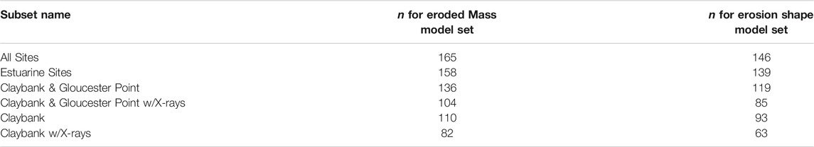
TABLE 1. List of data subset names and sample sizes for the Eroded Mass Model Set and the Erosion Shape Model Set.
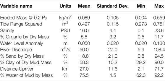
TABLE 2. Data and variance statistics for variables prior to log transformation or standardization, but after low-pass averaging recent tidal range squared, water level anomaly, and river discharge.
The two sampling locations that were the most consistently visited over the 15-year sampling period were Claybank and Gloucester Point. Thus, these two locations were combined within one subset (n = 136). Previous studies (Dickhudt et al., 2009, 2011; Fall, 2012) focused on these two areas because of their contrasting degrees of physical bed disturbance and deposition frequency as revealed in X-rays. Due to a large percentage of samples being within the Claybank region alone, these samples were also analyzed separately (n = 110). The logic behind the focus on Claybank and Gloucester Point and then on Claybank alone is the larger number of quasi-replicates available to strengthen detection of meaningful statistical trends relative to other inherent environmental “noise.” Most, but not all, of the Claybank and Gloucester Point samples include X-ray classifications. Because near surface layering could be an important driver of erodibility, both the Claybank and Gloucester Point subset and the Claybank subset were divided further, with each subset containing only samples that included an X-ray classification (n = 104 and n = 82, respectively).
Many samples from 2010 to 2019 also included data for fecal pellet abundance. Kraatz (2013) hypothesized that pellet abundance could alter erodibility, and therefore various fecal pellet subsets were initially included in the analysis. However, none of the statistical models considered produced a linear dependence of erodibility on fecal abundance in a manner that was consistent with the simultaneous linear effects of other variables. Thus, fecal pellets were dropped from further modelfitting. Possible non-linear associations between fecal pellets and erodibility are revisited in Section Variables That Could Also Have High Impact but Were Not Included.
Data set familiarization techniques included histograms and scatter plot matrices. Histograms of eroded mass at 0.2 Pa appeared log normal, and eroded mass at 0.2 Pa was log-transformed for subsequent analysis. River discharge was also log-transformed because it is common practice in the hydrological literature (e.g., Iddrisu et al., 2017). All variables were then linearly standardized by subtracting their means and dividing by their standard deviations. To allow standardization, “mottled” and “layered” X-rays were first assigned values of 0 and 1, respectively, before being standardized. Scatter plot matrices were then used to examine the size and sign of correlations between the explanatory and response variables and to assess co-linearity between the explanatory variables themselves (Figure 6). Any two explanatory parameters with high correlation values were monitored if included in the same model, and variance inflation factor (vif) values were evaluated for each model as a test for severe collinearity. If strong collinearity existed (common threshold of vif values >5) (James et al., 2013), each explanatory variable was tested separately in similar models and only one of the pair was retained.
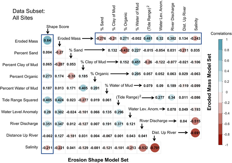
FIGURE 6. Pearson correlation plot results for the All Sites data subset. Upper and lower diagonal plots show correlation values for the Eroded Mass and Erosion Shape model sets, respectively. Correlations with the response variables are boxed in blue.
Two different model sets (Table 3) were used to evaluate the two erodibility response variables identified for this study: 1) eroded mass at τb = 0.2 Pa and 2) the shape of the erosion vs. τb profile as determined by its principal shape component. The goal of the first grouping of explanatory variables (the “Eroded Mass Model Set”) was to determine the relative importance of various sediment properties and hydrodynamic conditions in determining erodibility at a representative, commonly occurring bed stress within the York River. The goal of the second variable grouping (the “Erosion Shape Model Set”) was to determine which sediment and hydrodynamic factors may be important in determining the overall shape of the τc versus eroded mass profile. Explanatory variables that were considered for this second model set were identical to those in the previous model set, but also include eroded mass at 0.2 Pa.
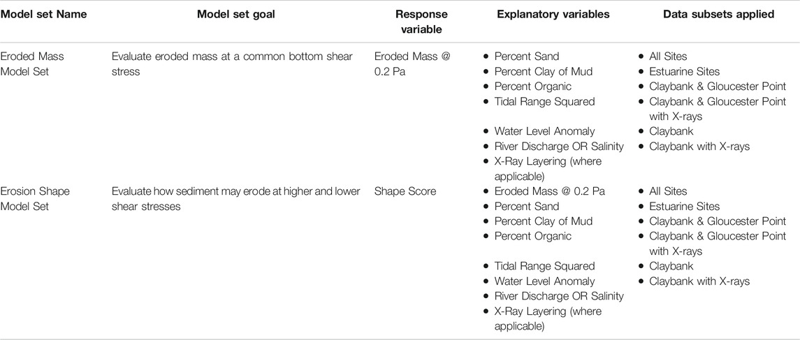
TABLE 3. Model set and data subset framework for multiple linear regression analysis.
Multiple linear regressions were run for each data subset within each model set (see Table 3 for model framework). The general equation for multiple linear regression is:
where y is the predicted response variable, β0 is the model intercept, X1 though Xq represent individual explanatory variables, and β1 through βq represent the corresponding best-fit regression coefficients. Lastly, ϵ is the model residual, i.e., the component of y not reproduced by the other terms on the right-hand-side. Due to the data being standardized prior to model formulation, the absolute value of the β coefficients can be ranked to show which explanatory variables resulted in the largest change in the response variable. For instance, for a β coefficient of 0.3, for every increase of one standard deviation of the explanatory variable, the response variable will increase by 0.3 standard deviations.
All possible combinations of the explanatory variables for each data subset were used in assessing Eq. 3, and the relative likelihood of any given model being the best among the available choices for that data subset was assessed using the Corrected Akaike Information Criterion (AICc). A lower AICc value indicates that a model is more likely to be best, and a model’s ΔAICc value is defined as its own AICc minus that of the model with the lowest AICc value in its model subset. In this study, all models with a ΔAICc value ≤2.0 units are considered comparable models with useful information regarding trends (Burnham and Anderson, 2004). Because ΔAICc values are relative within a given model subset, they cannot be used to compare the explanation of variance of response variables across model subsets. To remedy this, adjusted R2 values were included to describe how much of the data variation was explained by the combination of parameters in each model across sub-model categories.
Application of running means indicated that the average of the past 33 tidal range squared observations (8.5 days—i.e., centered around conditions 4.3 days prior) had the highest correlation with eroded mass at τb = 0.2 Pa. The best correlation between the water level anomaly and eroded mass was found to be over the past 27 cycles (7.0 days). For river discharge, the running average with the highest correlation with eroded mass at 0.2 Pa was over the previous 170 days (i.e., centered around conditions 2.8 months prior).
PCA for Gust profiles was completed to reduce the shape profile containing seven eroded mass values and seven stress values, to one shape score that could be used as a response variable in multiple linear regression. Principal component one (PC1) (i.e., the shape score) explained approximately 83% of the variation of shape within all data subsets (Figure 5D). Positive and negative values of PC1 made the normalized eroded mass profile less and more concave, respectively, than the average profile shape (Figures 5E,F). Negative shape scores corresponded to a geometrically increasing shape profile, such that each increase in stress resulted in a proportionately greater increase in eroded mass. In contrast, positive shape scores tended to indicate a more linear profile or, when most positive, a proportionally smaller increase in eroded mass with each increase in stress. PC1 was the only component whose scores were used as a response variable in the models reported here because PC1 explained ∼83% of the variability in erosion profile shape in all data subsets. PC2 described only ∼11–13% of variation in the erosion profile shapes, and PC3 accounted for just ∼3–4% (Figure 5D).
Initial assessment of relationships among variables was facilitated by correlation plot results (Figure 6) applied to each of the six data subsets listed in Table 1 and Table 3. (The X-ray layering parameter is not part of the All Sites data set in Figure 6 because X-rays were not collected at every site.) A complete set of correlation plot results for all six data subsets are included in Wright et al. (2021).
Despite its dominant role in the erodibility literature (e.g., Mehta, 2014), percent water of mud was consistently found to be poorly or nonsensically correlated with erodibility, and percent water was ultimately dropped from all multiple regression models for all six data subsets. For example, for the All Sites data subset, percent water of mud had the poorest correlation with eroded mass at 0.2 Pa of any variable, with r = −0.002 in the Eroded Mass Model Set (Figure 6). Across the other five data sets, the average magnitude of the correlation between percent water of mud and eroded mass was likewise quite poor, with a mean |r| of 0.111 (Wright et al., 2021). Furthermore, when included in multiple regressions with the other variables, the few models for eroded mass with ΔAICc < 2.0 that retained water content produced a negative β value for percent water (Wright, 2021). This is physically nonsensical given that there is a rich and long-established literature (see Mehta, 2014 and references within) demonstrating that erodibility for fine sediment should be negatively correlated with sediment bulk density (and thus positively correlated with percent water). Possible explanations for the unexpected result for the role of percent water are discussed in Section Limitations Associated With Sampling Approach and Resolution of Bed Properties.
Collinearity among explanatory variables was also assessed using correlation plot results. Among the All Sites explanatory variables that were further considered, salinity had the highest correlations with other variables: namely, with distance upriver (at r = −0.701) and with river discharge (at r = −0.532) within the Erosion Shape Model Set (Figure 6). This is not unexpected, since salinity along the York River estuary is predicted well by a nonlinear model based only on position along the estuary and past river discharge (Parrish et al., 2019). Thus, for the All Sites linear models, salinity was dropped from further consideration. However, for the other data subsets, salinity turned out to be a better predictor of the response variables than river flow, so salinity was utilized in its place. Across all data subsets, which include 452 explanatory variable correlations, only three other cases (not involving river discharge or salinity) had correlation values over 0.6. However, in the individual candidate and global models for those data subsets, vif factors were all below 5.0, so the associated variables were retained.
There were 33 candidate models identified (i.e., models with ΔAICc ≤2.0) within the six data subsets for the Eroded Mass Model Set. Overall, tidal range squared and salinity/river discharge were the most consistent explanatory variables throughout the entire model set, with these variables being retained in 100% of the models in which they were considered. Figure 7A shows average |β| values for each individual data subset, with each subset corresponding to a given bar color. [All individual β and adjusted R2 values for all 33 models are provided in Wright et al. (2021)]. The variables with the highest average |β| values across all of the Eroded Mass Model subsets included past tidal range squared (0.424), salinity (−0.294) / river discharge (0.252), and percent organic (0.226). Variables that were less important, but still had consistent trends in average β were past water level anomaly (0.171), percent sand (−0.143), distance upriver (0.136), percent clay of mud (−0.135), and presence of X-ray layering (0.108).
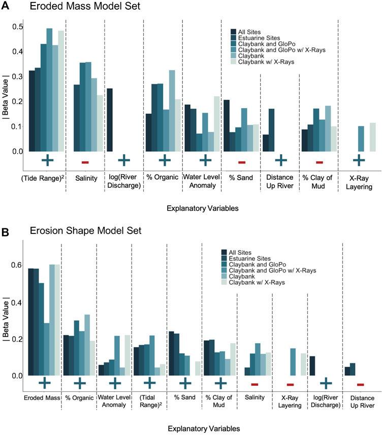
FIGURE 7. Bar graphs showing average absolute β values for each explanatory variable for each data subset (corresponding colors) that were included in candidate models. Signs below bar graphs indicate whether the β value was positive (blue “+” = direct relationship) or negative (red “−” = inverse relationship). Absent lines indicate parameters that were not considered in the model or parameters that were not present in any of the candidate models.
Model performance tended to increase as data subsets became more spatially focused and otherwise specific. Partial residual plots are shown in Figure 8 for representative 5-component models from the All Sites, Claybank & Gloucester Point, and Claybank with X-rays subsets. The slope of the line in each panel is the β value for the corresponding explanatory variable within the model. The β value for the most important explanatory variable (tidal range squared) (Figure 8) increased as the data sets became more localized, and the overall performance of the models with ΔAICc scores of 0 also tended to improve (Appendix Figure A1). As presented in detail in Wright et al. (2021), the multiple All Sites subset models had an average adjusted R2 of 0.392, which increased to an average of 0.464 in the Estuarine Sites subset. Furthermore, both Claybank & Gloucester Point subsets (with and without X-rays) had an average of 0.585, and both Claybank subsets resulted in an average adjusted R2 of 0.609.
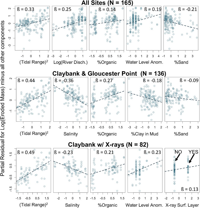
FIGURE 8. Partial residual plots from the Eroded Mass Model Set for three representative, 5-component models from three data subsets. Each plot has standardized units for Xq and for βqXq + ε on the x- and y-axis, respectively. Trend lines each have a slope equal to the parameter’s β value.
The model set for profile shape score consisted of 39 candidate models throughout the six different data subsets. Throughout all data subsets, eroded mass at 0.2 Pa was by far the most prominent explanatory variable for all candidate models, being included in 100% of candidate cases and exhibiting an absolute value for β twice as large as any other variable (Figure 7B, Figure 9). In every model, the relationship between eroded mass and profile shape was positive, such that greater erodibility favored a straighter (or less concave-up) profile (see Figure 5F). Following eroded mass at |β| = 0.519 (averaged across all data sets), the next highest |β| values were for organic proportion at 0.249, water level anomaly at 0.182, tidal range squared at 0.171, and percent sand at 0.166. Six other variables had moderately low average |β| values, ranging between 0.136 and 0.058.
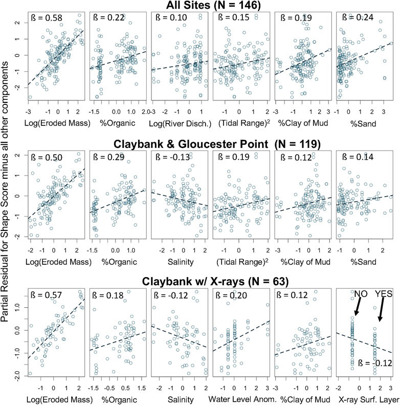
FIGURE 9. As in Figure 8, but from the Erosion Shape Model Set for representative 6-component models.
Given the strong positive relationship between profile shape score and eroded mass at 0.2 Pa, one might initially expect the remaining explanatory variables to show relationships with shape score such that the sign of their β values matched the signs relating them to eroded mass in the previous section. This was indeed the case for percent organic, water level anomaly, tidal range squared, river discharge, and salinity. However, the signs for the β values relating percent sand, percent clay of mud, X-ray layering, and distance upriver to profile shape score were all opposite to signs of the β values relating them to eroded mass.
As was the case for eroded mass at 0.2 Pa, the models for profile shape score also tended to increase in performance as data subsets became more spatially focused, although not as dramatically (Figure 9 and Figure A2). Partial residual plots are shown in Figure 9 for representative 6-component models from the All Sites, Claybank & Gloucester Point, and Claybank with X-rays subsets. The All Sites subset had an averaged adjusted R2 of 0.537, which slightly decreased in the Estuarine Sites subset to 0.517 (see Wright et al., 2021). However, adjusted R2 averages increased again in the Claybank & Gloucester Point subsets and the Claybank subsets to 0.581 and 0.703, respectively.
Using the top-performing (ΔAICc = 0) model from each model subset (Blue circles and blue dashed lines in Appendix Figure A1 and Figure A2), a validation exercise was performed to test the general stability the model fits. Each data subset was split into two halves, with one half used to calibrate new best-fit β values. The new β values were then used to predict the response variable for the validation half (red squares and red dashed lines in Appendix Figure A1 and Figure A2). To help ensure that each half encompassed a similar range of variable values, the calibration half consisted of the first and fourth quarters of each subset in time, and the validation set consisted of the second and third quarters. This was done because the lower- and upper-most estuary had mainly been sampled during the first and second halves of the 15-year time record, respectively.
The adjusted R2 values for the validation data fits were generally similar to the adjusted R2 values for the best model sets (Figure A1 and Figure A2), which demonstrates that the model fits were reasonably stable. In several cases, adjusted R2 was larger for the validation set than the corresponding full data set, indicating that some of the validation data subsets were less noisy than their corresponding full data sets. The regression lines for the validation sets (red dashed lines), however, were almost always somewhat farther from the 1:1 line relative to the full data sets (blue dashed lines), as would be expected.
Two of the explanatory variables with the strongest positive effects on eroded mass at 0.2 Pa across all data subsets highlight the influence of recent physical bed disturbance on bed erodibility. Past tidal range squared, the most influential variable of all, represents the role of recent tidal bed stress in repeatedly suspending and depositing mud, such that the newly disturbed sediment is unconsolidated and easier to subsequently entrain into the water column again. Past water level anomaly, or the absolute difference between observed and predicted tidal range, is interpreted here to represent the role of recent winds causing set-up or set-down of water level, which is also associated with winddriven currents that further physically disturb the seabed, enhancing erodibility.
Several explanatory variables also emphasize that recent deposition increases erodibility as measured by eroded mass at 0.2 Pa. When considering observations from a location that is seaward of the ETM, such as data from Claybank, a decrease in salinity indicates the continued progression of the pool of easily suspended sediment down the estuary and net deposition of mud. Thus, erodibility increases at Claybank as salinity decreases. An increase in percent organic matter in the upper 1 cm of the bed also suggests recent deposition of “fresher,” easier to resuspend muddy flocs. So, erodibility increases with percent organics. Likewise, the presence of layering at the surface as seen by X-radiographs indicates recent deposition, and layering was found to be positively correlated with erodibility. The past water level anomaly may also be associated with recent deposition events in the channels where most of the erodibility measurements were collected. Episodic wind waves associated with the water level anomaly might winnow mud from the shoals, which then might produce temporary deposition and higher erodibility in the neighboring channels.
Multiple explanatory variables highlight the role of time since deposition (i.e., consolidation time), the effect of erosion exposing older sediment, and/or the past winnowing of fines decreasing eroded mass at 0.2 Pa. At a given site below the ETM, an increase in salinity indicates the likely net movement of mud upstream and away from the site, exposing older sediment and decreasing erodibility. As “fresher” mud migrates away, one would expect lower percent organics and higher percent sand, trends which are each seen to be associated with reduced erodibility in all models in which they appear. Likewise, the negative association between mottled X-radiographs and eroded mass at 0.2 Pa indicates that older sediment (i.e., that which has had time to be fully bioturbated) is less erodible. A lower fraction of silts (as indicated by a higher clay fraction of mud and/or higher sand fraction overall) is associated with lower erodibility in the York. As previously recognized by many investigators, fine sediments tend to become harder to erode as their clay-sized grain content increases because of an increase in grain-to-grain cohesion as grains become smaller (e.g., Postma, 1967; Dade et al., 1992; Roberts et al., 1998; Mehta, 2014). In contrast, mixtures containing sand-sized sediments eventually become harder to erode as their sand content increases, because suspension of non-cohesive sediment is more difficult as grain size increases.
An important finding in this study with regards to consolidation of the uppermost seabed is that the strong increase in erodibility due to recent physical disturbance (as parameterized by tidal range squared and water level anomaly) only lasts several days. For both tidal range squared and water level anomaly, the average of the previous ∼7 to 8 days of observations—i.e., a time period centered around conditions ∼4 days prior—had the highest correlation with eroded mass at 0.2 Pa. This timescale of a few days is consistent with consolidation times scales reported for high water content muds in laboratory studies (Mehta, 2014 and references within), with those found to work well in modeling studies (Rinehimer et al., 2008; Sanford, 2008; Sherwood et al., 2018), and is also close to the time scale for the transition from spring to neap tides (as likewise noted by Mehta, 2014). Similar results have also been seen in the field by others. Based on a weekly time-series of five cores from the York River estuary, Kraatz (2013) previously found that eroded mass at 0.2 Pa was best correlated to the tidal range averaged over the previous 5 days, and Huang et al. (2020) found that it took approximately 7 days for sediment layers to consolidate after being deposited by tides in the Pearl River Estuary.
Throughout the Eroded Mass Model Set, the hydrodynamic explanatory variables had a statistically stronger relationship to eroded mass at 0.2 Pa than did the sediment property variables, according to average |β| values. However, hydrodynamic variables influence erodibility indirectly. Physically, erodibility is associated more directly with the properties of the bed, as seen in laboratory consolidation and erosion experiments focusing on specific sediment grain sizes and bulk densities (Roberts et al., 1998; Mehta, 2014). Nonetheless, for the Eroded Mass Model Set, the parameter with the highest average |β| value was past tidal range squared (0.424; Figure 7A). Past tidal range squared was present in all candidate models, and it had the highest |β| within all 33 cases. The mechanistically similar parameter of past water level anomaly was also present in every subset of models. These two hydrodynamic parameters, which are interpreted as proxies for physical bed disturbance and reduced consolidation, predicted erodibility more successfully than most directly measured sediment properties. The second most important variable of all, salinity at an average |β| of 0.294, is also a hydrodynamic variable, as is river discharge at third most important (average |β| = 0.226).
The overall importance of hydrodynamic variables may have ramifications for enhanced performance of bed erodibility routines within computationally-intensive, multiparameter numerical models, such as 3D hydrodynamic codes that include biogeochemistry. It is easier to accurately model hydrodynamic environmental variables than to reproduce centimeter or millimeter-scale sediment bed properties. By applying these empirical relationships between hydrodynamics and erodibility in the York or by developing similar relationships for other estuaries, modelers may be able to produce a more accurate representation of sediment bed critical stresses and associated eroded mass in given areas of an estuary by only having to include the effects of external variables such as recent velocities (or bed stresses), salinity, and/or river discharge. These parameters are likely more straightforward to model than having to precisely reproduce sediment properties throughout the estuary, especially when they are spatially heterogeneous. If it is possible to represent bed grain size and organic matter well in the estuarine numerical model, a multiple regression to predict erodibility could also use these variables to further improve erodibility results.
The Erosion Shape Model Set included an additional sediment property, namely eroded mass at 0.2 Pa, as an explanatory variable, which ended up having the largest influence on shape score by far. Eroded mass at 0.2 Pa had the highest average |β| in all the candidate models across all Erosion Shape Model subsets, with an average of 0.519 which was more than twice as large as |β| for the next most important erosion shape variable (Figure 7B). Higher eroded mass at 0.2 Pa tended to make the shape score more positive, which indicated a more linear eroded mass profile (blue PC1 > SD lines in Figures 5E,F). Conversely, beds with low erodibility tended to have a more strongly curved, concave-upward relationship between applied stress and total eroded mass (red PC1 < -SD lines in Figures 5E,F). Although they did not comment on this shape trend, Dickhudt et al. (2009) also observed more strongly curved profiles at low stress and an increase in profile linearity at higher erodibility. Dickhudt et al. (2009) fit a curve of the form τc ∼ mb plus an offset to groupings of their York River erodibility profiles, where m is cumulative eroded mass. Values of b closer to 1 indicate a more strongly linear fit, whereas smaller b indicates a more concave fit. For their “low,” “transitional,” and “high” erodibility groups, Dickhudt et al. (2009) found b = 0.51, 0.65, and 0.75, respectively. An analogous fit to the lower erodibility (red), intermediate (black), and higher erodibility (blue) curves from the present study (Figure 5F) yields b = 0.29, 0.60, and 0.89, which is a consistent trend.
The low erodibility, concave-upward shape may represent a near-steady-state erodibility profile present in the absence of significant recent bed disturbance, such as immediately following neap tide. This shape is similar to the concave equilibrium eroded mass vs. applied stress profile assumed by modelers of muddy bed erodibility in the absence of disturbance (Rinehimer et al., 2008; Sanford, 2008; Sherwood et al., 2018). The transition towards a more linear erodibility profile in the presence of more frequent recent disturbance (and higher overall erodibility), such as immediately following spring tide, reflects a relatively larger increase in incremental eroded mass in the range of ∼0.2 to 0.4 Pa than at higher or lower applied stress (Figure 5F). This makes sense, since the frequency at which the τb = 0.2 to 0.4 Pa is reached in the York notably increases during spring tides (see Figure 3B). Stresses larger than 0.4 Pa are not reached very often, even on spring tides, and stresses less than 0.2 Pa are reached on nearly every tide, so spring-neap variability in bed disturbance does not change erodibility as dramatically at either of these τb end members.
Similar to the magnitude of erodibility, the erosion shape profile can potentially be predicted by numerical models in some cases based solely on hydrodynamic forcings. As discussed in Section Hydrodynamics Can Serve as a Proxy for Effects of Bed Properties on Erodibility, eroded mass for very muddy beds can be predicted relatively well based on recent hydrodynamic conditions. In turn, eroded mass is the most influential predictor of erosion shape, with |β| values twice that of any other explanatory variable. Thus, modelers can constrain both the magnitude and profile shape of the critical stress in very muddy sediments by focusing largely on the hydrodynamic history of a study area. In this respect, the findings of this study are highly consistent with the conceptual approach of Sanford (2008), who included a mud-only case for which changes in erodibility in time were predicted based only on a time history of tidally varying applied bed stress.
This study was largely an opportunistic analysis of an extensive sediment erodibility data set that was not collected for a single purpose. The samples were collected over 15 years at differing temporal and spatial scales for various projects. Due to clustered sampling in time and space associated with the past measurements, many standard statistical assumptions were not well adhered to. Thus, formal statistical significance levels such as p-values were not reported here for any of the multiple linear regressions. Over 75% of the samples used in this study were taken during the spring and summer months (March through August). Therefore, it is hard to definitively state that explanatory variables with seasonal changes like discharge, salinity, and water level anomaly follow the same predictive models all year round. For example, the average wind speed and freshwater discharge along the York are greater in winter than in summer by a factor of ∼1.3 and ∼3.2, respectively. Additionally, the data set was heavily skewed by the Claybank location, with over 65% of samples being in that subset. Given these sampling design limitations, the goal here was not to rigorously focus on the absolute level of the statistical significance of the results. Rather, the focus was on trends in the responses and the relative importance of one explanatory variable versus another.
In addition, the field methodology for subsampling sediment cores for water content analysis most likely did not sufficiently resolve the very surface of the sediment core. Based on a mean water content of 75.5% (Table 2), the upper 1 mm of the seabed contained, on average, 0.29 kg/m2 of dry sediment. The average dry sediment mass eroded at 0.2 Pa was only 0.089 kg/m2 (Table 2), and >90% of cases eroded less than 0.29 kg/m2 (Wright et al., 2021). Thus, the Gust experiments, on average, eroded only ∼0.3 mm into the bed at 0.2 Pa, and >90% of Gust experiments eroded less than 1 mm at 0.2 Pa. Unfortunately, subsamples from box cores did not attempt to resolve the uppermost 1 mm, and instead the top 1 cm from sub-cores was homogenized. Quite possibly, the water content of the full 1 cm of the upper seabed was not sensibly correlated to the water content of the uppermost 0.3 to 1 mm. The same methodology was used in the Dickhudt et al. (2009, 2011) studies, and it may be a contributing factor to why they also found no meaningful relationships between the variation of water content of mud in the York River estuary and sediment erodibility. In contrast, sensible and meaningful correlations with eroded mass at 0.2 Pa were found for the clay content of mud, sand content, and organic content of the top 1 cm. A logical explanation is that vertical gradients in clay, sand, and organic content over the top 1 cm are not nearly as strong as the vertical gradients in water content.
There may be additional factors relevant to moderately turbid, muddy tidal estuaries like the York that could make the correlation between water content over the top 1 cm and erodibility noisier than that observed in well-controlled lab experiments. As also noted by Dickhudt et al. (2009), the water content of mud over the top 1 cm in the York varies much less than other potential controls on erodibility. The standard deviation of water content divided by its mean was only 0.06 (Table 2). This means that even modest errors in quantifying water content could overwhelm the signal in the variance. In contrast, standard deviations divided by the mean for the bed properties with the most observed influence on erodibility, namely organic content and sand content, were 0.55 and 1.1, respectively, meaning that their signals were more likely to exceed their noise. Another complication when averaging over the top 1 cm may be that water content at this scale is positively correlated to percent clay of mud (Figure 6), possibly because high clay content reduces mud permeability (Zhang et al., 2015). Clay content of mud, in turn, was found to reduce erodibility. So, given the relatively small variation in water content in York River mud when averaged over the top cm of the bed, variations in clay content may at least partly counteract the influence of the mud’s water content.
There are variables that were not included in this analysis that could also influence sediment erodibility and produce some of the unexplained variance remaining in the models. These include local mean water depth, position across the channel, and bedform types. Mean water depth and across-channel position were considered but were not found to notably account for variance in erodibility in this study’s data set within the context of general linear models. This may be because so much of the data in this study were repeatedly collected at a few specific sites with relatively little sample-to-sample variation in depth or lateral location. Bedform types were not used because of a lack of observations corresponding with each sample, although mud furrows have been shown to potentially play a role in physical disturbance of the bed in the York River estuary (Dellapenna et al., 1998, 2003). In general, additional explanatory variables were not available because this data set dates back to 2005. The variables used in the final model formulations are either those that were collected according to lab protocol and have stayed consistent from 2005 to 2019 or ones that were accessible from online sources for each of the sediment cores. For example, the smaller number of pellet abundance samples (58 samples) versus most other bed properties (165 samples) stems in part from it not becoming a standard variable until later in the sampling record.
Within estuaries characterized by a main channel bordered by distinct shoals, such as the York River, lateral changes in sediment properties and hydrodynamic properties may especially influence sediment bed erodibility. The northeast and the southwest shoals of the York River tend to differ in terms of grain-size distribution and the mechanisms of sediment reworking (Hinchey, 2002; Dellapenna et al., 2003; Kniskern and Kuehl, 2003). For example, the northeast shoal of the river is sandier than the southwest shoal. Ideally, the inclusion of grain-size distribution and distance upriver might be able to adequately account for these observed differences. However, Huzzey (1988) reported lateral density gradients at Claybank, with homogenous lateral densities only present during maximum tidal currents. Huzzey (1988) also states that the cross-estuarine gradients could drive significant lateral water circulation in the area, which may likely be strong enough to preferentially erode sediment and deposit in different areas of a channel cross-section, especially in such a soft-bottomed area such as Claybank. The influence of lateral circulation and resulting changes in lateral transport convergence and erodibility have been suggested for the neighboring James River Estuary (Huijts et al., 2006). In the current study, only longitudinal estuary circulation was considered in the form of river discharge and salinity affecting the presence of the estuarine turbidity maxima.
Only linear relationships were reported here, but non-linear relationships were also considered during early stages of the analysis. Generalized additive models (GAMs) were initially included, but they tended to show exaggerated, oscillatory, and unrealistically non-linear relationships with many of the explanatory variables due to overfitting. When this tendency was compensated for by increased smoothing in the GAM settings, the results then provided insights very similar to multiple linear regression, suggesting that the added complexity of GAMs was not warranted. Nonetheless, at least one potential explanatory variable, namely resilient fecal pellets, seemed to have a systematically non-linear relationship with erodibility (Figure 10). In the pellet subset, there was an initial increase in eroded mass with pellet abundance at a low proportion of pellets, but then eroded mass began to decrease again at a higher proportion of pellets. Perhaps the initial increase in pellet abundance is acting as a proxy for decreasing clay content of mud, which would increase erodibility. Eventually, continued increases in pellet abundance may be a proxy for behavior similar to coarser non-cohesive sediment, such as sand, which would decrease erodibility once more. It could be beneficial to better explore these non-linear relationships in further investigations of this or other similar datasets.
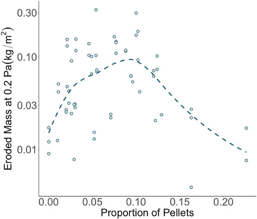
FIGURE 10. Eroded mass at 0.2 Pa versus the proportion of total sediment mass composed of resilient pellets for the top centimeter of all cores sampled for pellets. A superimposed smoother highlights the possibility of a non-linear relationship between eroded mass and pellet proportion.
The current study would have likely explained a greater amount of variance within the dataset had it included more accurate measurements for water content in the upper few mm of the seabed. The upper few mm of very soft muddy sediments, like those found in the York River estuary, can be difficult to sample. Perhaps higher resolution methodologies for measuring water content, such as resistivity profiling (Wheatcroft and Borgeld, 2000), fiber optical backscatter profiling (Hooshmand et al., 2015), or freeze coring followed by thin slicing (Harrison et al., 2016) could be used in conjunction with future sediment sampling to better determine the true fine-scale influence of this parameter on sediment erodibility.
Finally, future statistical studies of controls on bed erodibility in muddy estuaries would also benefit from improved field sampling in terms of experimental design. Choices for future erodibility coring sites should utilize aspects of random sampling in time and space to reduce potential autocorrelation of samples and better ensure that the true range of variability in explanatory and response variables is well represented. Nonetheless, the large sample size and temporal duration of the present data set still makes it a uniquely valuable resource for better understanding controls on estuarine sediment bed erodibility, as long as its inherent limitations are recognized.
Multiple linear regressions were applied to an extensive, 15-year data set from the York River estuary to determine and better understand which sediment and hydrodynamic properties are most important in controlling estuarine bed erodibility in terms of 1) the magnitude of eroded mass at a characteristic bed stress (0.2 Pa), also termed “eroded mass” and 2) the normalized shape of the eroded mass profile between 0 and 0.56 Pa, also termed “erosion shape.” Major conclusions from the study include:
• The explanatory variables in the Eroded Mass Model Set (past tide range squared, salinity, percent organic, past water level anomaly, past river discharge, percent sand, percent clay of mud, and distance upriver) supported the roles of 1) recent deposition and bed disturbance increasing erodibility and 2) cohesion/consolidation and erosion/winnowing of fines decreasing erodibility. Trends regarding the effects of explanatory variables were highly consistent across multiple models.
• The Eroded Mass Model Set resulted in larger magnitude regression coefficients for hydrodynamic properties than for sediment properties, indicating that hydrodynamics can serve as a proxy for the effect of consolidation state on erodibility. Past increases in tidal range squared and water level anomaly are related to previous disturbance of the surface sediment layers and likely create a less stable, more erodible sediment surface. Seaward of the turbidity maximum, lower salinity/higher discharge are related to new deposition, which also drives higher erodibility. The best-fit ∼7 to 8 days lag for the effects of tidal range squared and water level anomaly identifies a characteristic time-scale for mud consolidation that is close to the period between spring and neap tide.
• The response of the Erosion Shape Model Set was dominated by the effect of eroded mass on the shape of the eroded mass profile, such that a strongly concave profile shape under low erodibility conditions became substantially more linear as erodibility increased. The low erodibility, strongly curved shape may represent a near-steady-state erodibility profile present in the absence of significant recent bed disturbance, such as immediately after neap tide. The transition towards a more linear erodibility profile in the presence of more frequent recent disturbance, such as immediately following spring tide, reflects a relatively larger increase in incremental eroded mass in the mid-to-upper-mid range of periodically observed bed stresses.
• The results of this study suggest that numerical modelers may be able to use their simulations of hydrodynamic variables in very muddy estuarine systems as a proxy for consolidation state to help predict the magnitude and shape of the eroded mass versus critical stress profile, rather than relying solely on predicted sediment bed properties. Some muddy sediment properties, like bulk density and clay content of mud can be difficult to model, especially where they are spatially and temporally heterogeneous. Parameters like past river discharge, salinity, and recent velocities (or bed stresses) are often much more accessible.
• Although many of the variables were adequately described with linear relationships, some may be better represented with non-linear modeling. Also, future sampling would benefit from higher resolution measurements of water content within the upper few millimeters of the seabed. Finally, improved distribution of spatial and temporal sampling would likely enhance understanding and prediction of erodibility across the entire estuarine system.
The datasets presented in this study can be found in online repositories. The names of the repository/repositories and accession number(s) can be found below: William & Mary ScholarWorks https://doi.org/10.25773/nm2b-hy57.
All authors played an essential role in designing this project. In addition, CW completed formal analysis and wrote the original draft manuscript as part of her master’s thesis; CF provided critical feedback in reviewing and editing the manuscript; and GM played a key role in overseeing field data collection and laboratory analysis.
This work was funded by the Virginia Institute of Marine Science, SERDP Projects MR-2409, MR18-1233, and MR-1265, and NSF Awards OCE-0536572, OCE-1061781, and OCE-1459708.
The authors declare that the research was conducted in the absence of any commercial or financial relationships that could be construed as a potential conflict of interest.
All claims expressed in this article are solely those of the authors and do not necessarily represent those of their affiliated organizations, or those of the publisher, the editors and the reviewers. Any product that may be evaluated in this article, or claim that may be made by its manufacturer, is not guaranteed or endorsed by the publisher.
The authors would like to thank all past members of the Coastal Hydrodynamics and Sediment Dynamics lab that had a hand in collecting and/or processing these data, with special thanks to P. Dickhudt, K. Fall, and L. Kraatz. C. Harris, L. Schaffner, and N. Stark provided helpful comments on an early version of this manuscript, and three Frontiers reviewers provided especially insightful suggestions for improvement. This is contribution 4068 of the Virginia Institute of Marine Science, William & Mary.
Andersen, T. J. (2001). Seasonal Variation in Erodibility of Two Temperate, Microtidal Mudflats. Estuarine, Coastal Shelf Sci. 53, 1–12. doi:10.1006/ecss.2001.0790
Barry, K. M., Thieke, R. J., and Mehta, A. J. (2006). Quasi-hydrodynamic Lubrication Effect of Clay Particles on Sand Grain Erosion. Estuarine, Coastal Shelf Sci. 67, 161–169. doi:10.1016/j.ecss.2005.11.009
Bearman, J. A., Friedrichs, C. T., Jaffe, B. E., and Foxgrover, A. C. (2010). Spatial Trends in Tidal Flat Shape and Associated Environmental Parameters in South San Francisco Bay. J. Coastal Res. 262, 342–349. doi:10.2112/08-1094.1
Bilici, C., Stark, N., Friedrichs, C. T., and Massey, G. M. (2019). Coupled Sedimentological and Geotechnical Data Analysis of Surficial Sediment Layer Characteristics in a Tidal Estuary. Geo-Mar. Lett. 39, 175–189. doi:10.1007/s00367-019-00565-3
Brouwer, R. L., Schramkowski, G. P., Dijkstra, Y. M., and Schuttelaars, H. M. (2018). Time Evolution of Estuarine Turbidity Maxima in Well-Mixed, Tidally Dominated Estuaries: The Role of Availability- and Erosion-Limited Conditions. J. Phys. Oceanogr 48, 1629–1650. doi:10.1175/JPO-D-17-0183.1
Burchard, H., Schuttelaars, H. M., and Ralston, D. K. (2018). Sediment Trapping in Estuaries. Annu. Rev. Mar. Sci. 10, 371–395. doi:10.1146/annurev-marine-010816-060535
Burnham, K., and Anderson, D. (2004). Model Selection and Multi-Model Inference. Second. New York: Springer-Verlag.
Cartwright, G. M., Friedrichs, C. T., Dickhudt, P. J., Gass, T., and Farmer, F. H. (2009). Using the Acoustic Doppler Velocimeter (ADV) in the MUDBED Real-Time Observing System. OCEANS 2009. New York: Institute of Electrical and Electronics Engineers, 642–655. doi:10.23919/OCEANS.2009.5422146
Cloern, J. E. (1987). Turbidity as a Control on Phytoplankton Biomass and Productivity in Estuaries. Continental Shelf Res. 7, 1367–1381. doi:10.1016/0278-4343(87)90042-2
Cooper, N., and Cooke, S. (2018). “Risky Business: Dealing with Unexploded Ordnance (UXO) in the marine Environment,” in Coasts, Marine Structures and Breakwaters 2017. Editor K. Burgess (London: Institution of Civil Engineers), 157–167. doi:10.1680/cmsb.63174.0157
Cozzoli, F., Gjoni, V., Del Pasqua, M., Hu, Z., Ysebaert, T., Herman, P. M. J., et al. (2019). A Process Based Model of Cohesive Sediment Resuspension under Bioturbators' Influence. Sci. Total Environ. 670, 18–30. doi:10.1016/j.scitotenv.2019.03.085
Dade, W. B., Nowell, A. R. M., and Jumars, P. A. (1992). Predicting Erosion Resistance of Muds. Mar. Geology. 105, 285–297. doi:10.1016/0025-3227(92)90194-M
Dellapenna, T. M., Kuehl, S. A., and Schaffner, L. C. (2003). Ephemeral Deposition, Seabed Mixing and fine-scale Strata Formation in the York River Estuary, Chesapeake Bay. Estuarine, Coastal Shelf Sci. 58, 621–643. doi:10.1016/S0272-7714(03)00174-4
Dellapenna, T. M., Kuehl, S. A., and Schaffner, L. C. (1998). Sea-bed Mixing and Particle Residence Times in Biologically and Physically Dominated Estuarine Systems: a Comparison of Lower Chesapeake Bay and the York River Subestuary. Estuarine, Coastal Shelf Sci. 46, 777–795. doi:10.1006/ecss.1997.0316
Dickhudt, P. J., Friedrichs, C. T., and Sanford, L. P. (2011). Mud Matrix Solids Fraction and Bed Erodibility in the York River Estuary, USA, and Other Muddy Environments. Continental Shelf Res. 31, S3–S13. doi:10.1016/j.csr.2010.02.008
Dickhudt, P. J., Friedrichs, C. T., Schaffner, L. C., and Sanford, L. P. (2009). Spatial and Temporal Variation in Cohesive Sediment Erodibility in the York River Estuary, Eastern USA: A Biologically Influenced Equilibrium Modified by Seasonal Deposition. Mar. Geology. 267, 128–140. doi:10.1016/j.margeo.2009.09.009
Fall, K. A. (2012). Relationships Among Fine Sediment Settling and Suspension, Bed Erodibility, and Particle Type in the York River Estuary, Virginia. Master’s Thesis. William & Mary. doi:10.25773/v5-hfz9-5r79
Fall, K. A., Harris, C. K., Friedrichs, C. T., Rinehimer, J. P., and Sherwood, C. R. (2014). Model Behavior and Sensitivity in an Application of the Cohesive Bed Component of the Community Sediment Transport Modeling System for the York River Estuary, VA. J. Mar. Sci. Eng. 2, 413–436. doi:10.3390/jmse2020413
Fall, K. A. (2020). Influence of Suspended Particle Size and Composition on Particle Image Processing, Estuarine Floc Fractal Properties, and Resulting Estuarine Light Attenuation. Dissertation. William & Mary. doi:10.25773/v5-nn75-t992
Friedrichs, C., Cartwright, G., and Dickhudt, P. (2008). Quantifying Benthic Exchange of fine Sediment via Continuous, Noninvasive Measurements of Settling Velocity and Bed Erodibility. Oceanog. 21, 168–172. doi:10.5670/oceanog.2008.14
Friedrichs, C. T. (1995). Stability Shear Stress and Equilibrium Cross-Sectional Geometry of Sheltered Tidal Channels. J. Coast. Res. 11, 1062–1074. https://www.jstor.org/stable/4298411.
Friedrichs, C. T., Armbrust, B. A., and de Swart, H. E. (1998). Hydrodynamics and Equilibrium Sediment Dynamics of Shallow, Funnel-Shaped Tidal Estuaries. Physics of Estuaries and Coastal Seas. Editors J. Dronkers, and M. Scheffers (Rotterdam: A.A. Balkema), 315–328.
Friedrichs, C. T. (2009). York River Physical Oceanography and Sediment Transport. J. Coastal Res. SI 57, 17–22. doi:10.2112/1551-5036-57.sp1.17
Friedrichs, C. T. (2010). Barotropic Tides in Channelized Estuaries. Contemporary Issues in Estuarine Physics. Editors A. Valle-Levinson (Cambridge: Cambridge University Press), 27–61. doi:10.1017/CBO9780511676567.004
Gillett, D. J., and Schaffner, L. C. (2009). Benthos of the York River. J. Coastal Res. 10057, 80–98. doi:10.2112/1551-5036-57.sp1.80
Grabowski, R. C., Droppo, I. G., and Wharton, G. (2011). Erodibility of Cohesive Sediment: The Importance of Sediment Properties. Earth-Science Rev. 105, 101–120. doi:10.1016/j.earscirev.2011.01.008
Gust, G., and Müller, V. (1997). Interfacial Hydrodynamics and Entrainment Functions of Currently Used Erosion Devices. Cohesive Sediments. Editors N. Burt, R. Parker, and J. Watts (New York: Wiley), 149–174.
Harrison, B. K., Myrbo, A., Flood, B. E., and Bailey, J. V. (2016). Identification of Subannual Patterns in Microbial Community Signatures from Individual Sedimentary Laminae Using a Freeze-Coring Approach. Limnol. Oceanogr 61, 735–747. doi:10.1002/lno.10250
Haven, D. S., and Morales-Alamo, R. (1968). Occurrence and Transport of Faecal Pellets in Suspension in a Tidal Estuary. Sediment. Geology. 2, 141–151. doi:10.1016/0037-0738(68)90033-X
Hinchey, E. K. (2002). Organism-Sediment Interactions: The Role of Seabed Dynamics in Structuring the Mesohaline York River Macrobenthic Community. Dissertation. William & Mary. doi:10.25773/v5-qt91bm43
Hooshmand, A., Horner‐Devine, A. R., and Lamb, M. P. (2015). Structure of Turbulence and Sediment Stratification in Wave‐supported Mud Layers. J. Geophys. Res. Oceans 120, 2430–2448. doi:10.1002/2014JC010231
Huang, W., Zhang, H., Zhu, L., Chen, L., Zhang, G., Gong, W., et al. (2020). In-situ Study of the Spatiotemporal Variability of Sediment Erodibility in a Microtidal Estuary. Estuarine, Coastal Shelf Sci. 232, 106530. doi:10.1016/j.ecss.2019.106530
Huijts, K. M. H., Schuttelaars, H. M., De Swart, H. E., and Valle-Levinson, A. (2006). Lateral Entrapment of Sediment in Tidal Estuaries: An Idealized Model Study. J. Geophys. Res. 111, C12. doi:10.1029/2006JC003615
Huzzey, L. M. (1988). The Lateral Density Distribution in a Partially Mixed Estuary. Estuarine, Coastal Shelf Sci. 26, 351–358. doi:10.1016/0272-7714(88)90017-0
Iddrisu, W. A., Nokoe, K. S., Luguterah, A., and Antwi, E. O. (2017). Generalized Additive Mixed Modelling of River Discharge in the Black Volta River. Ojs 07, 621–632. doi:10.4236/ojs.2017.74043
Jacobs, W., Le Hir, P., Van Kesteren, W., and Cann, P. (2011). Erosion Threshold of Sand-Mud Mixtures. Continental Shelf Res. 31, S14–S25. doi:10.1016/j.csr.2010.05.012
James, G., Witten, D., Hastie, T., and Tibshirani, R. (2013). An Introduction to Statistical Learning. New York: Springer.
Jepsen, R., Roberts, J., and Lick, W. (1997). Effects of Bulk Density on Sediment Erosion Rates. Water Air Soil Pollut. 99, 21–31. doi:10.1007/bf02406841
Kim, S. C., Friedrichs, C. T., Maa, J. Y., and Wright, L. D. (2000). Estimating Bottom Stress in Tidal Boundary Layer from Acoustic Doppler Velocimeter Data. J. Hydraul. Eng. 126, 6. doi:10.1061/(asce)0733-9429(2000)126:6(399)
Kniskern, T. A., and Kuehl, S. A. (2003). Spatial and Temporal Variability of Seabed Disturbance in the York River Subestuary. Estuarine, Coastal Shelf Sci. 58, 37–55. doi:10.1016/S0272-7714(03)00052-0
Kraatz, L. M. (2013). Acoustic and Sedimentological Investigations of Seabed Conditions and Related Biogeological Parameters in a Tidally Energetic, Fine-grained Environment. Dissertation. William & Mary, Virginia: York River Estuary. doi:10.25773/v5-cq0w-8d39
Kruk, C., Martínez, A., Nogueira, L., Alonso, C., and Calliari, D. (2015). Morphological Traits Variability Reflects Light Limitation of Phytoplankton Production in a Highly Productive Subtropical Estuary (Río de la Plata, South America). Mar. Biol. 162, 331–341. doi:10.1007/s00227-014-2568-6
Lanzoni, S., and Seminara, G. (2002). Long-term Evolution and Morphodynamic Equilibrium of Tidal Channels. J. Geophys. Res. Oceans 107, C1. doi:10.1029/2000JC000468
Li, B., Cozzoli, F., Soissons, L. M., Bouma, T. J., and Chen, L. (2017). Effects of Bioturbation on the Erodibility of Cohesive versus Non-cohesive Sediments along a Current-Velocity Gradient: A Case Study on Cockles. J. Exp. Mar. Biol. Ecol. 496, 84–90. doi:10.1016/j.jembe.2017.08.002
Lin, J., and Kuo, A. Y. (2001). Secondary Turbidity Maximum in a Partially Mixed Microtidal Estuary. Estuaries, 24, 707–720. doi:10.2307/1352879
Lucas, C. H., Widdows, J., and Wall, L. (2003). Relating Spatial and Temporal Variability in Sediment Chlorophylla and Carbohydrate Distribution with Erodibility of a Tidal Flat. Estuaries 26, 885–893. doi:10.1007/BF02803347
Luckenbach, M. W. (1986). Sediment Stability Around Animal Tubes: The Roles of Hydrodynamic Processes and Biotic Activity. Limnol. Oceanogr. 31, 779–787. doi:10.4319/lo.1986.31.4.0779
Massey, G. M., Wright, C. L., Friedrichs, C. T., Stark, N., and Kiptoo, D. (2019). York River Estuary Data in Support of: Improved Penetrometer Performance in Stratified Sediment for Cost-Effective Characterization, Monitoring and Management of Submerged Munitions Sites. Report. Va. Inst. Mar. Sci. William & Mary. doi:10.25773/2rze-fg21
Mehta, A. (2014). An Introduction to Hydraulics of Fine Sediment Transport. New Jersey: World Scientific.
Moore, K. A., Wetzel, R. L., and Orth, R. J. (1997). Seasonal Pulses of Turbidity and Their Relations to Eelgrass (Zostera marina L.) Survival in an Estuary. J. Exp. Mar. Biol. Ecol. 215, 115–134. doi:10.1016/s0022-0981(96)02774-8
Moriarty, J. M., Friedrichs, M. A., and Harris, C. K. (2021). Seabed Resuspension in the Chesapeake Bay Implications for Biogeochemical Cycling and Hypoxia. Estuaries Coasts 44, 103–122. doi:10.1007/s12237-020-00763-8
National Oceanic and Atmospheric Administration (2021). Tides and Currents for Yorktown USCG VA. Access: https://tidesandcurrents.noaa.gov/waterlevels.html?id=8637689.
Nichols, M. M., Kim, S. C., and Brouwer, C. M. (1991). Sediment Characterization of Coastal Lagoons and Bays, Virginian Province. Report. Va. Inst. Mar. Sci. William & Mary. doi:10.21220/V5BQ60
Olabarrieta, M., Geyer, W. R., Coco, G., Friedrichs, C. T., and Cao, Z. (2018). Effects of Density‐Driven Flows on the Long‐Term Morphodynamic Evolution of Funnel‐Shaped Estuaries. J. Geophys. Res. Earth Surf. 123, 2901–2924. doi:10.1029/2017JF004527
Parrish, D., Reay, W., Shields, E., and Friedrichs, C. (2019). “Investigation of an Historic Low Salinity Event in the York River Estuary, Chesapeake Bay,” in 25th Biennial Conference of the Coastal and Estuarine Research Federation, 3–7. https://cerf.confex.com/cerf/2019/meetingapp.cgi/Paper/6256.
Postma, H. (1967). Sediment Transport and Sedimentation in the Estuarine environment. Estuaries. Editor G. H. Lauff (Washington, DC: American Association for the Advancement of Science), 158–179.
Reay, W. G. (2009). Water Quality within the York River Estuary. J. Coastal Res. SI 57, 23–39. doi:10.2112/1551-5036-57.sp1.23
Rinehimer, J. P., Harris, C. K., Sherwood, C. R., and Sanford, L. P. (2008). Estimating Cohesive Sediment Erosion and Consolidation in a Muddy, Tidally-Dominated Environment: Model Behavior and Sensitivity. Estuarine and Coastal Modeling (2007). Editor M. L. Spaulding (Reston, VA: American Society of Civil Engineers), 819–838. doi:10.1061/40990(324)44
Roberts, J., Jepsen, R., Gotthard, D., and Lick, W. (1998). Effects of Particle Size and Bulk Density on Erosion of Quartz Particles. J. Hydraul. Eng. 124, 12. doi:10.1061/(asce)0733-9429(1998)124:12(1261)
Sanford, L. P., and Maa, J. P. Y. (2001). A Unified Erosion Formulation for fine Sediments. Mar. Geol. 179. doi:10.1016/s0025-3227(01)00201-8
Sanford, L. P. (2008). Modeling a Dynamically Varying Mixed Sediment Bed with Erosion, Deposition, Bioturbation, Consolidation, and Armoring. Comput. Geosciences 34, 1263–1283. doi:10.1016/j.cageo.2008.02.011
Schaffner, L. C., Hinchey, E. K., Dellapenna, T. M., Friedrichs, C. T., Neubauer, M. E., Smith, M. E., et al. (2001). “Physical Energy Regimes, Sea-Bed Dynamics and Organism-Sediment Interactions along an Estuarine Gradient,” in Organism–sediment Interactions. Editors J. Y. Aller, S. A. Woodin, and R. C. Aller (Columbia, SC: University of South Carolina Press), 161–182.
Scully, M. E., Friedrichs, C., and Brubaker, J. (2005). Control of Estuarine Stratification and Mixing by Wind-Induced Straining of the Estuarine Density Field. Estuaries 28, 321–326. doi:10.1007/BF02693915
Sherwood, C. R., Aretxabaleta, A. L., Harris, C. K., Rinehimer, J. P., Verney, R., and Ferré, B. (2018). Cohesive and Mixed Sediment in the Regional Ocean Modeling System (ROMS v3.6) Implemented in the Coupled Ocean-Atmosphere-Wave-Sediment Transport Modeling System (COAWST R1234). Geosci. Model. Dev. 11, 1849–1871. doi:10.5194/gmd-11-1849-2018
Sin, Y., Wetzel, R. L., and Anderson, I. C. (1999). Spatial and Temporal Characteristics of Nutrient and Phytoplankton Dynamics in the York River Estuary, Virginia: Analyses of Long-Term Data. Estuaries 22, 260275. doi:10.2307/1352982
United States Geological Survey (2021). Current Water Data for Virginia. Access. https://waterdata.usgs.gov/va/nwis/rt.
Vandever, J. P. (2007). Acoustic Measurement and Modeling of Waves in Estuarine and Coastal Environments. Master’s Thesis. William & Mary. doi:10.25773/v5-32s9-ya69
Virginia Estuarine and Coastal Observing System (2021). Chesapeake Bay National Estuarine Research Reserve. Virginia. Access http://vecos.vims.edu.
Wheatcroft, R. A., and Borgeld, J. C. (2000). Oceanic Flood Deposits on the Northern California Shelf: Large-Scale Distribution and Small-Scale Physical Properties. Continental Shelf Res. 20, 2163–2190. doi:10.1016/S0278-4343(00)00066-2
Wright, C. L. (2021). Controls on Estuarine Sediment Bed Erodibility: Insights from the York River Estuary. Master’s Thesis. William & Mary. doi:10.25773/dmv9-fj68
Wright, C. L., Massey, G. M., Dickhudt, P. J., and Friedrichs, C. T. (2021). Controls on Sediment Bed Erodibility in a Muddy, Partially-Mixed Tidal Estuary, York River, Supporting Data. Va. Inst. Mar. Sci. William & Mary. doi:10.25773/nm2b-hy57
Wu, W., Perera, C., Smith, J., and Sanchez, A. (2018). Critical Shear Stress for Erosion of Sand and Mud Mixtures. J. Hydraulic Res. 56, 96–110. doi:10.1080/00221686.2017.1300195
Yujun, Y. I., Zhaoyin, W., Zhang, K., Guoan, Y. U., and Xuehua, D. (2008). Sediment Pollution and its Effect on Fish through Food Chain in the Yangtze River. Int. J. Sediment. Res. 23, 338–347. doi:10.1016/S0278-4343(00)00066-2
Zhang, M., Zhu, X., Yu, G., Yan, J., Wang, X., Chen, M., et al. (2015). Permeability of Muddy clay and Settlement Simulation. Ocean Eng. 104, 521–529. doi:10.1016/j.oceaneng.2015.05.031
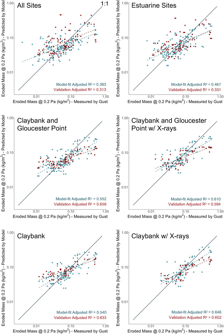
FIGURE A1. Blue circles and blue dashed line show performance for models with ΔAICc = 0 from each data subset in the Eroded Mass Model Set relative to a black 1:1 line. Red squares and red dashed line show validation model performance when half of the data were chosen to reset the models’ coefficients, and the same reset coefficients predicted erodibility using the other half of the data.
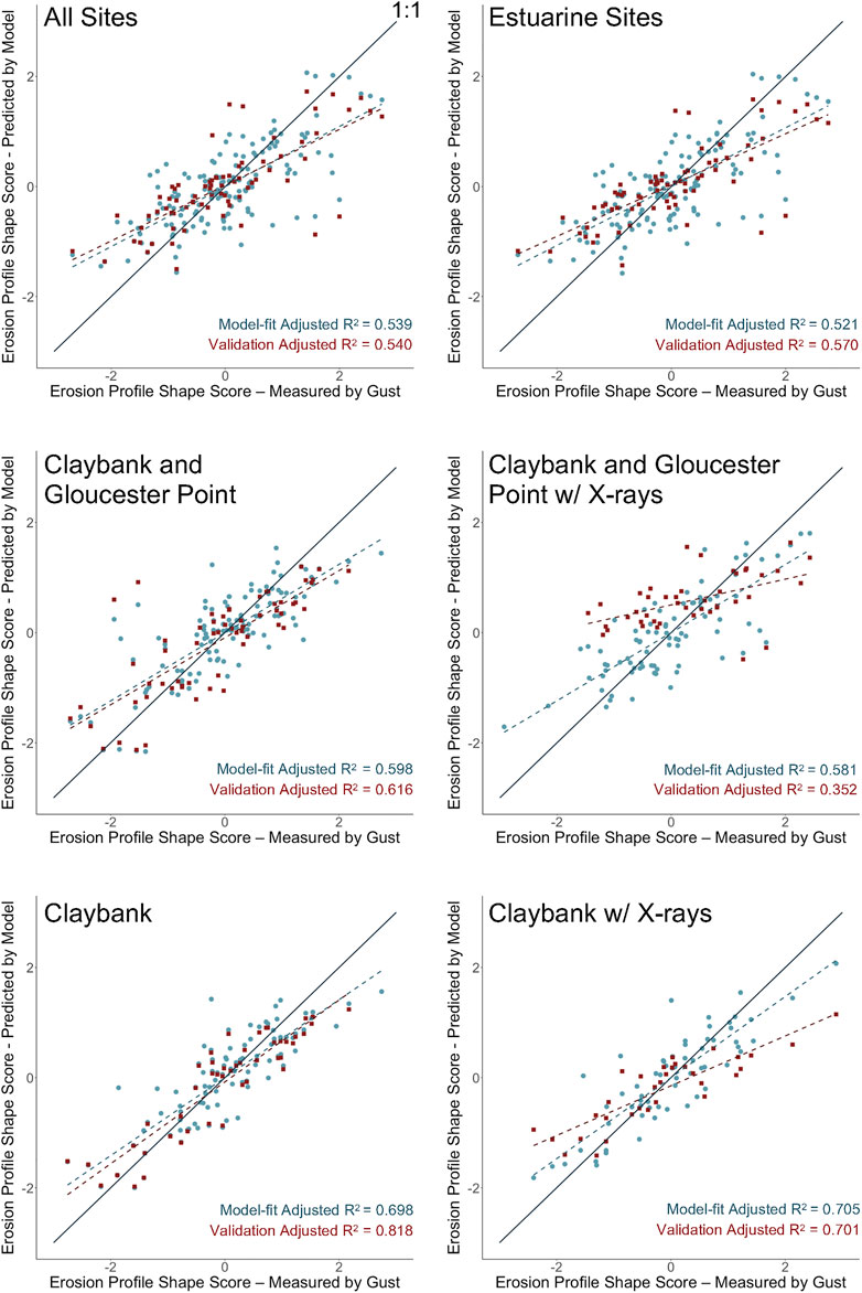
FIGURE A2. As in Figure A1, but for the Erosion Shape Model Set.
Keywords: bed erodibility, muddy sediment, bed properties, bed disturbance, estuarine hydrodynamics, multiple linear regression
Citation: Wright CL, Friedrichs CT and Massey GM (2022) Controls on Sediment Bed Erodibility in a Muddy, Partially-Mixed Tidal Estuary. Front. Earth Sci. 10:805130. doi: 10.3389/feart.2022.805130
Received: 29 October 2021; Accepted: 04 February 2022;
Published: 14 March 2022.
Edited by:
Andrew James Manning, HR Wallingford, United KingdomReviewed by:
Henry Bokuniewicz, The State University of New York (SUNY), United StatesCopyright © 2022 Wright, Friedrichs and Massey. This is an open-access article distributed under the terms of the Creative Commons Attribution License (CC BY). The use, distribution or reproduction in other forums is permitted, provided the original author(s) and the copyright owner(s) are credited and that the original publication in this journal is cited, in accordance with accepted academic practice. No use, distribution or reproduction is permitted which does not comply with these terms.
*Correspondence: Carl T. Friedrichs, Q2FybC5GcmllZHJpY2hzQHZpbXMuZWR1
Disclaimer: All claims expressed in this article are solely those of the authors and do not necessarily represent those of their affiliated organizations, or those of the publisher, the editors and the reviewers. Any product that may be evaluated in this article or claim that may be made by its manufacturer is not guaranteed or endorsed by the publisher.
Research integrity at Frontiers
Learn more about the work of our research integrity team to safeguard the quality of each article we publish.