Comparison of Phenology Estimated From Monthly Vegetation Indices and Solar-Induced Chlorophyll Fluorescence in China

Phenology is an important biological indicator for monitoring terrestrial ecosystems and global change. Solar-induced chlorophyll fluorescence (SIF) emitted by chlorophyll has been proven to characterize vegetation photosynthesis and phenology. In this study, we used monthly normalized difference vegetation index (NDVI), enhanced vegetation index (EVI), and SIF products to qualitatively compare the effectiveness at detecting the phenological characteristics (SOS (start-of-season), EOS (end-of-season), and LOS (length-of-season)) over China during 2007–2013. The phenological characteristics determined by gross primary productivity (GPP) were applied as the reference to validate the phenological characteristics derived from NDVI, EVI, and SIF. The results demonstrated that the phenological characteristics derived from SIF were more consistent with that of GPP than VIs (NDVI and EVI) when considering all latitude grades, different elevation grades, and different land cover types in China. In the middle- and high-latitude regions, SOS derived from the vegetation indices (SOS_VIs) did not deviate from those from GPP (SOS_GPP) and SIF (SOS_SIF), while in low latitudes, SOS_VIs were about 20 d later than SOS_SIF and SOS_GPP. The VIs (EOS_VIs) had a severe lag behind those of SIF (EOS_SIF) in estimating the EOS at all latitudes. The EOS_SIF had a deviation of fewer than 5 d compared with EOS estimated by GPP (EOS_GPP), whereas the deviation of EOS_VIs from EOS_GPP was about 10–31 d across low to high latitude regions. The biases of SIF and VIs were due to the inconsistency between vegetation photosynthesis and leaf greenness. Also, VIs overestimated the LOS at all latitudes, the difference of LOS between estimated by NDVI and estimated by GPP was as long as 39 d in the high-latitude region. Our study suggests that SIF is suitable for estimating the phenological characteristics of vegetation regardless of different latitudes, elevation grades, and land cover types in China, providing a basis for SIF to study the vegetation phenological characteristics in a regional scope.

Introduction

Vegetation phenology is a significant factor in measuring the dynamic change of vegetation (Zhao et al., 2015) and influences such things as the terrestrial energy exchange and the global carbon cycle (Keenan et al., 2014; Tang et al., 2015). Research on vegetation phenology can further our understanding of the change of seasonal phenomena (Vrieling et al., 2013), agricultural production (Tao et al., 2006), and global change (Cleland et al., 2007). Vegetation phenology is especially strongly correlated with climatic fluctuation (Richardson et al., 2013). Global climate change seriously affects the growth of terrestrial vegetation and changes the distributions, growth cycles, and species composition of vegetation (Zhao et al., 2015). Therefore, accurate monitoring of phenology is of great significance for understanding the exchange of material and energy between vegetation and climate as well as for the accurate assessment of vegetation productivity and the global carbon budget (Piao et al., 2006; Yu et al., 2017).

Vegetation gross primary productivity (GPP) is the total photosynthetic CO₂ fixation of vegetation at the ecosystem level (Xia et al., 2015). Several studies reported that canopy phenology (using the camera) was consistent with the phenology from GPP observations in the field, such as Bartlett Experimental Forest and Howland Forest in the United States (Richardson et al., 2009), the Lägeren Forest in northern Switzerland, and the Hainich Forest in central Germany (Ahrends et al., 2009). Therefore, GPP has been widely used as a reference for land surface phenology derived from satellite data analysis (Gonsamo et al., 2012; Jeong et al., 2017; Noumonvi et al., 2021).

In the past three decades, phenological vegetation information was monitored through time-series vegetation index data, which were obtained from satellite sensors, because these data have advantages in high temporal resolution and wide spatial coverage (Yu et al., 2017). Examples include the National Oceanic and Atmospheric Administration’s (NOAA’s) Advanced Very High-Resolution Radiometer (AVHRR) (Justice et al., 1985; Reed et al., 1994), Landsat (Melaas et al., 2013), MODerate Resolution Imaging Spectroradiometer (MODIS) (Zhang et al., 2003; Keenan et al., 2014; Walther et al., 2016), and Satellite Pour l’Observation de la Terre (SPOT) VEGETATION (Myneni et al., 1997; Zhou et al., 2001; Zhao et al., 2016). The normalized difference vegetation index (NDVI), which is associated with the greenness, seasonal, and interannual variabilities in most vegetation growth and activity, has been widely applied in the seasonal dynamic characteristics research on vegetation from the regional scale to the global scale (Tucker, 1979; Piao et al., 2006; Melaas et al., 2013). Compared with NDVI, the enhanced vegetation index (EVI) is less prone to saturation, which is caused by the luxuriant vegetation, and thus there are also many studies using EVI to observe vegetation growth (Sims et al., 2006; Testa et al., 2018). Although satellite vegetation indices (VIs)-based phenology is widely used to monitor seasonal growth and productivity of vegetation except for evergreen forests (Keenan et al., 2014; Testa et al., 2018), inconsistencies have been found between reflectance-based phenology and true vegetation photosynthesis based on ground observation (Churkina et al., 2005; Joiner et al., 2014; Cui T. et al., 2017; Jeong et al., 2017; Sun et al., 2018). In addition, NDVI-based phenological characteristics have also led to a longer length-of-season (LOS) than that derived by gross primary productivity due to an earlier estimated start-of-season (SOS) and later estimated end-of-season (EOS) in Harvard Forest (Gonsamo et al., 2012; Jeong et al., 2017; Lu et al., 2018). These discrepancies could be explained by the differences in temporal and spatial scales and dissimilarity between vegetation greenness and functions (Kross et al., 2011; Zhang et al., 2017). It has been suggested that the reflectance-based phenological detection method may not be an accurate proxy for plant photosynthesis (Frankenberg et al., 2011; Yang et al., 2014), and therefore, additional observations to help detect photosynthetic activity are necessary.

More recently, satellite remote sensing of solar-induced chlorophyll fluorescence (SIF) observations provides a new method for monitoring plant photosynthetic activities (Frankenberg et al., 2011; Guanter et al., 2014). SIF is a by-product of the photosynthesis process of a plant, and approximately 1% of absorbed photosynthetically active radiation (APAR) is re-emitted at a longer wavelength (640–850 nm) by chlorophyll, which has two emission peaks: a red spectral region with a peak at approximately 685 nm and a near-infrared region (NIR) with a maximum at approximately 740 nm (Wagle et al., 2016; Lu et al., 2018). Using high spectral resolution spectrometers and the advanced retrieval methodology based on the exploitation of Fraunhofer lines, SIF can be retrieved from platforms such as the Greenhouse gases Observing SATellite (GOSAT) (Frankenberg et al., 2011; Guanter et al., 2012), Global Ozone Monitoring Instrument-2 (GOME-2) (Joiner et al., 2013; Zhang et al., 2016), Orbiting Carbon Observatory (OCO-2) (Frankenberg et al., 2014; Li and Xiao, 2019), and TROPOspheric Monitoring Instrument (TROPOMI) (Guanter et al., 2015). Considering the longer time series of GOME-2 data, a number of studies applied it for long time-series research (Zhang et al., 2014; Cui Y. et al., 2017; Hu and Mo, 2020).

SIF data showed a significant positive linear relationship with GPP across the growing season, which suggests that SIF has good predictability for GPP from the canopy to satellite measurements (Damm et al., 2015; Yang et al., 2017; Li et al., 2018). Furthermore, some studies have shown that SIF could estimate the onset of spring and decline of photosynthesis in autumn more accurately in different biomes and regions, and thus can effectively estimate vegetation phenology (Joiner et al., 2014; Huang et al., 2021). Moreover, SIF had been demonstrated to be more sensitive for tracking short-term changes in GPP than reflectance-based vegetation indices (Damm et al., 2010; Yang et al., 2015; Luus et al., 2017; Sinha et al., 2017). However, most of the previous research using SIF to assess the vegetation phenology focused on the regions in relatively high latitude, in which the phenology is easily detected by SIF, few studies have compared vegetation indices and SIF in estimating phenological characteristics over a lengthy period at various latitudes. Also, few works estimated the phenology in different types of land cover or elevations in China (Jiao et al., 2020; Cheng et al., 2021).

In this study, we looked to quantify the improvement in detecting phenology by using SIF compared to NDVI and EVI products in different land cover types (evergreen forests, deciduous forests, shrublands, grasslands, and croplands), elevation grades (divided into 10 levels, according to the equal number of pixels [Supplementary Table S1]), as well as latitudes (high- (>40°N), middle- (30°N–40°N), and low- (<30°N) latitude regions). The reason for latitude grades division is in Synchronization of seasonal fluctuations between GPP and SIF, as well as VIs in each grid cell over China in China (Figure 1). Specifically, we compared phenological characteristics derived from MODIS NDVI data with those derived from GOME-2 SIF data in deciduous forests, shrublands, grasslands, croplands, and evergreen forests using GPP data obtained from MODIS and the Max Planck Institute (MPI) as references. Considering that SIF data has been available since 2007, and GPP data accessed by MPI is only available until 2013, thus we limit the study year to 2007–2013. The main objectives of this research are twofold. One is to compare the performance of SIF-based and NDVI-based satellite remote sensing data in monitoring the satellite-GPP-based vegetation photosynthesis. The other is to study the phenological characteristics of SIF and NDVI in different regions (different latitudes, elevations, and land cover types), taking GPP as the reference.

FIGURE 1

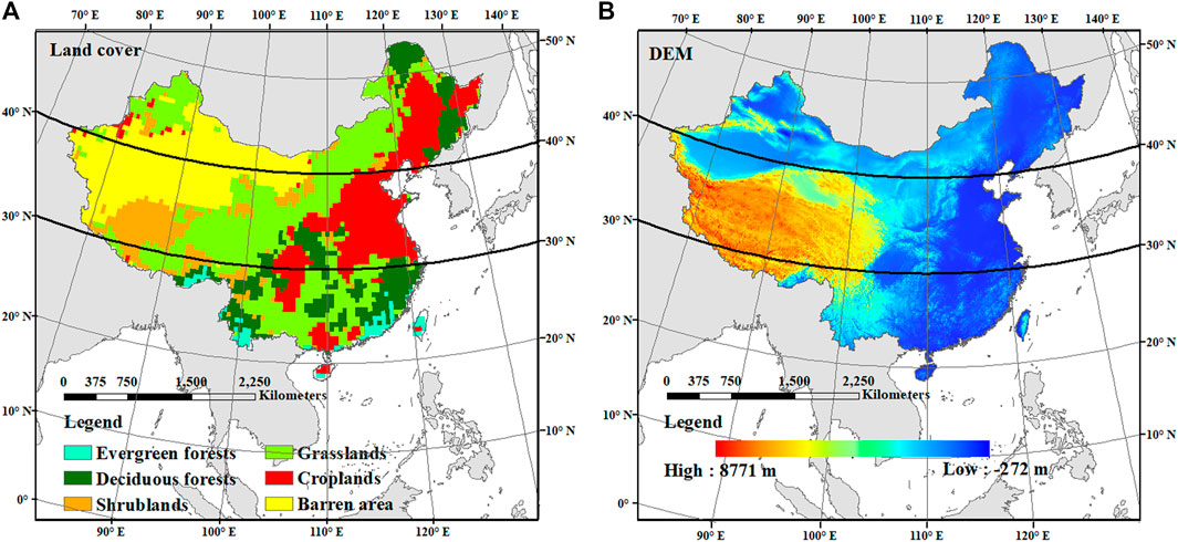
FIGURE 1. Land cover map (A) and DEM (B) of China. The land cover was reclassified into evergreen forests, deciduous forests, shrublands, grasslands, croplands, and barren areas. The spatial resolution of the land cover map is processed to 0.5° × 0.5°. The study area was divided into the high-, middle-, and low-latitude regions by the bold and solid lines in the two panels.

Materials and Methods

Vegetation Indices Data

The monthly NDVI and EVI data from 2007 to 2013 were provided by the MODIS Terra Vegetation Indices dataset (MOD13C2) with a spatial resolution of 0.05°×0.05°. The MODIS NDVI dataset is based on specific spectral bands (red and infrared) designed to offer stable global vegetation leaves greenness monitoring. It has been widely used in land cover classification, carbon exchange modeling, and phenology studies (Shen et al., 2014; Aredehey et al., 2017; Biudes et al., 2021). In addition, EVI is more sensitive to high biomass areas and is minimally impacted by soil and atmosphere due to the increased blue band information (Huete et al., 2002; Jiang et al., 2008). Therefore, both NDVI and EVI were selected for phenological research in this study. In addition, NDVI and EVI were spatially resized to 0.5°×0.5° grid cells using the bilinear resampling method to make it consistent with the spatial resolution of SIF data.

Solar-Induced Chlorophyll Fluorescence Data

The SIF is acquired from the GOME-2 onboard the Eumetsat’s MetOp-A platform, a sun-synchronous orbit satellite whose nominal nadir footprint size is 40 × 80 km and spectral resolution is 0.5 nm with an equator crossing time of 9:30 a.m. (Joiner et al., 2014). The SIF signal is obtained primarily by the filling-in of solar Fraunhofer lines at wavelengths near 740 nm, which is the far-red fluorescence emission peak. A principal component analysis approach with a simplified radiative transfer model was used to separate the spectral signatures of atmospheric absorption and surface reflection from the SIF emission. The monthly SIF product had been cloud filtered and aggregated to 0.5°×0.5° spatial resolution by Joiner et al. (2013) and can be downloaded at http://avdc.gsfc.nasa.gov. In this study, we used version 2.7 Level 3 data from 2007 to 2013.

Gross Primary Productivity Data

The GPP data were used as the phenological reference from two different sources. One source of GPP product was data-driven derived from the MPI (GPP_MPI). Specifically, it was estimated by a statistical model to obtain GPP estimates by upscaling global FLUXNET eddy covariance observations with the climate forcing data set CRUNCEPv6 using a machine learning method (Tramontana et al., 2016; Jung et al., 2017). GPP_MPI has been widely used for GPP validation in many pieces of research (Frankenberg et al., 2011; Jung et al., 2011; Guanter et al., 2014; Jiang and Ryu, 2016). A more detailed description of GPP_MPI is given in Tramontana et al. (2016). The monthly global GPP data set at the 0.5° resolution, covering 2007–2013, was downloaded from www.bgc-jena.mpg.de/geodb/projects/Data.php.

The second source of GPP data was the MODIS GPP product (GPP_MOD), which is calculated by using the MOD15A2 fraction of photosynthetically active radiation (fPAR) product and meteorological data, and applying the semi-empirical method (Running et al., 2004). In this study, we downloaded the MOD17A2 monthly product with a spatial resolution of 0.05°, which was accessed from the Numerical Terra dynamic Simulation Group (NTSG), covering the years 2007–2013. The data was downloaded from http://files.ntsg.umt.edu/data/NTSG_Products/MOD17/GeoTIFF. Then, the bilinear resampling method was used to resize the spatial resolution of GPP to 0.5°×0.5° grid cell, which was consistent with the spatial resolution of SIF data.

Ancillary Data

The land cover data set was obtained from the MODIS dataset (MOD12Q1), the University of Maryland (UMD) land cover classification type was chosen and downloaded from http://files.ntsg.umt.edu/data/NTSG_Products/MOD17/GeoTIFF/MOD12Q1/.

Temperature data were from Earth System Research Laboratory (ESRL) Physical Sciences Division (PSD) (www.esrl.noaa.gov/psd/data/gridded/data.UDel_AirT_Precip.html). We chose the global long-term monthly means V4.01 data which covers 2007–2013, with the spatial resolution of 0.5°×0.5°.

Digital elevation data were generated from the CGIAR Consortium for Spatial Information (CGIAR-CSI) Shuttle Radar Topography Mission (SRTM) version 4.1 with a spatial resolution of 250 × 250 m. The elevation files have been mosaiced into a seamless near-global coverage (up to 60° north and south) and downloaded from https://cgiarcsi.community/.

Land cover data were spatially resampled to 0.5°×0.5° grid cells by the majority algorithm to be consistent with the spatial resolution of SIF and GPP_MPI data, while elevation data were resampled by the mean resampling method.

Phenological Characteristics Extraction

To estimate vegetation phenological characteristics, the monthly SIF, VIs, GPP_MPI, and GPP_MOD data are smoothed and interpolated into a daily scale by the spline method (Chen et al., 2004), then normalized the daily scale data. In order to reduce noise and extract vegetation phenological characteristics from time-series data accurately, the Savitzky-Golay smoothing model (Chen et al., 2004; White et al., 2009; Brown et al., 2010; Zhao et al., 2016) was applied to the original SIF, VIs (NDVI and EVI), GPP_MPI, and GPP_MOD time series data. Smoothed and daily interpolated data have been applied to estimate fluctuation of vegetation growth or vegetation phenological characteristics with high accuracy (Jonsson and Eklundh, 2002; Piao et al., 2006; Zhang et al., 2013; Jeong et al., 2017; Chang et al., 2019; Wang et al., 2019). They have demonstrated that monthly data could provide a reliable result in phenological characterizing. The data used in this study were normalized by the annual maximum and minimum data to fill the magnitude gap among different data.

Then, the SOS, EOS, and LOS were estimated based on the daily SIF, VIs, GPP_MPI, and GPP_MOD. In this study, we defined SOS or EOS as a rapid continuous increase or decrease in remotely sensed time-series data after the long annual period of photosynthetic senescence (White et al., 2009). Thus, we adopted the threshold determined by White et al. (1997) which is the 50% point of annual normalized time series seasonal curve to calculate the phenology characteristics, because this threshold has been verified as being sensitive to the dynamics of underlying vegetation, canopy cover, and structure (Richardson et al., 2009; de Beurs and Henebry, 2010; Lu et al., 2018). We also calculated the LOS, which is the difference between the SOS and EOS. The schematic diagram of the phenological estimation method is shown in Figure 2, the intersection points of the 50% threshold line (the red horizontal dotted line) and the preprocessing seasonal curve (the black solid line) corresponded to SOS and EOS. Especially, the croplands in the middle-latitude region are planted twice a year, thus we estimate the first and last time to reach the 50% threshold as the SOS and EOS of these regions.

FIGURE 2

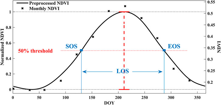
FIGURE 2. The method of estimating phenological characteristics. The “×” points are original data. The black solid line is a preprocessed seasonal curve that has been smoothed, interpolated, and normalized. The red horizontal dotted line is the 50% threshold of maximum and minimum of the preprocessed seasonal curve (the red vertical dotted line). The blue square dots are the SOS and EOS, and LOS is the difference between SOS and EOS.

Due to the data series being at the monthly temporal resolution, it may cause some deviation from the daily data in estimation phenology characteristics in the daily unit. The flux site GPP data, which has both monthly and daily data, were used to estimate the phenology characteristics, using Savitzky-Golay smoothing and spline interpolation, to determine the uncertainty of the data with different temporal resolutions, as Supplementary Figure S1 shows. It is found that after the preprocessing, the SOS and EOS derived from the daily data were 8 d different from the monthly data.

Resampling all the remotely sensed data to 0.5° spatial resolution may lead to some mixed pixels in the images, but the effect of the resampling was limited as Supplementary Figure S2 shows. The EOS from the GPP_MOD data was calculated with 0.05° (Supplementary Figure S2A) and 0.5° (Supplementary Figure S2B) spatial resolutions. We can find that the EOS distributions were not changed significantly before and after resampling. Supplementary Figure S2(C) shows the histograms of the calculated EOS. The histograms from different resolutions data were also similar, which indicates that the uncertainty from resampling preprocessing did not affect the phenology characteristics significantly.

Quantifying Synchronicity Methods

To quantify the synchronization of seasonal fluctuations of GPPs (GPP_MPI and GPP_MOD), SIF, and VIs (NDVI and EVI), the mean absolute error (MAE, as Eq. 1) was conducted. In detail, we calculated MAE on monthly normalized SIF, NDVI, and EVI with GPP_MPI and GPP_MOD during spring and autumn (March, April, May, September, October, and November) in each grid cell from 2007 to 2013.

$MAE= \frac{1}{n} {\displaystyle \sum }_{i=1}^n\left|y_i- x_i\right| (1)$

where $y_i$ represents the i-th GPP value in a grid cell, x_i represents the i-th SIF, NDVI, and or EVI value in the grid cell at the same position, and n is the number of GPP-SIF(/NDVI/EVI) value pairs.

Results

Synchronization of seasonal fluctuations between GPP and SIF, as well as VIs in each grid cell over China

To explore the synchronization of the seasonal curves of GPPs and SIF, as well as GPPs and VIs in the period of vegetation leaf development and leaf senescence, the spatial distributions of MAE in spring and autumn are shown in Figure 3. The MAE values between GPPs and SIF (Figure 3A for GPP_MPI and Figure 3D for GPP_MOD), NDVI (Figure 3B for GPP_MPI and Figure 3E for GPP_MOD), as well as EVI (Figure 3C for GPP_MPI and Figure 3F for GPP_MOD) are shown. This figure shows lower MAE values obtained from SIF and GPPs than that from VIs and GPPs, which suggests that SIF curves can produce more similar phenological characteristics to GPP. Therefore, SIF could provide a basis for the application of SIF to indicate vegetation phenological characteristics.

FIGURE 3

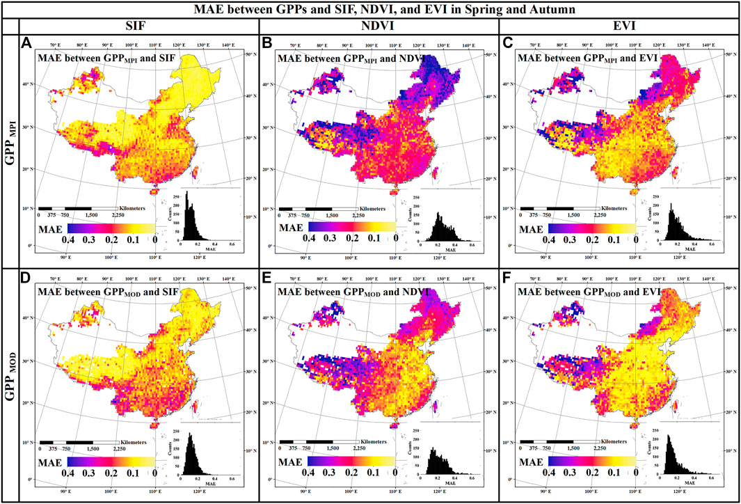
FIGURE 3. Spatial distributions of MAE between GPPs and SIF [(A) for GPP_MPI and (D) for GPP_MOD], GPPs and NDVI [(B) for GPP_MPI and (E) for GPP_MOD], as well as GPPs and EVI [(C) for GPP_MPI and (F) for GPP_MOD] in China during 2007–2013.

In addition, it was found that the synchronization between SIF and GPPs was differentiated in latitudes. SIF and GPPs showed high-level synchronicity in the high-latitude regions (>40°N), medium-level synchronicity in the middle-latitude regions (30°N–40°N), and relatively low-level synchronicity in the low-latitude regions (<30°N). The variation of the synchronizations provides a necessity to analyze the phenological characteristics by SIF at different latitudes. Therefore, the study area was divided into high-, middle-, and low-latitude regions, respectively. Meanwhile, the synchronicity between SIF and GPPs had some minor differences at the same latitude region, which might be caused by the influence of elevation and land cover types.

Seasonal Cycles of SIF and VIs at Different Latitudes

We analyzed the phenological seasonal cycles of different land cover types (deciduous forests, shrublands, grasslands, croplands, and evergreen forests) in different latitude regions (high-, middle-, and low-latitude regions) (Figures 4–6, and 9). The value of each point in these figures was the average monthly value of the corresponding land cover in the latitude region during the 2007–2013 period. We found that the seasonal dynamic curve of SIF was closer to that of GPPs, but the curve of VIs in autumn had a significant mismatch with the seasonal curves of two products of GPP in most cases. Figure 4 shows that the VIs curve ascended earlier than the other curves derived from GPPs in spring, while in autumn, it descended later than GPPs in the high-latitude region. Compared to GPPs, the SIF curve rose a little later than GPPs and fell together with GPPs. Although compared with NDVI and EVI, SIF had little advantage (±10 d) for estimating SOS, for autumn phenology, the difference between EOS_SIF (EOS estimated by SIF) and EOS_GPPs (EOS estimated by GPP_MPI and GPP_MOD) (about 3 d) was much smaller than that between EOS_VIs (EOS estimated by NDVI and EVI) and EOS_GPPs (about 31 d for NDVI and about 19 d for EVI). Almost all the phenological curves except croplands in the middle-latitude region rose together in spring (±10 d), while in autumn, the VIs curves fell behind SIF and GPPs (about 5 d for SIF, about 11 d for EVI, and about 22 d for NDVI), as shown in Figure 5. While in contrast to the SIF, GPP_MOD, and GPP_MPI, the seasonal cycle of VIs was delayed in both spring and autumn in the low-latitude region (Figure 6) on deciduous forests, shrublands, grasslands, and croplands. The difference between SOS_SIF (SOS estimated by SIF) and SOS_GPPs (SOS estimated by GPP_MPI and GPP_MOD) (about 5 d) was smaller than that between SOS_VIs (SOS estimated by NDVI and EVI) and SOS_GPPs (about 18 d for EVI and about 24 d for NDVI). Additionally, the difference between EOS_SIF and EOS_GPPs (about 4 d) was also smaller than that between EOS_VIs and EOS_GPPs (about 10 d for EVI and about 28 d for NDVI). This phenomenon can also be seen in Figure 9. Furthermore, the mismatch between SOS and EOS derived from VIs, GPPs, and SIF, especially the advance of SOS_VIs in the high-latitude region, and the serious delay of EOS_VIs in all latitudes would lead to an overestimation of LOS_VIs (LOS estimated by NDVI and EVI), especially the clear difference between LOS_NDVI (LOS estimated by NDVI) and LOS_GPPs (LOS estimated by GPP_MPI and GPP_MOD) was about 39 d in high latitudes. In a word, considering all cases, the bias of SIF estimation of phenological characteristics was minimal.

FIGURE 4

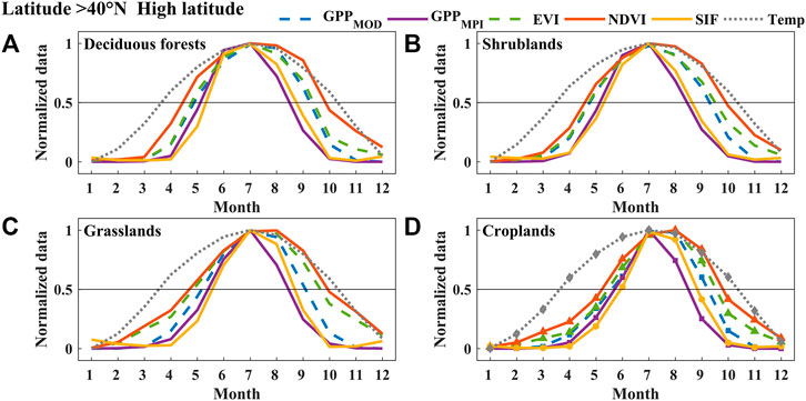
FIGURE 4. The normalized mean seasonal cycle of area-averaged GPP_MOD, GPP_MPI, NDVI, EVI, SIF, and Temperature (Temp) of deciduous forests (A), shrublands (B), grasslands (C), and croplands (D) in the high-latitude region (over 40°N) of China between 2007 and 2013. Error bars in all subplots represent the monthly standard deviations during 2007–2013.

FIGURE 5

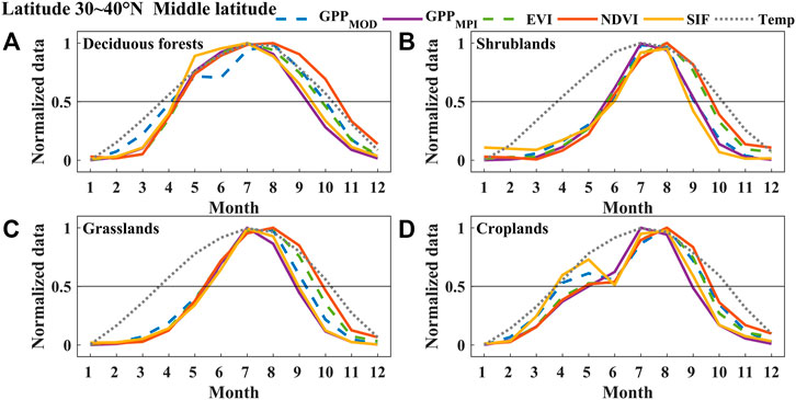
FIGURE 5. The normalized mean seasonal cycle of area-averaged GPP_MOD, GPP_MPI, NDVI, EVI, SIF, and Temperature (Temp) of deciduous forests (A), shrublands (B), grasslands (C), and croplands (D) in the middle-latitude region (31–40°N) of China between 2007 and 2013. Error bars in all subplots represent the monthly standard deviations during 2007–2013.

FIGURE 6

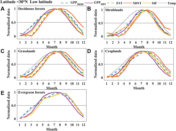
FIGURE 6. The normalized mean seasonal cycle of area-averaged GPP_MOD, GPP_MPI, NDVI, EVI, SIF, and Temperature (Temp) of deciduous forests (A), shrublands (B), grasslands (C), croplands (D), and evergreen forests (E) in the low-latitude region (below 31°N) of China between 2007 and 2013. Error bars in all subplots represent the monthly standard deviations during 2007–2013.

The annual changes of GPP_MPI, GPP_MOD, SIF, and NDVI as well as EVI of evergreen forests over 7 years (2007–2013) are shown in Supplementary Figure S3. It was found that the changes in NDVI and EVI throughout the year are very apparent. The difference between the maximum and minimum values of NDVI did not exceed 0.15, as well as that of EVI, was no more than 0.2, and the upward and downward trends were not very distinct. Thus, it is difficult to distinguish SOS and EOS through VIs in the evergreen region. However, SIF showed a clear upward trend from March to May and a significant downward trend from September to November, which was the same as the changing trend of the two sources of GPP, and the phenological change trend could be distinguished. Therefore, the phenological characteristics estimated by SIF (Figure 6E, Figure 7, Figure 8, Figure 9, and Figure 10; Supplementary Figures S4 and S5) of the evergreen forests are displayed, but would not be compared with VIs in the results.

FIGURE 7

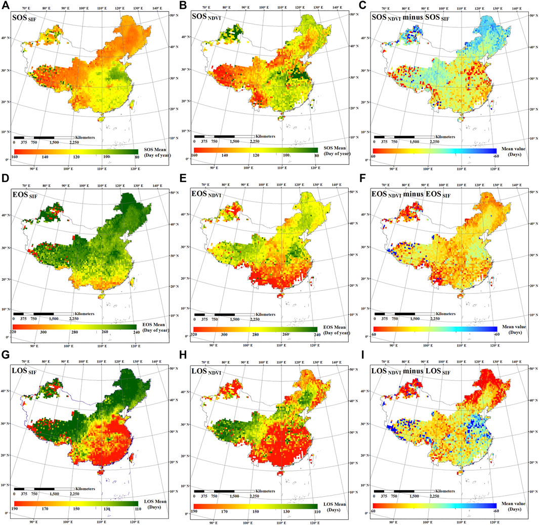
FIGURE 7. Spatial distributions of 7-years averaged SIF and NDVI-based SOS (A, B), EOS (D, E), and LOS (G, H) dates, the difference between NDVI and SIF-based SOS (C), EOS (F), and LOS (I) dates in China during 2007–2013.

FIGURE 8

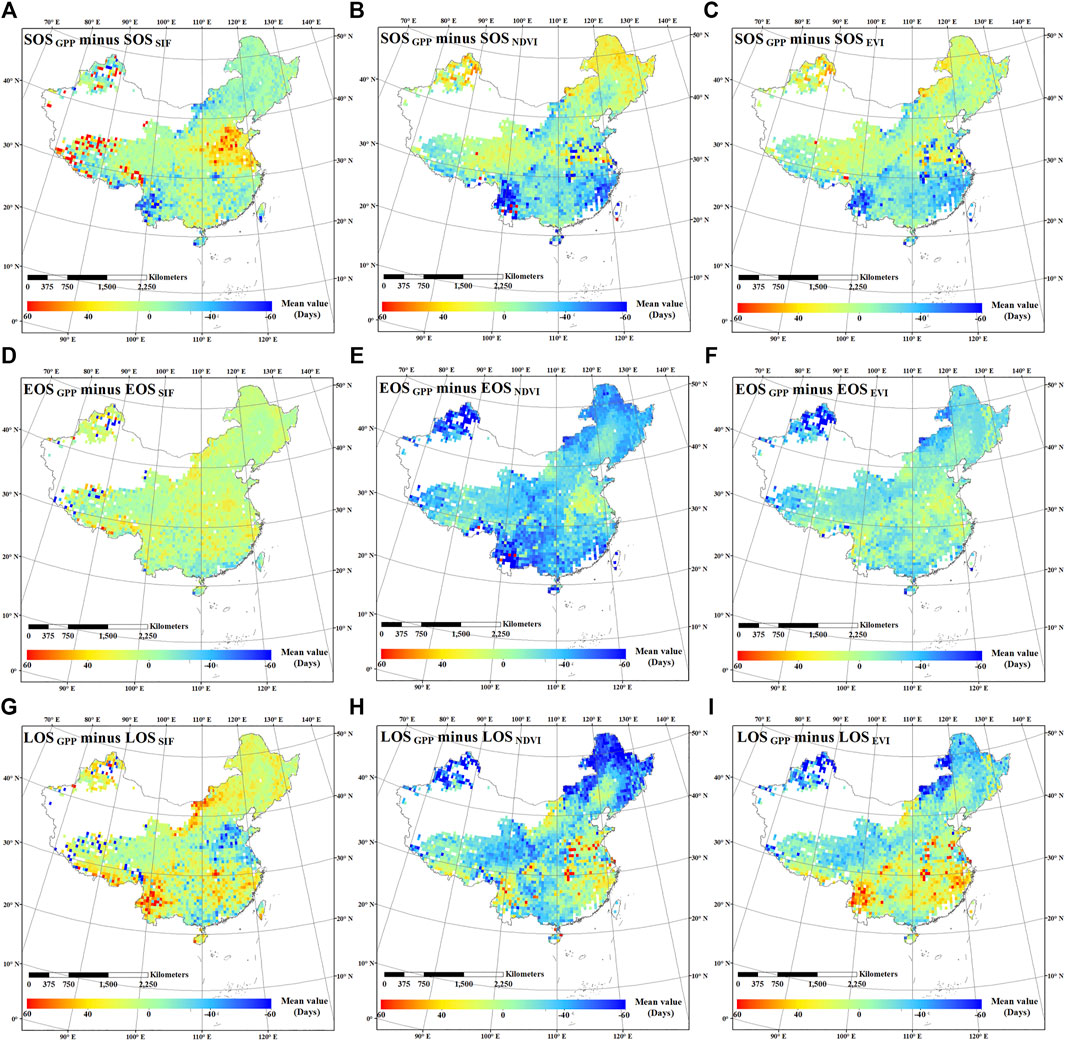
FIGURE 8. Spatial distributions of the difference between SOS_GPP and SOS_SIF (A), EOS_GPP and EOS_SIF (D), and LOS_GPP and LOS_SIF (G), the difference between SOS_GPP and SOS_NDVI (B), EOS_GPP and EOS_NDVI (E), and LOS_GPP and LOS_NDVI (H), and the difference between SOS_GPP and SOS_EVI (C), EOS_GPP and EOS_EVI (F), and LOS_GPP and LOS_EVI (I) in China.

FIGURE 9

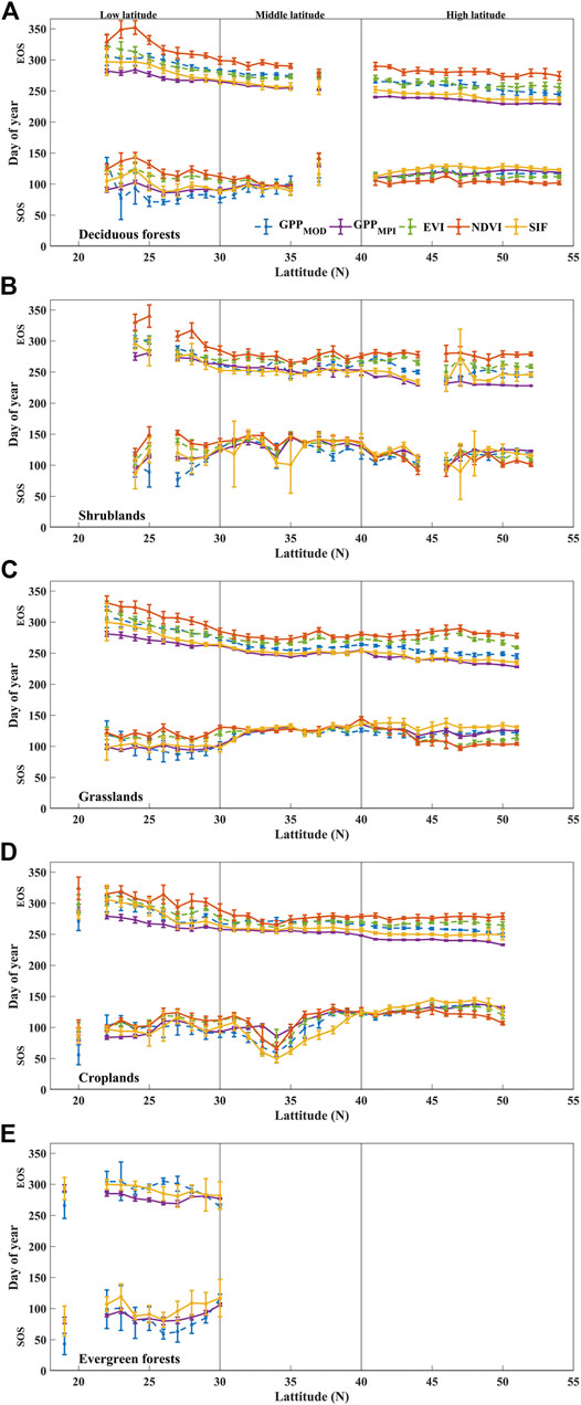
FIGURE 9. The area-averaged SOS (the lower lines) and EOS (the upper lines) of GPP_MOD, GPP_MPI, NDVI, EVI, and SIF over deciduous forests (A), shrublands (B), grasslands (C), croplands (D), and evergreen forests (E) during 2007–2013 in China. The points and error bars in all subplots represent the mean and standard deviations for 2007–2013, respectively.

FIGURE 10

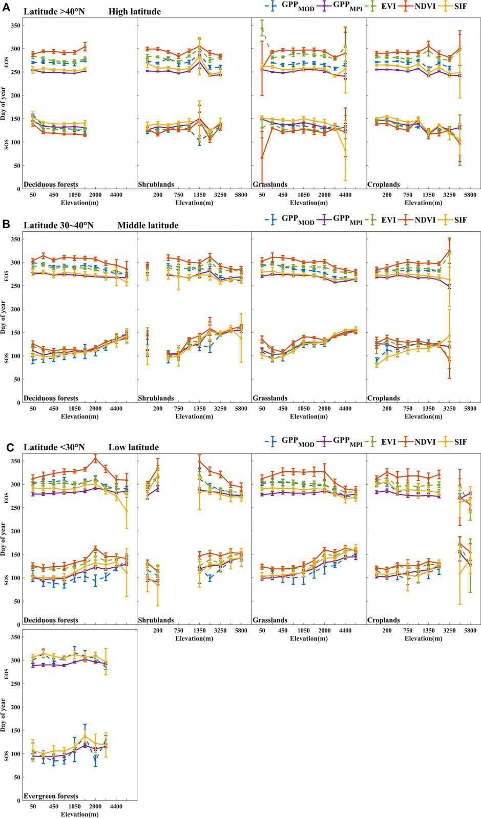
FIGURE 10. The area-averaged SOS (the lower lines) and EOS (the upper lines) of GPP_MOD, GPP_MPI, NDVI, EVI, and SIF over deciduous forests, shrublands, grasslands, croplands, and evergreen forests during 2007–2013 in high- (A), middle- (B), and low- (C) latitude regions. The points and error bars in all figures represent the mean and standard deviations for 2007–2013, respectively.

Spatial Distribution of Phenological Characteristics Estimated From SIF, VIs, and GPP

To analyze the spatial distribution of the phenological characteristics in China, the average values of SOS, EOS, and LOS based on SIF and NDVI and the difference between their estimations in deciduous forests, shrublands, grasslands, and croplands in China over 7 years (2007–2013) were mapped (Figure 7). In the high latitude areas, SOS_SIF was later than SOS_NDVI (SOS estimated by NDVI); in the low latitude areas, SOS_SIF was earlier than SOS_NDVI; while in the middle latitude areas, SOS_SIF was later than SOS_NDVI in the west and earlier in the east, which may be due to elevation effect. Except for a few anomalies, the EOS_SIF data was ahead of that of the EOS_NDVI (EOS estimated by NDVI) data for all of China. The advance of SOS and the delay of EOS has led to an overestimation of LOS_NDVI in most areas of China, except for croplands in the middle latitudes and a small area of Tibetan shrublands and grasslands. The spatial distribution of phenological characteristics estimated from EVI and the difference between SIF and EVI estimations were shown in Supplementary Figure S4. Compared with NDVI, the phenological characteristics estimated by EVI were closer to the phenological characteristics estimated by SIF. Overall, these results indicated that SIF and VIs are vastly different in estimating phenological characteristics.

The spatial distribution of the difference between the phenological characteristics estimated by GPP and those estimated by SIF, NDVI, and EVI are shown in Figure 8. The phenological characteristics of GPP were the average value of the two sources of GPP (GPP_MOD and GPP_MPI) estimated phenological characteristics. It was found that the phenological characteristics estimated by SIF were more similar to those estimated by GPP, and the difference was within ±40 d. However, the difference between the phenological characteristics estimated by NDVI and those estimated by GPP was the largest. Most of the differences were delayed (that is, the difference was negative), with a difference of more than 40 d in many regions. The difference of the phenological characteristics estimated by EVI and GPP is a little smaller than that between NDVI and GPP. However, the estimated date was still delayed in many areas. Compared with VIs, SIF had the advantage to estimate EOS in that the difference between EOS_SIF and EOS_GPP was the smallest. EOS_VIs had delayed estimation in almost the entire study area, distinguishing between −40 and −60 d in many areas. This also leads to an overestimation of LOS_VIs, especially in high latitudes, and where the difference is around −50 d. Supplementary Figure S5 shows the frequency statistics of Figure 8, and it could also be found that SIF is more suitable than VIs in estimating vegetation phenological characteristics.

Phenological Characteristics Estimated From SIF and VIs With GPP as a Reference in Different Land Covers

Figure 9 represents the phenological characteristics derived from different datasets (SIF, NDVI, EVI, and GPP) in different land covers along latitudes. Different land cover types showed distinct SOS and EOS changes along with latitudes. For example, the SOS shifted to an earlier date and EOS delayed gradually for deciduous forests and grasslands from high to low latitudes and resulted in a longer LOS in lower latitudes. Nevertheless, for shrublands and croplands, the curves undulated intensively with the latitude change. For instance, the estimated SOS for croplands, especially in the middle-latitude region, showed a “concave”. The reason may be intensive planting twice a year in central China, the phenology trend represents a two-peak pattern (Figure 5D). In addition, since evergreen forest only appears in low latitudes, this study did not show the variation in middle and high latitudes.

However, the land cover types did not influence the difference in the estimation of phenological characteristics between SIF and VIs compared with GPP. Specifically, the difference between SIF and GPP is smaller than the difference between VIs and GPP in different land cover types. The differences of 7-years averaged SOS, EOS, and LOS between the NDVI and GPP, EVI, and GPP, as well as SIF and GPP are shown in Supplementary Figure S5. The phenological characteristics of GPP were the average value of the GPP_MOD and GPP_MPI estimated phenological characteristics. The frequency of difference values above the total and different land cover types by pixel were counted in this figure. The distribution curve conformed to an approximately normal distribution, and frequency distributions of different land cover types were similar to total frequency distribution. The differences between SIF and GPP phenological characteristics were more concentrated and closer to 0, while there was systematic bias between VIs and GPP phenological characteristics, and this caused the differences to be far from 0, especially in EOS. It manifested that SIF-estimated SOS, EOS, and LOS were all consistent with that estimated from GPP regardless of the land cover type. Conversely, the VIs-estimated SOS, EOS, and LOS were further away from those derived from GPP. The above results further proved that SIF is more available for estimating phenological characteristics in most land covers in China.

Phenological Characteristics Estimated From SIF and VIs With GPP as a Reference in Different Elevations

Figure 10 shows the variation of SOS and EOS with elevation in different land cover types and different latitude regions. Overall, the phenological characteristics have the same tendency with the elevation rising, the SOS of the vegetation becomes later, the EOS is earlier, and the vegetation growth period is shortened. This phenomenon is particularly pronounced in the middle- and low-latitude regions, possibly because the temperature at these latitudes is strongly influenced by the elevation. In the middle- and low-latitude regions, the average elevation of the Qinghai-Tibet Plateau in the west of the study area can reach about 6000 m, while the elevation in the eastern coastal area is only about 0 m. The great variation of elevation would result in significant temperature differences, and the vegetation phenology will also change. In the high-latitude region, the variation of elevation is not clear, which may be due to the relatively small difference in elevation, and the lower temperature in high latitudes. However, the differences between SOS_VIs and SOS_SIF (or SOS_GPPs) and between EOS_VIs and EOS_SIF (or EOS_GPPs) have always existed. That is, the SOS and EOS derived from VIs deviated more from SIF and GPPs in most elevations.

Discussion

The phenological changes of GPPs and SIF were consistent among the high-, middle-, and low-latitude regions, while the seasonal fluctuations of VIs were largely different from those of GPPs (Figures 4–6). In the high-latitude region, SOS_VIs and SOS_SIF were both close to SOS_GPPs, but SOS_VIs was always earlier than SOS_SIF, whereas in the middle-latitude region, the seasonal curves of VIs rose synchronously with SIF and GPPs in spring phenology. However, in the low-latitude region, the VIs-based spring phenology has a lag to the SOS estimated by SIF and GPP. Meanwhile, VIs largely lagged behind SIF or GPPs in the estimation of autumn phenological characteristics at high to low latitudes, especially EOS_NDVI. The estimated phenological characteristics by SIF in the high-latitude region were consistent with the results of previous research, in which NDVI showed an advance in spring and a distinct lag to GPP and SIF in autumn were found over northern forests (Jeong et al., 2017) or a specific forest such as Harvard Forest (Lu et al., 2018). Walther et al. (2016) also verified a similar seasonal change over deciduous broadleaf forests in the middle latitude along the east coast of North America, that is, NDVI lagged behind GPP, while SIF was synchronized with GPP. The distinct bias of VIs, compared with SIF, in estimating phenological characteristics might be due to the time inconsistency between photosynthesis and greenness. VIs generally indicated the greenness of vegetation, while SIF is closely related to vegetation photosynthesis. In spring, vegetation in the high- and middle-latitude regions might require time to photosynthesize and increase primary productivity by assimilating carbon after leaf emergence (Kikuzawa, 2003; Jeong et al., 2017). In addition, it caused a rapid increase in VIs values, but a slow increase in SIF and GPP values in the sprouting period. However, the result that SIF had an absolute advantage to estimate the spring phenological characteristics based on GPP in the low-latitude region is different from that in the high- and middle-latitude region and is still to be explained. On the other hand, EOS_VIs have a lag at high to low latitudes, which may be due to the fact that VIs estimate vegetation phenology by tracking vegetation characteristics such as leaf area index and chlorophyll content and could not reflect slight phenological changes in time in autumn (Lu et al., 2018). In the case of autumn, carbon assimilation and SIF are mainly limited by sunlight or suitable temperature availability (Suni et al., 2003; Medvigy et al., 2013; Jeong and Medvigy, 2014; Wang et al., 2020), while vegetation indices are different from SIF, which are primarily controlled by the air temperature (Wang et al., 2020; Yang et al., 2020). Thus, the leaves may drop after the photosynthesis has begun to decrease, which results in distinct lags in VIs, but a synchronized change with GPP in SIF (Daumard et al., 2010). Especially, EOS_NDVI significantly lags behind other sources of data (GPPs, SIF, and EVI), possibly because NDVI was reported to have saturation effects in high biomass canopies (Walther et al., 2016) and it starts decreasing after a large number of leaves become senescent and drop.

In addition, the phenological characteristics estimation of croplands in middle-latitude regions was only identified on the first and last date with the values of 50% thresholds as SOS and EOS. This may not be appropriate because the crops are always harvested two times per year. To detect the double peaks in mid-latitude croplands is our task in future studies.

SIF has also been proven reliable to track GPP phenological fluctuations in evergreen forests, as shown in Supplementary Figure S3. This finding supports the viewpoint of Magney et al. (2019) that a good correlation between SIF and GPP in Colorado subalpine evergreen coniferous forests enables SIF and GPP to track each other consistently. The large seasonal variations in SIF yield highlight its unique ability to accurately track the seasonality of photosynthesis in different land covers, even in evergreen forests, which was not detected successfully by VIs.

Furthermore, since the temperature is one of the important climatic factors affecting vegetation phenology (Cong et al., 2013; Liang and Zhang, 2016; Lang et al., 2019; Han et al., 2020), the seasonal curve of temperature in the high-, middle-, and low-latitude regions in different land cover types is shown in Figures 4–6. We can find that the fluctuations of temperature were similar in the same latitude region in different land cover types, but the fluctuations of vegetation curves (GPPs, SIF, and VIs) were different, which indicated that the phenological characteristics of different vegetation have different sensitivities to temperature. For example, in the middle-latitude region, the seasonal fluctuations of deciduous forests were similar to the temporal change of temperature, whereas in shrublands and grasslands, the curves of GPPs, SIF, and VIs began to rise after about 2 months of temperature rise in spring. Moreover, by comparing the seasonal fluctuation of temperature and the curves of GPPs and SIF in various latitude regions, we found that the lower the latitude region, the higher the sensitivity of GPPs and SIF to temperature. These results are consistent with some previous studies (Doi and Takahashi, 2008; Gao et al., 2020). Therefore, the phenological characteristics calculated from the remotely sensed temperature have limitations in terms of the different responses of vegetation types to temperature, especially in the middle to high latitudes.

Overall, our research showed the fact that SIF tracked the variation in vegetation phenology more accurately than VIs in different latitudes, elevations, and land cover areas based on monthly data in China.

Conclusion

In this study, we compared and analyzed the discrepancies of phenological characteristics derived from GOME-2 SIF product and MODIS VIs products in China from 2007 to 2013. SIF showed more effectiveness in estimating the phenological characteristics than VIs in different latitudes, elevations, and land cover areas in China. The phenological curves of VIs and SIF in the high- and middle-latitude regions rose together in spring, while the VIs curve lagged far behind SIF in autumn. In the low-latitude region, in contrast to the SIF and GPP, the seasonal cycles of VIs were delayed in both spring and autumn. Thus, SIF appears to be a better option to accurately estimate the characteristics of vegetation phenology and the phenological changes. This provides a basis for future research on the application scenarios of using SIF data to describe vegetation growth conditions and analyze vegetation phenological characteristics. Moreover, the obviously different phenological changes between VIs and SIF in the high-latitude region, middle-latitude region, and low-latitude region provided evidence for future research on the relationship between vegetation photosynthesis and vegetation greenness across latitudes.

Data Availability Statement

The original contributions presented in the study are included in the article/Supplementary Material, further inquiries can be directed to the corresponding authors.

Author Contributions

XW, SL, and ZS designed the study; XW performed the analysis; XW and SL interpreted the data results; XW and ZZ drafted the original manuscript; SL, ZZ, and SZ acquired funding; and all authors contributed to the results and reviewed and edited the manuscript.

Funding

This research was funded by the National Natural Science Foundation of China (41971290, 41977407, 41671347, and 41001258) and the Fundamental Research Funds for the Central Universities (130014925).

Conflict of Interest

The authors declare that the research was conducted in the absence of any commercial or financial relationships that could be construed as a potential conflict of interest.

Publisher’s Note

All claims expressed in this article are solely those of the authors and do not necessarily represent those of their affiliated organizations, or those of the publisher, the editors, and the reviewers. Any product that may be evaluated in this article, or claim that may be made by its manufacturer, is not guaranteed or endorsed by the publisher.

Acknowledgments

The authors would like to thank the editor and all anonymous reviewers for their comments toward improving the technical quality of the manuscript.

Supplementary Material

The Supplementary Material for this article can be found online at: https://www.frontiersin.org/articles/10.3389/feart.2022.802763/full#supplementary-material

References

Ahrends, H., Etzold, S., Kutsch, W., Stoeckli, R., Bruegger, R., Jeanneret, F., et al. (2009). Tree Phenology and Carbon Dioxide Fluxes: Use of Digital Photography for Process-Based Interpretation at the Ecosystem Scale. Clim. Res. 39, 261–274. doi:10.3354/cr00811

CrossRef Full Text | Google Scholar

Aredehey, G., Mezgebu, A., and Girma, A. (2017). Land-use Land-Cover Classification Analysis of Giba Catchment Using Hyper Temporal MODIS NDVI Satellite Images. Int. J. Remote Sensing. 39 (3), 810–821. doi:10.1080/01431161.2017.1392639

CrossRef Full Text | Google Scholar

Biudes, M. S., Vourlitis, G. L., Velasque, M. C. S., Machado, N. G., Danelichen, V. H. d. M., Pavão, V. M., et al. (2021). Gross Primary Productivity of Brazilian Savanna (Cerrado) Estimated by Different Remote Sensing-Based Models. Agric. For. Meteorology. 307, 108456. doi:10.1016/j.agrformet.2021.108456

CrossRef Full Text | Google Scholar

Brown, M. E., de Beurs, K., and Vrieling, A. (2010). The Response of African Land Surface Phenology to Large Scale Climate Oscillations. Remote Sensing Environ. 114 (10), 2286–2296. doi:10.1016/j.rse.2010.05.005

CrossRef Full Text | Google Scholar

Chang, Q., Xiao, X., Jiao, W., Wu, X., Doughty, R., Wang, J., et al. (2019). Assessing Consistency of spring Phenology of Snow-Covered Forests as Estimated by Vegetation Indices, Gross Primary Production, and Solar-Induced Chlorophyll Fluorescence. Agric. For. Meteorology. 275, 305–316. doi:10.1016/j.agrformet.2019.06.002

CrossRef Full Text | Google Scholar

Chen, J., Jönsson, P., Tamura, M., Gu, Z., Matsushita, B., and Eklundh, L. (2004). A Simple Method for Reconstructing a High-Quality NDVI Time-Series Data Set Based on the Savitzky-Golay Filter. Remote Sensing Environ. 91 (3-4), 332–344. doi:10.1016/j.rse.2004.03.014

CrossRef Full Text | Google Scholar

Cheng, W., Li, Z., and Yan, L. (2021). Uniforming spring Phenology under Non-uniform Climate Warming across Latitude in China. Sci. Total Environ. 762, 143177. doi:10.1016/j.scitotenv.2020.143177

PubMed Abstract | CrossRef Full Text | Google Scholar

Churkina, G., Schimel, D., Braswell, B. H., and Xiao, X. (2005). Spatial Analysis of Growing Season Length Control over Net Ecosystem Exchange. Glob. Change Biol .11, 1777–1787. doi:10.1111/j.1365-2486.2005.01012.x

CrossRef Full Text | Google Scholar

Cleland, E., Chuine, I., Menzel, A., Mooney, H., and Schwartz, M. (2007). Shifting Plant Phenology in Response to Global Change. Trends Ecol. Evol. 22 (7), 357–365. doi:10.1016/j.tree.2007.04.003

PubMed Abstract | CrossRef Full Text | Google Scholar

Cong, N., Wang, T., Nan, H., Ma, Y., Wang, X., Myneni, R. B., et al. (2013). Changes in Satellite-Derived spring Vegetation green-up Date and its Linkage to Climate in China from 1982 to 2010: a Multimethod Analysis. Glob. Change Biol. 19 (3), 881–891. doi:10.1111/gcb.12077

PubMed Abstract | CrossRef Full Text | Google Scholar

Cui, T., Sun, R., Qiao, C., Zhang, Q., Yu, T., Liu, G., et al. (2017). Estimating Diurnal Courses of Gross Primary Production for Maize: A Comparison of Sun-Induced Chlorophyll Fluorescence, Light-Use Efficiency and Process-Based Models. Remote Sensing. 9 (12), 1267. doi:10.3390/rs9121267

CrossRef Full Text | Google Scholar

Cui, Y., Xiao, X., Zhang, Y., Dong, J., Qin, Y., Doughty, R. B., et al. (2017). Temporal Consistency between Gross Primary Production and Solar-Induced Chlorophyll Fluorescence in the Ten Most Populous Megacity Areas over Years. Sci. Rep. 7 (1), 14963. doi:10.1038/s41598-017-13783-5

PubMed Abstract | CrossRef Full Text | Google Scholar

Damm, A., Elbers, J. A. N., Erler, A., Gioli, B., Hamdi, K., Hutjes, R., et al. (2010). Remote Sensing of Sun-Induced Fluorescence to Improve Modeling of Diurnal Courses of Gross Primary Production (GPP). Global Change Biology 16 (1), 171–186. doi:10.1111/j.1365-2486.2009.01908.x

CrossRef Full Text | Google Scholar

Damm, A., Guanter, L., Paul-Limoges, E., van der Tol, C., Hueni, A., Buchmann, N., et al. (2015). Far-red Sun-Induced Chlorophyll Fluorescence Shows Ecosystem-Specific Relationships to Gross Primary Production: An Assessment Based on Observational and Modeling Approaches. Remote Sensing Environ. 166, 91–105. doi:10.1016/j.rse.2015.06.004

CrossRef Full Text | Google Scholar

Daumard, F., Champagne, S., Fournier, A., Goulas, Y., Ounis, A., Hanocq, J.-F., et al. (2010). A Field Platform for Continuous Measurement of Canopy Fluorescence. IEEE Trans. Geosci. Remote Sensing. 48 (9), 3358–3368. doi:10.1109/tgrs.2010.2046420

CrossRef Full Text | Google Scholar

de Beurs, K. M., and Henebry, G. M. (2010). Spatio-Temporal Statistical Methods for Modelling Land Surface Phenology. Dordrecht: Springer.

Google Scholar

Doi, H., and Takahashi, M. (2008). Latitudinal Patterns in the Phenological Responses of Leaf Colouring and Leaf Fall to Climate Change in Japan. Glob. Ecol Biogeogr. 17 (4), 556–561. doi:10.1111/j.1466-8238.2008.00398.x

CrossRef Full Text | Google Scholar

Frankenberg, C., Fisher, J. B., Worden, J., Badgley, G., Saatchi, S. S., Lee, J.-E., et al. (2011). New Global Observations of the Terrestrial Carbon Cycle from GOSAT: Patterns of Plant Fluorescence with Gross Primary Productivity. Geophys. Res. Lett. 38 (17), n. doi:10.1029/2011gl048738

CrossRef Full Text | Google Scholar

Frankenberg, C., O'Dell, C., Berry, J., Guanter, L., Joiner, J., Köhler, P., et al. (2014). Prospects for Chlorophyll Fluorescence Remote Sensing from the Orbiting Carbon Observatory-2. Remote Sensing Environ. 147, 1–12. doi:10.1016/j.rse.2014.02.007

CrossRef Full Text | Google Scholar

Gao, M., Wang, X., Meng, F., Liu, Q., Li, X., Zhang, Y., et al. (2020). Three‐Dimensional Change in Temperature Sensitivity of Northern Vegetation Phenology. Glob. Change Biol. 26 (9), 5189–5201. doi:10.1111/gcb.15200

CrossRef Full Text | Google Scholar

Gonsamo, A., Chen, J. M., Price, D. T., Kurz, W. A., and Wu, C. (2012). Land Surface Phenology From Optical Satellite Measurement and CO2 eddy Covariance Technique. J. Geophys. Res. Biogeosciences. 117, G03032. doi:10.1029/2012JG002070

CrossRef Full Text | Google Scholar

Guanter, L., Aben, I., Tol, P., Krijger, J. M., Hollstein, A., Köhler, P., et al. (2015). Potential of the TROPOspheric Monitoring Instrument (TROPOMI) Onboard the Sentinel-5 Precursor for the Monitoring of Terrestrial Chlorophyll Fluorescence. Atmos. Meas. Tech. 8 (3), 1337–1352. doi:10.5194/amt-8-1337-2015

CrossRef Full Text | Google Scholar

Guanter, L., Frankenberg, C., Dudhia, A., Lewis, P. E., Gómez-Dans, J., Kuze, A., et al. (2012). Retrieval and Global Assessment of Terrestrial Chlorophyll Fluorescence from GOSAT Space Measurements. Remote Sensing Environ. 121, 236–251. doi:10.1016/j.rse.2012.02.006

CrossRef Full Text | Google Scholar

Guanter, L., Zhang, Y., Jung, M., Joiner, J., Voigt, M., Berry, J. A., et al. (2014). Global and Time-Resolved Monitoring of Crop Photosynthesis with Chlorophyll Fluorescence. Proc. Natl. Acad. Sci. 111 (14), E1327–E1333. doi:10.1073/pnas.1320008111

PubMed Abstract | CrossRef Full Text | Google Scholar

Han, H., Bai, J., Ma, G., and Yan, J. (2020). Vegetation Phenological Changes in Multiple Landforms and Responses to Climate Change. ISPRS Int. J. Geo Inf. 9 (2), 111. doi:10.3390/ijgi9020111

CrossRef Full Text | Google Scholar

Hu, S., and Mo, X. (2020). Detecting Regional GPP Variations with Statistically Downscaled Solar-Induced Chlorophyll Fluorescence (SIF) Based on GOME-2 and MODIS Data. Int. J. Remote Sensing. 41 (23), 9206–9228. doi:10.1080/01431161.2020.1798549

CrossRef Full Text | Google Scholar

Huang, K., Zhang, Y., Tagesson, T., Brandt, M., Wang, L., Chen, N., et al. (2021). The Confounding Effect of Snow Cover on Assessing spring Phenology from Space: A New Look at Trends on the Tibetan Plateau. Sci. Total Environ. 756, 144011. doi:10.1016/j.scitotenv.2020.144011

PubMed Abstract | CrossRef Full Text | Google Scholar

Huete, A., Didan, K., Miura, T., Rodriguez, E. P., Gao, X., and Ferreira, L. G. (2002). Overview of the Radiometric and Biophysical Performance of the MODIS Vegetation Indices. Remote Sensing Environ. 83 (1-2), 195–213. doi:10.1016/S0034-4257(02)00096-2

CrossRef Full Text | Google Scholar

Jeong, S.-J., and Medvigy, D. (2014). Macroscale Prediction of Autumn Leaf Coloration Throughout the continental United States. Glob. Ecol. Biogeogr. 23 (11), 1245–1254. doi:10.1111/geb.12206

CrossRef Full Text | Google Scholar

Jeong, S.-J., Schimel, D., Frankenberg, C., Drewry, D. T., Fisher, J. B., Verma, M., et al. (2017). Application of Satellite Solar-Induced Chlorophyll Fluorescence to Understanding Large-Scale Variations in Vegetation Phenology and Function over Northern High Latitude Forests. Remote Sensing Environ. 190, 178–187. doi:10.1016/j.rse.2016.11.021

CrossRef Full Text | Google Scholar

Jiang, C., and Ryu, Y. (2016). Multi-scale Evaluation of Global Gross Primary Productivity and Evapotranspiration Products Derived from Breathing Earth System Simulator (BESS). Remote Sensing Environ. 186, 528–547. doi:10.1016/j.rse.2016.08.030

CrossRef Full Text | Google Scholar

Jiang, Z., Huete, A., Didan, K., and Miura, T. (2008). Development of a Two-Band Enhanced Vegetation index without a Blue Band. Remote Sensing Environ. 112 (10), 3833–3845. doi:10.1016/j.rse.2008.06.006

CrossRef Full Text | Google Scholar

Jiao, F., Liu, H., Xu, X., Gong, H., and Lin, Z. (2020). Trend Evolution of Vegetation Phenology in China during the Period of 1981-2016. Remote Sensing. 12 (3), 572. doi:10.3390/rs12030572

CrossRef Full Text | Google Scholar

Joiner, J., Guanter, L., Lindstrot, R., Voigt, M., Vasilkov, A. P., Middleton, E. M., et al. (2013). Global Monitoring of Terrestrial Chlorophyll Fluorescence from Moderate Spectral Resolution Near-Infrared Satellite Measurements: Methodology, Simulations, and Application to GOME-2. Atmos. Meas. Tech. 6 (2), 3883–3930. doi:10.5194/amtd-6-3883-2013

CrossRef Full Text | Google Scholar

Joiner, J., Yoshida, Y., Vasilkov, A. P., Schaefer, K., Jung, M., Guanter, L., et al. (2014). The Seasonal Cycle of Satellite Chlorophyll Fluorescence Observations and its Relationship to Vegetation Phenology and Ecosystem Atmosphere Carbon Exchange. Remote Sensing Environ. 152, 375–391. doi:10.1016/j.rse.2014.06.022

CrossRef Full Text | Google Scholar

Jonsson, P., and Eklundh, L. (2002). Seasonality Extraction by Function Fitting to Time-Series of Satellite Sensor Data. IEEE Trans. Geosci. Remote Sensing. 40 (8), 1824–1832. doi:10.1109/Tgrs.2002.802519

CrossRef Full Text | Google Scholar

Jung, M., Reichstein, M., Margolis, H. A., Cescatti, A., Richardson, A. D., Arain, M. A., et al. (2011). Global Patterns of Land-Atmosphere Fluxes of Carbon Dioxide, Latent Heat, and Sensible Heat Derived from Eddy Covariance, Satellite, and Meteorological Observations. J. Geophys. Res. 116. doi:10.1029/2010jg001566

CrossRef Full Text | Google Scholar

Jung, M., Reichstein, M., Schwalm, C. R., Huntingford, C., Sitch, S., Ahlström, A., et al. (2017). Compensatory Water Effects Link Yearly Global Land CO2 Sink Changes to Temperature. Nature. 541 (7638), 516–520. doi:10.1038/nature20780

PubMed Abstract | CrossRef Full Text | Google Scholar

Justice, C. O., Townshend, J. R. G., Holben, B. N., and Tucker, C. J. (1985). Analysis of the Phenology of Global Vegetation Using Meteorological Satellite Data. Int. J. Remote Sensing. 6, 1271–1318. doi:10.1080/01431168508948281

CrossRef Full Text | Google Scholar

Keenan, T. F., Gray, J., Friedl, M. A., Toomey, M., Bohrer, G., Hollinger, D. Y., et al. (2014). Net Carbon Uptake Has Increased through Warming-Induced Changes in Temperate forest Phenology. Nat. Clim Change. 4 (7), 598–604. doi:10.1038/nclimate2253

CrossRef Full Text | Google Scholar

Kikuzawa, K. (2003). Phenological and Morphological Adaptations to the Light Environment in Two Woody and Two Herbaceous Plant Species. Funct. Ecol. 17, 29–38. doi:10.1046/j.1365-2435.2003.00707.x

CrossRef Full Text | Google Scholar

Kross, A., Fernandes, R., Seaquist, J., and Beaubien, E. (2011). The Effect of the Temporal Resolution of NDVI Data on Season Onset Dates and Trends across Canadian Broadleaf Forests. Remote Sensing Environ. 115 (6), 1564–1575. doi:10.1016/j.rse.2011.02.015

CrossRef Full Text | Google Scholar

Lang, C., Chen, R., and Qian, R. (2019). Geographic and Climatic Attributions of Autumn Land Surface Phenology Spatial Patterns in the Temperate Deciduous Broadleaf Forest of China. Remote Sensing. 11 (13), 1546. doi:10.3390/rs11131546

CrossRef Full Text | Google Scholar

Li, X., and Xiao, J. (2019). A Global, 0.05-Degree Product of Solar-Induced Chlorophyll Fluorescence Derived from OCO-2, MODIS, and Reanalysis Data. Remote Sensing. 11 (5), 517. doi:10.3390/rs11050517

CrossRef Full Text | Google Scholar

Li, X., Xiao, J., He, B., Altaf Arain, M., Beringer, J., Desai, A. R., et al. (2018). Solar‐induced Chlorophyll Fluorescence Is Strongly Correlated with Terrestrial Photosynthesis for a Wide Variety of Biomes: First Global Analysis Based on OCO‐2 and Flux tower Observations. Glob. Change Biol. 24 (9), 3990–4008. doi:10.1111/gcb.14297

PubMed Abstract | CrossRef Full Text | Google Scholar

Liang, L., and Zhang, X. (2016). Coupled Spatiotemporal Variability of Temperature and spring Phenology in the Eastern United States. Int. J. Climatol. 36 (4), 1744–1754. doi:10.1002/joc.4456

CrossRef Full Text | Google Scholar

Luus, K. A., Commane, R., Parazoo, N. C., Benmergui, J., Euskirchen, E. S., Frankenberg, C., et al. (2017). Tundra Photosynthesis Captured by Satellite‐Observed Solar‐Induced Chlorophyll Fluorescence. Geophysical Research Letters 44 (3), 1564–1573. doi:10.1002/2016gl070842

CrossRef Full Text | Google Scholar

Lu, X., Liu, Z., Zhou, Y., Liu, Y., An, S., and Tang, J. (2018). Comparison of Phenology Estimated from Reflectance-Based Indices and Solar-Induced Chlorophyll Fluorescence (SIF) Observations in a Temperate Forest Using GPP-Based Phenology as the Standard. Remote Sensing. 10 (6), 932. doi:10.3390/rs10060932

CrossRef Full Text | Google Scholar

Magney, T. S., Bowling, D. R., Logan, B. A., Grossmann, K., Stutz, J., Blanken, P. D., et al. (2019). Mechanistic Evidence for Tracking the Seasonality of Photosynthesis with Solar-Induced Fluorescence. Proc. Natl. Acad. Sci. USA. 116 (24), 201900278–201911645. doi:10.1073/pnas.1900278116

CrossRef Full Text | Google Scholar

Medvigy, D., Jeong, S.-J., Clark, K. L., Skowronski, N. S., and Schäfer, K. V. R. (2013). Effects of Seasonal Variation of Photosynthetic Capacity on the Carbon Fluxes of a Temperate Deciduous forest. J. Geophys. Res. Biogeosci. 118 (4), 1703–1714. doi:10.1002/2013jg002421

CrossRef Full Text | Google Scholar

Melaas, E. K., Friedl, M. A., and Zhu, Z. (2013). Detecting Interannual Variation in Deciduous Broadleaf forest Phenology Using Landsat TM/ETM+ Data. Remote Sensing Environ. 132, 176–185. doi:10.1016/j.rse.2013.01.011

CrossRef Full Text | Google Scholar

Myneni, R. B., Keeling, C. D., Tucker, C. J., Asrar, G., and Nemani, R. R. (1997). Increased Plant Growth in the Northern High Latitudes from 1981 to 1991. Nature. 386 (6626), 698–702. doi:10.1038/386698a0

CrossRef Full Text | Google Scholar

Noumonvi, K. D., Oblišar, G., Žust, A., and Vilhar, U. (2021). Empirical Approach for Modelling Tree Phenology in Mixed Forests Using Remote Sensing. Remote Sensing. 13 (15), 3015. doi:10.3390/rs13153015

CrossRef Full Text | Google Scholar

Piao, S., Fang, J., Zhou, L., Ciais, P., and Zhu, B. (2006). Variations in Satellite-Derived Phenology in China's Temperate Vegetation. Glob. Change Biol. 12 (4), 672–685. doi:10.1111/j.1365-2486.2006.01123.x

CrossRef Full Text | Google Scholar

Reed, B. C., Brown, J. F., Vanderzee, D., Loveland, T. R., Merchant, J. W., and Ohlen, D. O. (1994). Measuring Phenological Variability from Satellite Imagery. J. Vegetation Sci. 5(5), 703–714. doi:10.2307/3235884

CrossRef Full Text | Google Scholar

Richardson, A. D., Braswell, B. H., Hollinger, D. Y., Jenkins, J. P., and Ollinger, S. V. (2009). Near-Surface Remote Sensing of Spatial and Temporal Variation in Canopy Phenology. Ecol. Appl. 19 (6), 1417–1428. doi:10.1890/08-2022.1

PubMed Abstract | CrossRef Full Text | Google Scholar

Richardson, A. D., Keenan, T. F., Migliavacca, M., Ryu, Y., Sonnentag, O., and Toomey, M. (2013). Climate Change, Phenology, and Phenological Control of Vegetation Feedbacks to the Climate System. Agric. For. Meteorology. 169, 156–173. doi:10.1016/j.agrformet.2012.09.012

CrossRef Full Text | Google Scholar

Running, S. W., Nemani, R. R., Heinsch, F. A., Zhao, M., Reeves, M., and Hashimoto, H. (2004). Measure of Global Terrestrial Primary Production. BioScience. 54–6. doi:10.1641/0006-3568(2004)054[0547:acsmog]2.0.co;2

CrossRef Full Text | Google Scholar

Shen, M., Zhang, G., Cong, N., Wang, S., Kong, W., and Piao, S. (2014). Increasing Altitudinal Gradient of spring Vegetation Phenology during the Last Decade on the Qinghai-Tibetan Plateau. Agric. For. Meteorology. 189-190, 71–80. doi:10.1016/j.agrformet.2014.01.003

CrossRef Full Text | Google Scholar

Sinha, S.K., Padalia, H., and Senthil Kumar, A. (2017). Space-Borne Sun-Induced Fluorescence: An Advanced Probe to Monitor Seasonality of Dry and Moist Tropical Forest Sites. Current Science 113(11), 2180. doi:10.18520/cs/v113/i11/2180-2183

CrossRef Full Text | Google Scholar

Sims, D. A., Rahman, A. F., Cordova, V. D., El-Masri, B. Z., Baldocchi, D. D., Flanagan, L. B., et al. (2006). On the Use of MODIS EVI to Assess Gross Primary Productivity of North American Ecosystems. J. Geophys. Res. 111 (G4), G04015. doi:10.1029/2006jg000162

CrossRef Full Text | Google Scholar

Sun, Y., Frankenberg, C., Jung, M., Joiner, J., Guanter, L., Köhler, P., et al. (2018). Overview of Solar-Induced Chlorophyll Fluorescence (SIF) from the Orbiting Carbon Observatory-2: Retrieval, Cross-mission Comparison, and Global Monitoring for GPP. Remote Sensing Environ. 209, 808–823. doi:10.1016/j.rse.2018.02.016

CrossRef Full Text | Google Scholar

Suni, T., Berninger, F., Markkanen, T., Keronen, P., Rannik, Ü., and Vesala, T. (2003). Interannual Variability and Timing of Growing-Season CO₂exchange in a Boreal forest. J. Geophys. Res. Atmospheres. 108 (D9), n. doi:10.1029/2002jd002381

CrossRef Full Text | Google Scholar

Tang, H., Li, Z., Zhu, Z., Chen, B., Zhang, B., and Xin, X. (2015). Variability and Climate Change Trend in Vegetation Phenology of Recent Decades in the Greater Khingan Mountain Area, Northeastern China. Remote Sensing. 7 (9), 11914–11932. doi:10.3390/rs70911914

CrossRef Full Text | Google Scholar

Tao, F., Yokozawa, M., Xu, Y., Hayashi, Y., and Zhang, Z. (2006). Climate Changes and Trends in Phenology and Yields of Field Crops in China, 1981-2000. Agric. For. Meteorology. 138 (1-4), 82–92. doi:10.1016/j.agrformet.2006.03.014

CrossRef Full Text | Google Scholar

Testa, S., Soudani, K., Boschetti, L., and Borgogno Mondino, E. (2018). MODIS-derived EVI, NDVI and WDRVI Time Series to Estimate Phenological Metrics in French Deciduous Forests. Int. J. Appl. Earth Observation Geoinformation. 64, 132–144. doi:10.1016/j.jag.2017.08.006

CrossRef Full Text | Google Scholar

Tramontana, G., Jung, M., Schwalm, C. R., Ichii, K., Camps-Valls, G., Ráduly, B., et al. (2016). Predicting Carbon Dioxide and Energy Fluxes Across Global FLUXNET Sites With Regression Algorithms. Biogeosciences. 13 (14), 4291–4313. doi:10.5194/bg-13-4291-2016

CrossRef Full Text | Google Scholar

Tucker, C. J. (1979). Red and Photographic Infrared Linear Combinations for Monitoring Vegetation. Remote Sensing Environ. 8, 127–150. doi:10.1016/0034-4257(79)90013-0

CrossRef Full Text | Google Scholar

Vrieling, A., de Leeuw, J., and Said, M. (2013). Length of Growing Period over Africa: Variability and Trends from 30 Years of NDVI Time Series. Remote Sensing. 5 (2), 982–1000. doi:10.3390/rs5020982

CrossRef Full Text | Google Scholar

Wagle, P., Zhang, Y., JIn, c., and XIao, X. (2016). Comparison of Solar‐induced Chlorophyll Fluorescence, Light‐use Efficiency, and Process‐based GPP Models in maize. Ecol. Appl. 26 (4), 1211–1222. doi:10.1890/15-1434

PubMed Abstract | CrossRef Full Text | Google Scholar

Walther, S., Voigt, M., Thum, T., Gonsamo, A., Zhang, Y., Köhler, P., et al. (2016). Satellite Chlorophyll Fluorescence Measurements Reveal Large-Scale Decoupling of Photosynthesis and Greenness Dynamics in Boreal evergreen Forests. Glob. Change Biol. 22 (9), 2979–2996. doi:10.1111/gcb.13200

CrossRef Full Text | Google Scholar

Wang, F., Chen, B., Lin, X., and Zhang, H. (2020). Solar-induced Chlorophyll Fluorescence as an Indicator for Determining the End Date of the Vegetation Growing Season. Ecol. Indicators. 109, 105755. doi:10.1016/j.ecolind.2019.105755

CrossRef Full Text | Google Scholar

Wang, X., Xiao, J., Li, X., Cheng, G., Ma, M., Zhu, G., et al. (2019). No Trends in spring and Autumn Phenology during the Global Warming Hiatus. Nat. Commun. 10 (1), 2389. doi:10.1038/s41467-019-10235-8

PubMed Abstract | CrossRef Full Text | Google Scholar

White, M. A., de Beurs, K. M., Didan, K., Inouye, D. W., Richardson, A. D., Jensen, O. P., et al. (2009). Intercomparison, Interpretation, and Assessment of spring Phenology in North America Estimated from Remote Sensing for 1982-2006. Glob. Change Biol. 15 (10), 2335–2359. doi:10.1111/j.1365-2486.2009.01910.x

CrossRef Full Text | Google Scholar

White, M. A., Thornton, P. E., and Running, S. W. (1997). A continental Phenology Model for Monitoring Vegetation Responses to Interannual Climatic Variability. Glob. Biogeochem. Cycles. 11 (2), 217–234. doi:10.1029/97gb00330

CrossRef Full Text | Google Scholar

Xia, J., Niu, S., Ciais, P., Janssens, I. A., Chen, J., Ammann, C., et al. (2015). Joint Control of Terrestrial Gross Primary Productivity by Plant Phenology and Physiology. Proc. Natl. Acad. Sci. USA. 112 (9), 2788–2793. doi:10.1073/pnas.1413090112

PubMed Abstract | CrossRef Full Text | Google Scholar

Yang, H., Yang, X., Zhang, Y., Heskel, M. A., Lu, X., Munger, J. W., et al. (2017). Chlorophyll Fluorescence Tracks Seasonal Variations of Photosynthesis from Leaf to Canopy in a Temperate forest. Glob. Change Biol. 23 (7), 2874–2886. doi:10.1111/gcb.13590

CrossRef Full Text | Google Scholar

Yang, P., van der Tol, C., Campbell, P. K. E., and Middleton, E. M. (2020). Fluorescence Correction Vegetation Index (FCVI): A Physically Based Reflectance index to Separate Physiological and Non-physiological Information in Far-Red Sun-Induced Chlorophyll Fluorescence. Remote Sensing Environ. 240, 111676. doi:10.1016/j.rse.2020.111676

CrossRef Full Text | Google Scholar

Yang, X., Tang, J., and Mustard, J. F. (2014). Beyond Leaf Color: Comparing Camera-Based Phenological Metrics with Leaf Biochemical, Biophysical, and Spectral Properties throughout the Growing Season of a Temperate Deciduous forest. J. Geophys. Res. Biogeosci. 119, 181–191. doi:10.1002/10.1002/2013jg002460

CrossRef Full Text | Google Scholar

Yang, X., Tang, J., Mustard, J. F., Lee, J.-E., Rossini, M., Joiner, J., et al. (2015). Solar-Induced Chlorophyll Fluorescence That Correlates With Canopy Photosynthesis on Diurnal and Seasonal Scales in a Temperate Deciduous Forest. Geophysical Research Letters 42, 2977–2987. doi:10.1002/2015GL063201

CrossRef Full Text | Google Scholar

Yu, L., Liu, T., Bu, K., Yan, F., Yang, J., Chang, L., et al. (2017). Monitoring the Long Term Vegetation Phenology Change in Northeast China from 1982 to 2015. Sci. Rep. 7 (1), 14770. doi:10.1038/s41598-017-14918-4

PubMed Abstract | CrossRef Full Text | Google Scholar

Zhang, G., Zhang, Y., Dong, J., and Xiao, X. (2013). Green-up Dates in the Tibetan Plateau Have Continuously Advanced from 1982 to 2011. Proc. Natl. Acad. Sci. USA. 110 (11), 4309–4314. doi:10.1073/pnas.1210423110

PubMed Abstract | CrossRef Full Text | Google Scholar

Zhang, X., Friedl, M. A., Schaaf, C. B., Strahler, A. H., Hodges, J. C. F., Gao, F., et al. (2003). Monitoring Vegetation Phenology Using MODIS. Remote Sensing Environ. 84, 471–475. doi:10.1016/s0034-4257(02)00135-9

CrossRef Full Text | Google Scholar

Zhang, X., Wang, J., Gao, F., Liu, Y., Schaaf, C., Friedl, M., et al. (2017). Exploration of Scaling Effects on Coarse Resolution Land Surface Phenology. Remote Sensing Environ. 190, 318–330. doi:10.1016/j.rse.2017.01.001

CrossRef Full Text | Google Scholar

Zhang, Y., Guanter, L., Berry, J. A., Joiner, J., van der Tol, C., Huete, A., et al. (2014). Estimation of Vegetation Photosynthetic Capacity from Space-Based Measurements of Chlorophyll Fluorescence for Terrestrial Biosphere Models. Glob. Change Biol. 20 (12), 3727–3742. doi:10.1111/gcb.12664

CrossRef Full Text | Google Scholar

Zhang, Y., Xiao, X., Jin, C., Dong, J., Zhou, S., Wagle, P., et al. (2016). Consistency between Sun-Induced Chlorophyll Fluorescence and Gross Primary Production of Vegetation in North America. Remote Sensing Environ. 183, 154–169. doi:10.1016/j.rse.2016.05.015

CrossRef Full Text | Google Scholar

Zhao, J., Wang, Y., Zhang, Z., Zhang, H., Guo, X., Yu, S., et al. (2016). The Variations of Land Surface Phenology in Northeast China and its Responses to Climate Change from 1982 to 2013. Remote Sensing. 8 (5), 400. doi:10.3390/rs8050400

CrossRef Full Text | Google Scholar

Zhao, J., Zhang, H., Zhang, Z., Guo, X., Li, X., and Chen, C. (2015). Spatial and Temporal Changes in Vegetation Phenology at Middle and High Latitudes of the Northern Hemisphere over the Past Three Decades. Remote Sensing. 7 (8), 10973–10995. doi:10.3390/rs70810973

CrossRef Full Text | Google Scholar

Zhou, L., Tucker, C. J., Kaufmann, R. K., Slayback, D., Shabanov, N. V., and Myneni, R. B. (2001). Variations in Northern Vegetation Activity Inferred from Satellite Data of Vegetation index during 1981 to 1999. J. Geophys. Res. 106 (D17), 20069–20083. doi:10.1029/2000jd000115

CrossRef Full Text | Google Scholar