 Hongkai Shi
 Xiufeng He1*
 Yihao Wu
 Ole Baltazar Andersen
 Per Knudsen
94% of researchers rate our articles as excellent or good
Learn more about the work of our research integrity team to safeguard the quality of each article we publish.
Find out more
ORIGINAL RESEARCH article
Front. Earth Sci. , 16 February 2022
Sec. Solid Earth Geophysics
Volume 10 - 2022 | https://doi.org/10.3389/feart.2022.795935
This article is part of the Research Topic The Earth's Gravity Field: Recent Methodologies and Applications View all 6 articles
The filtering procedure is usually mandatory for modeling mean dynamic topography (MDT) when a geodetic approach based on the Mean Sea Surface (MSS) and the Global Geopotential Model (GGM) is used. This is due to the inconsistent spectral contents between MSS and GGM. However, traditional isotropic filtering algorithms (e.g., Gaussian filter) consider neither the MDT locations nor their azimuth when smoothing the signal within the filtering radius. Hence, the isotropic filtering will attenuate the MDT signal near the current and filter the current signal into the surrounding ocean, which may lead to signal contamination and distortion. In this study, we set up a least squares-based (LS) approach to model MDT signal from the altimeter-derived MSS and geoid height using spherical harmonics from GGMs, where MDT is parameterized by Lagrange Basis Functions (LBFs). The design matrix is segmentally established, considering the error information of GGM in various spectral bands. Numerical experiments in the Gulf Stream show that applications of full error variance-covariance matrix or only diagonal error variance of GGM may have marginal effects on the MDT modeling. The MDT computed from this LS-based approach using the latest releases of Gravity Field and Steady-state Ocean Circulation Explorer (GOCE) geoid models, i.e., GO_CONS_GCF_2_DIR_R6 and Gravity Observation Combination 06s model (GOCO06s), have the best agreement with the comparison data, especially near the current region. Deduced geostrophic velocities based on the MDT solutions show that the LS-based approach recovers the current signal better than the Gaussian filtering by 1.8 cm/s. Estimated error map illustrates that errors are more concentrated near the coastal region.
The mean dynamic topography (MDT) plays a very important role in ocean circulation, global climate change, and vertical datum unification (Le Traon et al., 2015; Woodworth et al., 2015). In the geodetic sense, the MDT is represented as the difference between the mean sea surface (MSS) and the geoid in a specific reference period, which emphasizes the importance of the accurate knowledge of MSS and geoid (Rio, 2004; Andersen and Knudsen, 2009; Knudsen et al., 2011).
Since the first operation of the altimetry satellite in 1970s, there have been more than 20 altimetry missions used for global sea level monitoring, giving a centimeter-level accuracy in the open ocean (Vignudelli et al., 2019; Donlon et al., 2021). The accumulation of satellite altimetry data over 20 years greatly refined the MSS (Hwang et al., 2002; Andersen and Knudsen, 2009). Consequently, the latest models such as Centre National d’Etudes Spatiales - Collect Localisation Satellites 2015 Mean Sea Surface model (CNES-CLS15MSS) (Schaeffer et al., 2016) and Danmarks Tekniske Universitet 2018 Mean Sea Surface model (DTU18MSS) (Andersen et al., 2018b), combining 20 years of altimetric data, can refine MSS at the spatial resolution down to 10 km. With the operation of the Gravity Recovery And Climate Experiment (GRACE) mission (Swenson and Wahr, 2002; Tapley et al., 2004) launched in 2002 and GRACE Follow-on (GRACE-FO) mission launched in 2018 (Flechtner et al., 2014; Landerer et al., 2020), especially the operation of the subsequent Gravity field and steady-state Ocean Circulation Explorer (GOCE) launched in 2009 (Drinkwater et al., 2003; Bock et al., 2014; Brockmann, 2014; Wu et al., 2017), the modeling accuracy and spatial resolution of the global gravity field have been improved unprecedentedly (Pail et al., 2010; Bruinsma et al., 2014; Tziavos et al., 2015). The GRACE and GRACE-FO missions have an initial orbit altitude of about 500 km and can accurately measure the long-wavelength of global gravity field signal, which made it possible for the first time to obtain reasonable MDT results relying solely on satellite gravity data (Vianna et al., 2007; Knudsen et al., 2011). In 2009, the European Space Agency (ESA) launched a GOCE mission that carried a gravity gradient payload for the first time (Drinkwater et al., 2003; Baur and Grafarend, 2006). With an orbit altitude of only ∼250 km, the GOCE mission can sense higher-frequency gravity field signal up to degree and order (d/o) ∼250. Currently, the maximum expansion of the Global Geopotential Model (GGM) based on pure GRACE gravity data is d/o ∼200 (Tapley et al., 2003; Mayer-Gürr et al., 2014; Kvas et al., 2019a), and due to the complementarity of gravity signal from the two gravity satellite missions, the pure satellite GGM integrating data from GRACE/GOCE can be expanded to d/o 300, corresponding to a spatial resolution of about 70 km.
The spatial resolution of GGM is still much lower than that of MSS (Bingham et al., 2014). MSS is furthermore given as a uniform grid over ocean, while GGM needs to be represented as the sum of global Spherical Harmonics (SHs), so the spectral content between MSS and GGM will not be completely matched (Bingham et al., 2008). Deriving the MDT by subtracting the two models will inevitably cause signal leakage problems. To resolve this, several researchers have utilized filtering in either space or spectral domains to obtain smooth MDT solutions by removing high-frequency information. The Gaussian filter, which is essentially an isotropic weighted low-pass filter, was first proposed by Jekeli (1981). It has been widely used in MDT modeling and the choice of filtering parameters has been discussed in detail (Knudsen et al., 2011; Siegismund, 2020). To avoid the signal contamination and attenuation caused by the isotropic filters, Bingham (2010) and Sánchez-Reales (2016) represent the filter as an anisotropic diffusion process reducing the MDT attenuation near currents.
In order to accurately determine a geodetic MDT and comprehensively analyze its error level, it is necessary to take into account the error information of input data in the MDT modeling. On the one hand, the commission error increases significantly with the expansion of GGM, which should be assessed and reweighted in the MDT modeling based on the error information of GGM. On the other hand, the error models of MSS and GGM could help to evaluate the formal errors of the MDT. However, the evaluation of the error characteristic of the MDT would still be hampered due to the filtering procedure; hence, methods that could evaluate errors of the MDT are presented in some studies (Bingham et al., 2014; Bai et al., 2020). For instance, Rio et al. (2011)and Rio et al. (2014) introduced an objective analysis method considering the variance-covariance and the correlation between observations for MDT modeling, which helps suppress the noise level in the MDT solution. Alternatively, Becker et al. (2012)and Becker et al. (2014) established a complete observation equation considering the error characteristics of MSS and GGM. As a result, a smooth MDT solution and its associated errors were estimated without any additional filtering procedure (Chambers et al., 2017).
Inspired by this approach, this study set up a Least Squares-based (LS) approach to combine MSS and GGM for MDT estimation, which avoids additional smoothing filters after the LS adjustment. The satellite-only GGMs are used for MDT modeling. Both the omission error and the commission error information of the GGM are considered segmentally and introduced into observation equations, so that a spectrally consistent MDT could be estimated in the LS system. The MDT solutions using full error variance-covariance information or diagonal error variance information of GGM in the MDT modeling are also compared. The effects of different choices of GGMs are investigated quantitively, and finally geostrophic velocities are validated. This paper starts with a brief introduction of the principle of the LS-based approach for MDT modeling. Section 2 introduces the research area and data used in this study. The construction of the complete observation equations and the weight matrices based on error information provided by input models is detailed in Section 3. Section 4 illustrates estimated MDT solutions based on the LS-based approach, where the effects of different choices of GGMs are analyzed. Deduced geostrophic current velocities are validated, subsequently. Finally, a brief conclusion is drawn in Section 5.
Our research area is the Gulf Stream (15°N–55°N, 40°W–80°W) illustrated in Figure 1 [image is adapted from the General Bathymetric Chart of Oceans (GEBCO) world map 2014, www.gebco.net], with the distribution of ocean currents. The Gulf Stream is one of the strongest ocean currents in the world and has a significant influence on climate, mass/heat transportation, and ocean fishery (Rossby et al., 2010; Palter, 2015). Formed by the Coriolis force and the trade wind, the Gulf Stream originates from the North equatorial current and is obstructed by the American continent, which flows northward first and then eastward through the Gulf of Mexico, where the maximum speed could reach 2 m/s. When flowing in deep water, a large number of currents shed off from the main current, forming mesoscale eddies (Kang and Curchitser, 2013). As a result, the variation of the MDT around the Gulf Stream is complex, leading to a difficulty in the MDT signal recovery from the geodetic approach (Rio, 2004; Klymak et al., 2016). On the other hand, the complexity of the currents in this area provides favorable conditions for validating the MDT modeling algorithm, especially its performance near current and coast, leading to the Gulf Stream becoming a hot spot in MDT research.
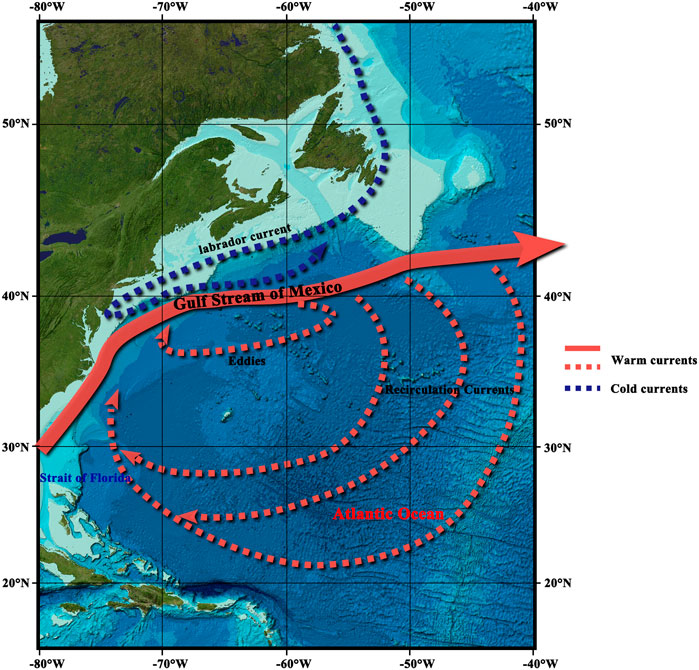
FIGURE 1. The research area and the distribution of the Gulf Stream (image is adapted from the GEBCO world map 2014, www.gebco.net).
In order to accurately separate the MDT signal from MSS and GGM, the latest MSS of CNES-CLS15MSS is introduced for modeling (Schaeffer et al., 2016; Pujol et al., 2018), where 20 years of altimetric data from 1993 to 2012 are assimilated. The CNES-CLS15MSS is represented on a 1/8° spatial resolution grid. The reference time period is 1993–2012, and the reference ellipsoid is the World Geodetic System 1984 (WGS84).
The ITSG-Grace2014s GGM (ITSG), published by the Graz University of Technology, provides full error variance-covariance information that can be conducive to the investigation of the commission error modeling (Mayer-Gürr et al., 2014). However, the ITSG is a GRACE-only GGM with a maximum expansion of d/o 200, which will be a limitation in the MDT modeling, spectrally (Table 1). In the following the ITSG model will be called the “GRACE-only GGM.” In addition, with the completion of a GOCE mission, the accuracy of GGM based on satellite-only gravimetric data has been unprecedently improved, especially in the open ocean. Therefore, the Gravity Observation Combination 06s model (GOCO06s) that provides full error variance-covariance matrix is also introduced for MDT modeling (Kvas et al., 2019b).
TABLE 1. The summary of the GGMs.
ESA has released six releases of direct GGM solutions based on GRACE/GOCE gravity data, where the fourth-release (GO_CONS_GCF_2_ DIR_R4, DIR4), the fifth-release (GO_CONS_GCF_2_DIR_R5, DIR5), and the sixth-release (GO_CONS_GCF_2_DIR_R6, DIR6) are introduced for MDT modeling. Notably, the DIR6 recalibrates the satellite orbits compared to the DIR5 (Förste et al., 2019). Besides, in order to better assess the performance of the LS-based approach in the MDT estimation, the timewise solutions that only assimilated GOCE data, including the fifth-release (GO_CONS_GCF_2_TIM_R5, TIM5) and the sixth-release (GO_CONS_GCF_2_TIM_R6, TIM6, and GO_CONS_GCF_2_TIM_R6e, TIM6e), are also introduced for MDT estimation. In the following the releases of GOCE GGM will be called the “GOCE-based GGM.” Table 1 summarizes more detailed information about these GGMs.
In addition, the XGM 2019e_2159 combined GGM (Zingerle et al., 2020), provided by Technical University of Munich, is introduced as the complementary information in the weight matrix construction in the LS-based approach. The reason for choosing XGM 2019e_2159 is that the XGM 2019e_2159 assimilated the latest Altimetry data, satellite gravity data, and ground data for modeling, which could be expanded up to 2190d/o. And comparing with the other high d/o GGMs e.g., EIGEN6c4 (Förste et al., 2014) or EGM 2008 (Pavlis et al., 2012), the XGM 2019e_2159 shows a better performance in the ocean, especially in the coastal regions (Zingerle et al., 2020).
This study introduces GOCE-based GGMs, including DIR4, DIR5/TIM5, DIR6/TIM6/TIM6e, and GOCO06s, to evaluate the contribution of GOCE-based gravimetric data for MDT modeling. Notably, all MSS and GGMs are unified to the tide-free and WGS84 reference ellipsoid.
In order to assess the performance of estimated MDT, the latest Centre National d’Etudes Spatiales - Collect Localisation Satellites 2018 Mean Dynamic Topography model (CNES-CLS18MDT, CLS18) and the Danmarks Tekniske Universitet 2017 Mean Dynamic Topography model (DTUc17MDT, DTU17) with their associated geostrophic velocity fields are introduced for comparison and validation (Knudsen et al., 2021; Mulet et al., 2021). The CLS18 utilized CNES-CLS15MSS and GOCO05S for modeling. All drifting buoy velocities and hydrological profiles from 1993 to 2017 are assimilated in CLS18 for current signal augmentation. Estimated error of the CNES-CLS18 could reach ∼10 cm around current areas and down to ∼2 cm in the other areas (Mulet et al., 2021). The DTU17 has been developed using the DTU15MSS as MSS, and EIGEN-6C4 for geoid modeling. Drifter data from 1992 to 2015 are assimilated in the DTU17, and the quasi-gaussian filter (Knudsen et al., 2021) was implemented to best fit the velocities of oceanographic drifting buoys. The estimated errors of the DTU17cMDT range from a few centimeters to a few decimeters, and they exceed 20 cm in areas of the major ocean currents (Knudsen et al., 2021). The reference period of both CLS18 and DTU17 is 1993–2012, with the spatial resolution of 1/8°. Table 2 shows more details about these two models. In this study, we take geostrophic velocity fields provided by CLS18 and DTU17 as validation data, considering that both models assimilated a large amount of in-situ data. A synthetic MDT model (Synthetic_MDT) and associated geostrophic velocity field (Synthetic_Current) were calculated from the average of the CLS18 and DTU17 for comparison and validation.
TABLE 2. | The summary of the MDT models.
The Gaussian filtered MDT will also be introduced for comparison in this study, which is derived based on a direct solution combining GGM and CNES-CLS15MSS. In this study, the same GGM information are introduced to estimated MDT and the Gaussian filtered MDT to ensure that the content between the two MDT solutions is comparable. The Gaussian filter used in this study is introduced from Jekeli (1981) and Wahr et al. (1998). The MDT values (
where
where
where
We initially set up an LS-based approach to separate MDT signal from MSS and GGM. The key point is the establishment of a complete observation equation and the associated weight matrix, which will prominently influence the separation of MDT signal from MSS and GGM. Here, we express GGM and MDT in the spatial domain, which is given as (Bingham et al., 2008)
where
where
In addition, the MDT is parameterized by the Lagrange Basis Function (LBF) (Becker et al., 2012):
where K represents the number of basis function
Due to the computer limitation, LBF with 4 parameters was used to interpolate the MDT in this study, despite the recommendation to use 16 parameters in Shi et al. (2020). MSS and GGM are extracted on a 0.5° grid, respectively, in order to reduce the correlation between the grids. For each unknown MDT point, the four points around it in the 0.5° grid are found, and a local coordinate system in this 4-points-rectangle is established. Then, the unknown MDT value in this local system is calculated based on the interpolation using LBF with 4 parameters. Finally, all the unknown MDT values can be parameterized by LBF, and the parameter coefficient matrix (
where
In this study, we investigate the use of the satellite-only GGM. In principle, SHs from d/o 2 to ∞ should be used for expression of the geoid. However, the Signal to Noise Ratio (SNR) of GGM will decrease with the increase of the expansion of GGM (Tsoulis and Patlakis, 2013; Bruinsma et al., 2014). Consequently, we segmentally construct observation equation and the weight matrix based on the error information provided by GGMs.
The expression of GGM is split into three parts and processed accordingly. The first parameters group of SHs (
In order to better extract the MDT signal from MSS and GGM, more smoothing conditions and a priori information should be added, which will be discussed in the following sub-sections.
We directly introduce SH coefficients
Here, the variance information provided in GGM (
The smoothness information should be introduced through pseudo-observation considering the SNR of GGM. Supposing that the random variables are normally distributed, the degree-wise variance function of the SH coefficients can be expressed based on Kaula’s rule (Kaula, 1966):
where
The smoothness information is introduced in
Consequently, the pseudo-observation equations can be expressed as
In the combination of MSS and GGM, the main obstruction is the limited spatial resolution of GGM. Consequently, information from
In our approach,
where
where
In order to derive a slightly smoother MDT and associated geostrophic current velocity field, additional smoothness information needs to be supplemented in the observation equation. In this study, we try to minimize the norm of the gradient of the MDT (Becker et al., 2014). The parameterization matrix of the MDT part in Eq. 8 can be expressed as
where
Hence, the smoothing information that could reduce the norm of the MDT gradient could be supplemented in observation equation by
This study expresses MSS as the combination of the MDT and the geoid, where the geoid is represented as a sum of SH functions and the associated error information provided by GGM is introduced in the modeling. The MDT is parameterized and estimated in a LS system, and observation equations are segmentally established considering the SNR of GGM. It is notable that Eq. 9 may suffer from ill-condition problem, since the SH coefficients are introduced in observation equations. Also, the estimated MDT using the LS-based approach may be coarse, due to the noises introduced from the MDT parameterization and the weight matrix. Therefore, the SH coefficients of the satellite-only GGM (Eq. 10) and the gradient term of the MDT (Eq. 19) are introduced in this study as constraints to help derive a reasonable MDT solution. In the end, the complete observation equation with its weight matrix can be expressed as
Therefore, observation equation can be solved by the weighted LS method:
where
The performance of the LS-based MDT modeling approach is evaluated in the Gulf Stream area (Figure 1). We first investigate the importance of the full variance-covariance information of GGM in the MDT modeling, where GRACE-only GGM and GOCE-based GGM are used. Then, we study the effect of gravity signal in the modeling of MDT using the latest seven releases of GOCE-based GGMs, and estimated errors of the MDT solutions will be analyzed and assessed. Effects of different choices of the cut-off frequency for
As for GRACE-only GGM (ITSG), the choice of the cut-off frequency for segmentation is
Full error variance-covariance matrix and diagonal error variance matrix from ITSG and GOCO06s are introduced in the LS system, respectively, and the corresponding solutions are compared. The MDT solutions estimated using ITSG are shown in Figure 2. Figure 2A is the Synthetic_MDT, Figures 2B–D are the Gaussian filtered MDT, the estimated MDT with full error information, and diagonal error information of GGM, respectively. Misfits between MDT solutions against the Synthetic_MDT are also illustrated in Figure 2, where Figures 2E–G are the corresponding misfits between Figures 2B–D against the Synthetic_MDT, respectively. The statistics are shown in Table 3. Notice that the land area is ignored in this experiment.
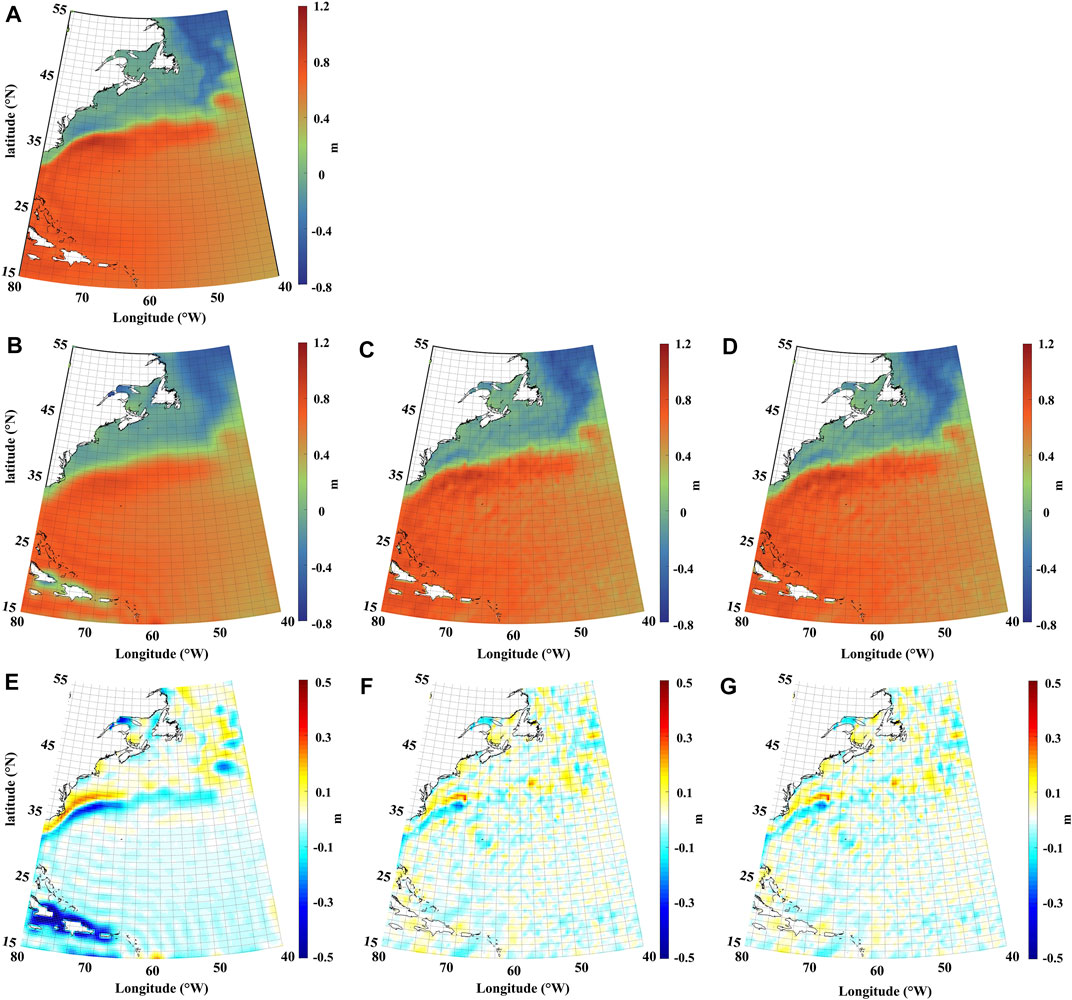
FIGURE 2. (A) the Synthetic_MDT; (B) the Gaussian filtered MDT; estimated MDT with (C) full error information, and (D) diagonal error information of GGM; and (E–G) are the corresponding misfits between (B–D) against the Synthetic_MDT, respectively.
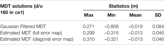
TABLE 3. Statistics of misfits between MDTs using ITSG against the Synthetic_MDT.
All MDTs provide reasonable solutions, with similar patterns of the signal distribution. Specifically, bounded by the Gulf Stream (Figure 1), the MDT in its southern part is above 0.4 m, while the MDT in the northern part is below 0.4 m. Also, it can be seen from Figure 2A, that the variation of the MDT around (38°N/70°W) is more than 1 m, and we will take it as a comparison point in this study. The MDTs derived by the two approaches could reach the level of -0.8–1.2 m in the research area. The Gaussian filtered MDT is apparently smoother than estimated MDT, while there is sharper signal in the estimated solution. The reason is that the Gaussian filter operates an isotropic spatial weighting average procedure to the signal for a smoother solution (Bingham, 2010). On the contrary, there are no additional filters introduced in estimated MDT after the LS adjustment.
As can be seen from Figures 2E–G, misfits of all three MDT solutions can reach the level of ±0.5 m. However, their distribution is different. Misfits between the Gaussian filtered MDT and the Synthetic_MDT in Figure 2E show a clear signal leakage, especially near the current and the coastal area. Specifically, the signal near current is weakened for about 0.3 m. This is because the isotropic filtering causes attenuation of the MDT gradient signal, resulting in a large discrepancy between the MDT solution and the Synthetic_MDT. The loss of the signal will have an influence not only on the model accuracy but also on further investigation in ocean currents.
In addition, Figures 3A–C show misfits between Gaussian filtered MDT, estimated MDT with full error information, and diagonal error information of GOCO06s, against the Synthetic_MDT, respectively. The statistics are shown in Table 4. Apparently, the improvement in GOCE-based MDTs is significant compared with the GRACE-only MDT, where the SD of misfits decreases from 0.046 m (ITSG) to 0.037 m (GOCO06s). It is seen from Figure 3B that there are high-frequency misfits along 38°N in the estimated MDT, but it’s apparently better suppressed comparing with that in Figure 2F using the GRACE-only GGM, which is the contribution of GOCE signal.
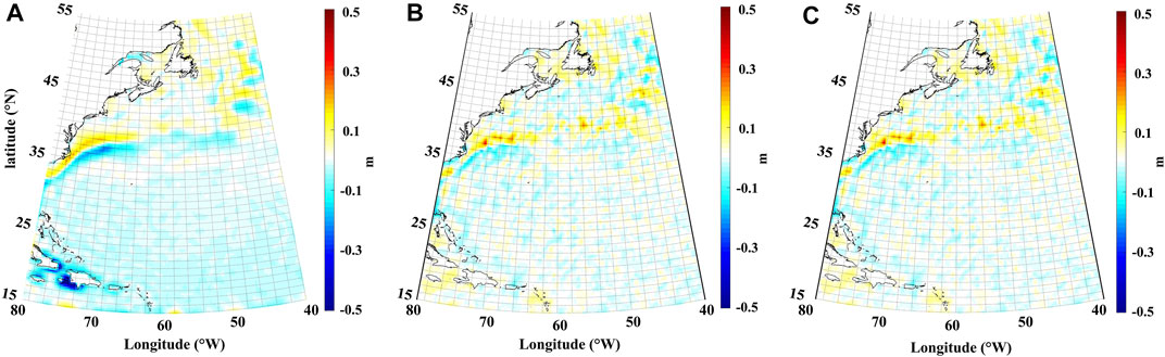
FIGURE 3. Misfits between estimated MDTs using GOCO06s against the Synthetic_MDT. [(A) Gaussian filtered MDT, (B) estimated MDT with full error information of GGM, and (C) diagonal error information of GGM, against the Synthetic_MDT. The
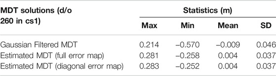
TABLE 4. Statistics of misfits between MDTs using GOCO06s against the Synthetic_MDT.
However, both results obtained from ITSG and GOCO06s show that there are only marginal differences between the MDT solutions using full error variance-covariance of GGM and using only diagonal error variance information for error modeling. Statistics show a maximum difference of 0.6 cm between these two MDT solutions, with a SD of ∼0.05 cm. This is likely because the diagonal elements of SHs coefficients play a major role in GGM signal (Gruber, 2001; Ran et al., 2021). Consequently, only the diagonal error variance information of GGM will be considered in the following MDT modeling using GOCE-based GGM in the next section.
Comparing with the Synthetic_MDT, both the Gaussian filtered solution and estimated MDT solution will show signal attenuation near the current. For example, alternating positive and negative misfits are seen around 30°N–38°N, which is induced by the over-smooth in the Gaussian filtering or the smoothness condition in the LS system. The estimated MDT recovers more signal than the Gaussian filtered one. Misfits of the estimated MDTs (Figures 2F, 3B) around 30–38°N are significantly smaller compared with the Gaussian filtered solution (Figures 2E, 3A). Statistics in Tables 3, 4 show that, although the SD of misfits between Gaussian filtered MDT and the Synthetic_MDT decreases from 0.084 m (ITSG) to 0.046 m (GOCO06s), the MDT estimated by the LS-based approach are still a better fit with the Synthetic_MDT. The SD of misfits between the estimated MDTs and the Synthetic_MDT decreases from 0.046 m (ITSG) to 0.037 m (GOCO06s). In addition, the signals around the coast in the southwestern part of the research area are better recovered than the Gaussian filtered solution, indicating the superiority of the LS-based approach in the MDT modeling.
In order to further assess the performance of GOCE-based GGMs in MDT estimation, seven GOCE-based GGMs (i.e., DIR4, DIR5/TIM5, DIR6/TIM6/TIM6e, and GOCO06s) are investigated, and their MDT solutions are compared. The strategies for MDT modeling are the same as in Section 4.1. Considering the SNR of the GGMs, the cut-off frequency for
Figure 4 shows misfits between the MDT solutions using (A) Gaussian filtering, (B) DIR4, (C) DIR5, (D) TIM5, (E) DIR6, (F) TIM6, (G) TIM6e, and (H) GOCO06S, against the Synthetic_MDT, respectively. The statistics of misfits between the estimated MDT and the Synthetic_MDT are shown in Table 5. The Gaussian filtered MDT still suffers from the severe signal leakage problem near the current and coast region in the southwestern part of the research area. For instance, misfit around 38°N/70°W is ∼±0.1 m in the estimated solutions, while it increases to ∼±0.2 m in the Gaussian filtered solution. The statistics in Table 5 show that the SD of misfits of the MDT solutions using DIR4, DIR5/TIM5, DIR6/TIM6/TIM6e, and GOCO06s is 0.039, 0.038/0.040, 0.036/0.038/0.038, and 0.037 m, respectively. The SD of misfits of the Gaussian filtered MDT increases to 0.041 m. The statistics of misfits show that the estimated MDT using GOCO06s and DIR6 perform the best in this study. However, the MDT based on DIR6 only shows 0.3 cm better agreement with the Synthetic_MDT than that based on DIR4. Besides, when comparing with the same release of the GGM, the estimated MDT using direct GGM solution shows better performance than the timewise GGM solution. For example, the SD of misfits of the estimated MDT using TIM6 show ∼0.2 cm larger than the MDT using DIR6. Estimated errors are deduced based on the error propagation using DIR6, shown in Figure 5, where
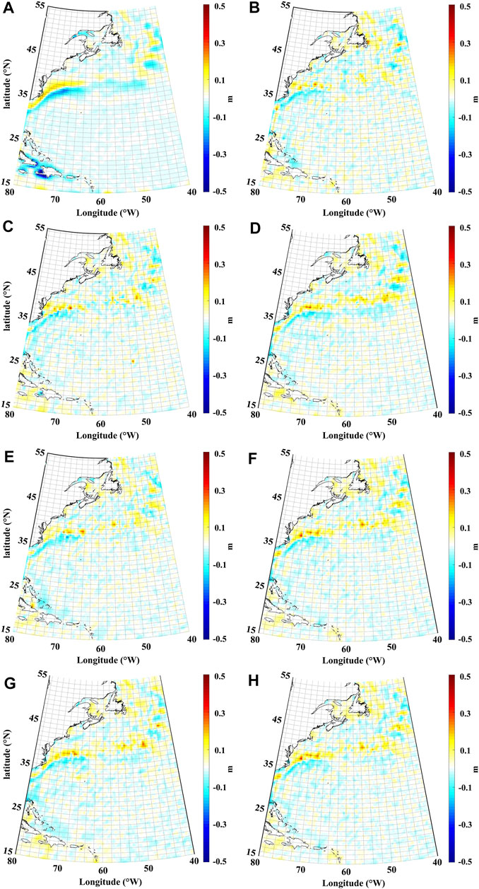
FIGURE 4. Misfits between estimated MDTs against the Synthetic_MDT. (The MDT solutions using (A) Gaussian filtering, (B) DIR4, (C) DIR5, (D) TIM5, (E) DIR6, (F) TIM6, (G) TIM6e, and (H) GOCO06s, against the Synthetic_MDT, respectively. The
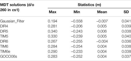
TABLE 5. Statistics of misfits between GOCE-based MDTs against the Synthetic_MDT.
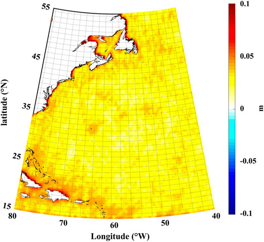
FIGURE 5. Estimated errors based on DIR6 with
Further, the effect of different choices of the cut-off frequency for
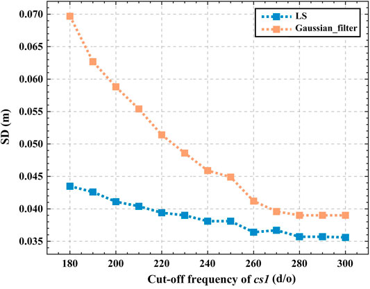
FIGURE 6. The SD of misfits under different cut-off frequency of
Geostrophic current velocities are calculated based on estimated MDT and the Gaussian filtered MDT, where DIR6 in d/o 260 is used in the calculation. The MDT signal may be smoothed out from the coast or current, and into the surrounding ocean due to filtering, causing current signal attenuation. Accordingly, it is necessary to utilize geostrophic current data for validating deduced geostrophic current using estimated MDT and the Gaussian filtered MDT. Geostrophic current velocities can be given as (Lagerloef et al., 1999):
where u and v denote the eastward and the northward component of geostrophic current velocity, respectively.
In the top panel of Figure 7, estimated geostrophic currents deduced from different MDT solutions are illustrated, where Figures 7A–C represent the geostrophic current derived from Synthetic_Current, estimated MDT, and Gaussian filtered MDT, respectively. And in the bottom panel of Figure 7, misfits between deduced geostrophic current against the Synthetic_Current are illustrated, where Figures 7D,E represent misfits from the estimated MDT (DIR6) and Gaussian filtered MDT, respectively. The Synthetic_Current can reach the level of 0.5–1.0 m/s in the research area, while results obtained from estimated MDT and Gaussian filtered MDT in Figures 7B,C are weaker by 0.3–0.5 m/s. There are two main reasons for this signal attenuation. First, geostrophic velocity information from Synthetic_Current assimilated a large number of in-situ measurements to enhance the current signal in the model. In addition, the expansion of GGM and the imposed spatial filtering or smoothing condition will make an attenuation of geostrophic current signal. It is notable that the signal of geostrophic current in the open ocean in Figure 7B is relatively larger compared to Figures 7A,C. The main reason is that the MDT estimated using the LS-based approach is still not as smooth as the Gaussian filtered MDT, so the geostrophic current signal is amplified where the gradient of the MDT is overestimated.
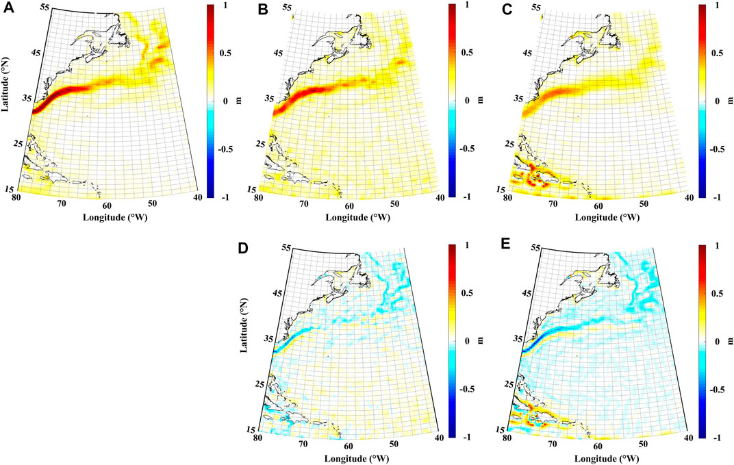
FIGURE 7. Top panel: Estimated geostrophic currents deduced from (A) Synthetic_Current, (B) estimated MDT, and (C) Gaussian filtered MDT are illustrated, respectively. Bottom panel: misfits between deduced geostrophic current against the Synthetic_Current, where the misfits from (D) estimated MDT (DIR6) and (E) Gaussian filtered MDT are illustrated, respectively.
It is seen from the bottom panel of Figure 7 that both deduced geostrophic current fields are relatively weaker than the Synthetic_Current. For instance, geostrophic current velocities derived by the Gaussian filtering approach show significant misfits in the coast of the Gulf Stream. However, by comparing Figures 7D,E, it can be seen that the signal attenuation problem in geostrophic current obtained by the LS-based approach is better suppressed, where misfits are smaller. More importantly, the deduced geostrophic current velocities using Gaussian filtered MDT shows stronger noise signal in the coastal area in the southwestern part of the research area, indicating a signal distortion problem. Estimated MDT recovers better geostrophic current velocities in both the coastal and current regions than the Gaussian filtered MDT. Table 6 shows the statistics of misfits between geostrophic current obtained from the LS-based approach and Gaussian filtering, against the Synthetic_Current. It can be seen that the SD of misfits of geostrophic currents derived by the LS-based approach is 0.062 m/s, which shows 1.8 cm/s better agreement than the Gaussian filtered MDT.
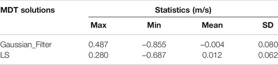
TABLE 6. Statistics of misfits between geostrophic current against the Synthetic_Current.
The traditional geodetic MDT modeling approach requires a filter procedure in the spatial or spectral domain to derive a reasonable solution, which inevitably lead to signal attenuation problems. In this study, we focus on using an LS-based approach for MDT modeling to limit the usage of spatial filtering. This approach constructs observation equations segmentally and carefully models the power matrices of each spectral domain. Further, the unknown parameters of the MDT are estimated in the LS system. Satellite-only GGMs including GRACE-only GGM and seven GOCE-based GGMs with error information are used for MDT modeling, where the effects of the error variance-covariance information from GGM and the contribution of the geoid signal in
Results show that applications of full error variance-covariance matrix or only diagonal error variance of GGMs may have marginal effects on the MDT modeling. The latest GOCE-based GGMs, i.e., DIR6 and GOCO06s, reveal the best geodetic MDT solution using the LS-based approach, where the SD of the MDT misfits is 0.036 and 0.037 m if d/o 260. The estimated error map based on the error propagation illustrates that errors are more concentrated near the coastal region (∼0.1 m in Figure 5), while it reduces to ∼0.05 m (Figure 5) in the open ocean. The validation using deduced geostrophic velocities shows that estimated MDT recovers better geostrophic current signal in both the coastal and current region than the Gaussian filtered MDT. The SD of geostrophic current misfits by estimated MDT shows an improvement by 1.8 cm/s, comparing with the corresponding ones estimated by the Gaussian filtered MDT.
More future work need to be done to further assess and improve the LS-based MDT modeling approach. First, in order to study the variation of ocean currents due to the global sea level rise over the years, it is necessary to adjust the reference time of the MSS to the last 20 years (e.g., 1997–2018). It is notable that the MDT solutions derived in this study are referenced to the time period 1993–2012. However, with the study of the accumulated altimetry data, it is found that the sea level is rising gradually due to global warming (Hamlington et al., 2020), which will significantly affect the MDT and deduced geostrophic current. Research reveals that there is more prominent sea state variation near ocean current. For example, Gonçalves Neto et al. (2021) showed that the MSS in the Gulf Stream increased by an average of 4.5 cm from 2009 to 2018 compared to 1993–2007, and there is a significant increase (up to 15 cm) in the northern part of the Gulf Stream and a decrease of up to 15 cm in the southern part of the Gulf Stream. This means that the Gulf Stream is moving to the north. Therefore, the MDT and geostrophic current signal referenced to the last 20 years needs to be further investigated. Second, it is important to use independent in-situ data for robust validation of MDT solutions. For example, the drift data from the Argo program should be reprocessed and used as validation data. And in order to facilitate studies on the vertical datum unification, the performance of the estimated MDT in the coastal region needs to be evaluated using tide gauges. What’s more, a comprehensive comparison and analysis of several up-to-date MDT modeling methods, e.g., Andersen et al. (2018a), Karimi et al. (2020), and Wu et al. (2021), together with the LS-based approach need to be performed, and their performance near current and coast region should be further investigated. In this study, the spatial resolution of the MDT is lower than that of DTU15MDT/CNES-CLS18MDT due to the computation limitation of the global SHs. One solution is to replace SHs with a radial basis function (Wu et al., 2018), which could reduce the size of the design matrix and save the computation resources. It is also necessary to evaluate the error information of the altimetric data and introduce altimetric data into the LS system for the MDT modeling.
The raw data supporting the conclusion of this article will be made available by the authors, without undue reservation.
HS designed this research, carried out experiments and data analysis, visualized the figures and drafted the manuscript. YW, OA, and PK conceived and coordinated this research. XH and YL participated in research coordination. ZZ participated in figure visualization. All the seven authors contributed to discuss results and reviewed the manuscript.
The project was funded by the National Natural Science Foundation of China (Nos. 41830110, 42004008, 42004014), the Postgraduate Research and Practice Innovation Program of Jiangsu Province (KYCX21_0530), the Fundamental Research Funds for the Central Universities, the Guangxi Key Laboratory of Spatial Information and Geomatics (NO. 19-185-10-06), the Natural Science Foundation of Jiangsu Province, China (Nos. BK20190498, BK20200530), the National Key Research Development Program of China (No. 2018YFC1503603), Foundation for Returned Overseas Chinese Scholars, Nanjing (No. B2004804), the State Scholarship Fund from Chinese Scholarship Council (Nos. 202006710169, 201306270014).
The authors declare that the research was conducted in the absence of any commercial or financial relationships that could be construed as a potential conflict of interest.
All claims expressed in this article are solely those of the authors and do not necessarily represent those of their affiliated organizations, or those of the publisher, the editors, and the reviewers. Any product that may be evaluated in this article, or claim that may be made by its manufacturer, is not guaranteed or endorsed by the publisher.
The authors would like to thank DTU space and CNES/CLS for providing the DTU17cMDT and CNES-CLS15MSS/CNES-CLS18MDT products. The authors would also like to thank the ICEGM, the Graz University of Technology and ESA for providing ITSG and releases of GOCE GGM. The authors would like to give sincerest thanks to the reviewers for their beneficial suggestions and comments, which are of great value for improving the manuscript. The authors also thank the Editor ME for the kind assistance and constructive comments.
The Supplementary Material for this article can be found online at: https://www.frontiersin.org/articles/10.3389/feart.2022.795935/full#supplementary-material
Andersen, O. B., and Knudsen, P. (2009). DNSC08 Mean Sea Surface and Mean Dynamic Topography Models. J. Geophys. Res. 114, C11001. doi:10.1029/2008jc005179
Andersen, O. B., Nielsen, K., Knudsen, P., Hughes, C. W., Bingham, R., Fenoglio-Marc, L., et al. (2018a). Improving the Coastal Mean Dynamic Topography by Geodetic Combination of Tide Gauge and Satellite Altimetry. Mar. Geodesy 41, 517–545. doi:10.1080/01490419.2018.1530320
Andersen, O. B., Rose, S. K., Knudsen, P., and Stenseng, L. (2018b). “The DTU18 MSS Mean Sea Surface Improvement from SAR Altimetry,” in Proceedings of the 25 years of progress in radar altimetry symposium, 24–29 September, Portugal, 24–26.
Bai, X., Yan, H., Zhu, Y., Peng, P., Yan, Y., and Shen, Y. (2020). Formal Error Assessment of Geodetic Mean Dynamic Topography at Different Spatial Scales. J. Geodynamics 138, 101753. doi:10.1016/j.jog.2020.101753
Barthelmes, F. (2013). Definition of Functionals of the Geopotential and Their Calculation from Spherical Harmonic Models: Theory and Formulas Used by the Calculation Service of the International Centre for Global Earth Models (ICGEM). Potsdam: Deutsches GeoForschungsZentrum GFZ. Scientific Technical Report. ISSN 1610-0956, Potsdam, Germany. doi:10.2312/gfz.b103-0902-26
Baur, O., and Grafarend, E. W. (2006). “High-Performance GOCE Gravity Field Recovery from Gravity Gradient Tensor Invariants and Kinematic Orbit Information,” in Observation of the Earth System from Space. Editors J. Flury, R. Rummel, C. Reigber, M. Rothacher, G. Boedecker, and U. Schreiber (Berlin/Heidelberg: Springer-Verlag), 239–253. doi:10.1007/3-540-29522-4_17
Becker, S., Brockmann, J. M., and Schuh, W.-D. (2014). Mean Dynamic Topography Estimates Purely Based on GOCE Gravity Field Models and Altimetry. Geophys. Res. Lett. 41, 2063–2069. doi:10.1002/2014gl059510
Becker, S., Freiwald, G., Losch, M., and Schuh, W.-D. (2012). Rigorous Fusion of Gravity Field, Altimetry and Stationary Ocean Models. J. Geodynamics 59-60 (60), 99–110. doi:10.1016/j.jog.2011.07.006
Bingham, R. J., Haines, K., and Hughes, C. W. (2008). Calculating the Ocean's Mean Dynamic Topography from a Mean Sea Surface and a Geoid. J. Atmos. Oceanic Tech. 25, 1808–1822. doi:10.1175/2008jtecho568.1
Bingham, R. J., Haines, K., and Lea, D. J. (2014). How Well Can We Measure the Ocean's Mean Dynamic Topography from Space? J. Geophys. Res. Oceans 119, 3336–3356. doi:10.1002/2013jc009354
Bingham, R. J. (2010). Nonlinear Anisotropic Diffusive Filtering Applied to the Ocean's Mean Dynamic Topography. Remote Sensing Lett. 1, 205–212. doi:10.1080/01431161003743165
Bock, H., Jäggi, A., Beutler, G., and Meyer, U. (2014). GOCE: Precise Orbit Determination for the Entire mission. J. Geod 88, 1047–1060. doi:10.1007/s00190-014-0742-8
Brockmann, J. M. (2014). On High Performance Computing in Geodesy : Applications in Global Gravity Field Determination. Dissertation. Bonn: Rheinische Friedrich-Wilhelms-Universität Bonn. Available at: https://nbn-resolving.org/urn:nbn:de:hbz:5n-38608.
Bruinsma, S. L., Förste, C., Abrikosov, O., Lemoine, J.-M., Marty, J.-C., Mulet, S., et al. (2014). ESA's Satellite-Only Gravity Field Model via the Direct Approach Based on All GOCE Data. Geophys. Res. Lett. 41, 7508–7514. doi:10.1002/2014GL062045
Chambers, D., Andersen, O. B., Rio, M.-H., Rummel, R., Wiese, D., et al. (2017). “Auxiliary Space-Based Systems for Interpreting Satellite Altimetry,” in Satellite Altimetry Over Oceans And Land Surfaces. Editors D. Stammer, and A. Cazenave (Boca Raton, FLTaylor & Francis: CRC Press), 149–186. doi:10.1201/9781315151779-4
Donlon, C. J., Cullen, R., Giulicchi, L., Vuilleumier, P., Francis, C. R., Kuschnerus, M., et al. (2021). The Copernicus Sentinel-6 Mission: Enhanced Continuity of Satellite Sea Level Measurements from Space. Remote Sensing Environ. 258, 112395. doi:10.1016/j.rse.2021.112395
Drinkwater, M. R., Floberghagen, R., Haagmans, R., Muzi, D., and Popescu, A. (2003). “GOCE: ESA's First Earth Explorer Core Mission,” in Earth Gravity Field From Space — From Sensors To Earth Sciences Space Sciences Series of ISSI. Editors G. Beutler, M. R. Drinkwater, R. Rummel, and R. Von Steiger (Dordrecht: Springer Netherlands), 419–432. doi:10.1007/978-94-017-1333-7_36
Flechtner, F., Morton, P., Watkins, M., and Webb, F. (2014). “Status of the GRACE Follow-On Mission,” in Gravity, Geoid And Height Systems International Association of Geodesy Symposia. Editor U. Marti (Cham: Springer International Publishing), 117–121. doi:10.1007/978-3-319-10837-7_15
Förste, C., Abrykosov, O., Bruinsma, S., Dahle, C., König, R., and Lemoine, J.-M. (2019). ESA’s Release 6 GOCE Gravity Field Model by Means of the Direct Approach Based on Improved Filtering of the Reprocessed Gradients of the Entire mission (GO_CONS_GCF_2_DIR_R6). 3 Files. Potsdam, Germany: GFZ Data Services. doi:10.5880/ICGEM.2019.004
Förste, C., Bruinsma, S., Abrikosov, O., Flechtner, F., Marty, J. C., Lemoine, J. M., et al. (2014). EIGEN-6C4-The Latest Combined Global Gravity Field Model Including GOCE Data up to Degree and Order 1949 of GFZ Potsdam and GRGS Toulouse. EGU Gen. Assembly Conf. Abstr. 16, 3707. doi:10.5880/icgem.2015.1
Freiwald, G. (2013). A New Filter for the Mean Dynamic Topography of the Ocean Derived Directly from Satellite Observations. J. Geodynamics 72, 67–71. doi:10.1016/j.jog.2013.08.006
Gonçalves Neto, A., Langan, J. A., and Palter, J. B. (2021). Changes in the Gulf Stream Preceded Rapid Warming of the Northwest Atlantic Shelf. Commun. Earth Environ. 2, 74. doi:10.1038/s43247-021-00143-5
Gruber, T. (2001). High-Resolution Gravity Field Modeling with Full Variance-Covariance Matrices. J. Geodesy 75, 505–514. doi:10.1007/s001900100202
Hamlington, B. D., Gardner, A. S., Ivins, E., Lenaerts, J. T. M., Reager, J. T., Trossman, D. S., et al. (2020). Understanding of Contemporary Regional Sea‐Level Change and the Implications for the Future. Rev. Geophys. 58, e2019RG000672. doi:10.1029/2019RG000672
Haynsworth, E. V. (1968). On the Schur Complement. Base1 Mathematical Notes, BMN 20, Basel: University of Basel.
Hwang, C., Hsu, H.-Y., and Jang, R.-J. (2002). Global Mean Sea Surface and marine Gravity Anomaly from Multi-Satellite Altimetry: Applications of Deflection-Geoid and Inverse Vening Meinesz Formulae. J. Geodesy 76, 407–418. doi:10.1007/s00190-002-0265-6
Jekeli, C. (1981). Alternative Methods to Smooth the Earth’s Gravity Field. Columbus: Department of Geodetic Science and Surveying, Ohio State University.
Kang, D., and Curchitser, E. N. (2013). Gulf Stream Eddy Characteristics in a High-Resolution Ocean Model. J. Geophys. Res. Oceans 118, 4474–4487. doi:10.1002/jgrc.20318
Karimi, A. A., Andersen, O. B., and Deng, X. (2021). Mean Sea Surface and Mean Dynamic Topography Determination from Cryosat-2 Data Around Australia. Adv. Space Res. 68 (2), 1073–1089. doi:10.1016/j.asr.2020.01.009
Ke, B., Zhang, L., Xu, J., Zhang, C., and Dang, Y. (2019). Determination of the Mean Dynamic Ocean Topography Model through Combining Multi-Source Gravity Data and DTU15 MSS Around China's Coast. Adv. Space Res. 63, 203–212. doi:10.1016/j.asr.2018.10.040
Klymak, J. M., Shearman, R. K., Gula, J., Lee, C. M., D'Asaro, E. A., Thomas, L. N., et al. (2016). Submesoscale Streamers Exchange Water on the North Wall of the Gulf Stream. Geophys. Res. Lett. 43, 1226–1233. doi:10.1002/2015GL067152
Knudsen, P., Andersen, O., and Maximenko, N. (2021). A New Ocean Mean Dynamic Topography Model, Derived from a Combination of Gravity, Altimetry and Drifter Velocity Data. Adv. Space Res. 68, 1090–1102. doi:10.1016/j.asr.2019.12.001
Knudsen, P., Bingham, R., Andersen, O., and Rio, M.-H. (2011). A Global Mean Dynamic Topography and Ocean Circulation Estimation Using a Preliminary GOCE Gravity Model. J. Geod 85, 861–879. doi:10.1007/s00190-011-0485-8
Kvas, A., Behzadpour, S., Ellmer, M., Klinger, B., Strasser, S., Zehentner, N., et al. (2019a). ITSG‐Grace2018: Overview and Evaluation of a New GRACE‐Only Gravity Field Time Series. J. Geophys. Res. Solid Earth 124, 9332–9344. doi:10.1029/2019JB017415
Kvas, A., Mayer-Gürr, T., Krauss, S., Brockmann, J. M., Schubert, T., Schuh, W. D., et al. (2019b). The Satellite-Only Gravity Field Model GOCO06s. Potsdam, Germany: GFZ Data Services. doi:10.5880/ICGEM.2019.002
Lagerloef, G. S. E., Mitchum, G. T., Lukas, R. B., and Niiler, P. P. (1999). Tropical Pacific Near-Surface Currents Estimated from Altimeter, Wind, and Drifter Data. J. Geophys. Res. 104, 23313–23326. doi:10.1029/1999jc900197
Landerer, F. W., Flechtner, F. M., Save, H., Webb, F. H., Bandikova, T., Bertiger, W. I., et al. (2020). Extending the Global Mass Change Data Record: GRACE Follow‐On Instrument and Science Data Performance. Geophys. Res. Lett. 47, e2020GL088306. doi:10.1029/2020GL088306
Lawson, C. L., and Hanson, R. J. (1995). Solving Least Squares Problems. Newyork: Society for Industrial and Applied Mathematics.
Le Traon, P.-Y., Antoine, D., Bentamy, A., Bonekamp, H., Breivik, L. A., Chapron, B., et al. (2015). Use of Satellite Observations for Operational Oceanography: Recent Achievements and Future Prospects. J. Oper. Oceanography 8, s12–s27. doi:10.1080/1755876x.2015.1022050
Mayer-Gürr, T., Norbert, Z., Beate, K., and Andreas, K. (2014). “ITSG-Grace2014: A New GRACE Gravity Field Release Computed in Graz,” in Presented at: Grace Science Team Meeting 2014, Potsdam, Germany, 28-30 September. doi:10.13140/rg.2.1.5098.2805
Mulet, S., Rio, M.-H., Etienne, H., Artana, C., Cancet, M., Dibarboure, G., et al. (2021). The New CNES-CLS18 Global Mean Dynamic Topography. Ocean Sci. 13, 789–808. doi:10.5194/os-2020-117
Pail, R., Goiginger, H., Schuh, W.-D., Höck, E., Brockmann, J. M., Fecher, T., et al. (2010). Combined Satellite Gravity Field modelGOCO01Sderived from GOCE and GRACE. Geophys. Res. Lett. 37, L20314. doi:10.1029/2010GL044906
Palter, J. B. (2015). The Role of the Gulf Stream in European Climate. Annu. Rev. Mar. Sci. 7, 113–137. doi:10.1146/annurev-marine-010814-015656
Pavlis, N. K., Holmes, S. A., Kenyon, S. C., and Factor, J. K. (2012). The Development and Evaluation of the Earth Gravitational Model 2008 (EGM2008). J. Geophys. Res. 117, a–n. doi:10.1029/2011jb008916
Pujol, M. I., Schaeffer, P., Faugère, Y., Raynal, M., Dibarboure, G., and Picot, N. (2018). Gauging the Improvement of Recent Mean Sea Surface Models: A New Approach for Identifying and Quantifying Their Errors. J. Geophys. Res. Oceans 123, 5889–5911. doi:10.1029/2017jc013503
Ran, J., Tangdamrongsub, N., and Wan, X. (2021). The Impact of Error Covariance Matrix Structure of GRACE's Gravity Solution on the Mass Flux Estimates of Greenland Ice Sheet. Adv. Space Res. 67, 163–178. doi:10.1016/j.asr.2020.07.012
Rio, M.-H. (2004). A Mean Dynamic Topography Computed over the World Ocean from Altimetry, In Situ Measurements, and a Geoid Model. J. Geophys. Res. 109, C12032. doi:10.1029/2003jc002226
Rio, M.-H., Pascual, A., Poulain, P.-M., Menna, M., Barceló, B., and Tintoré, J. (2014). Computation of a New Mean Dynamic Topography for the Mediterranean Sea from Model Outputs, Altimeter Measurements and Oceanographic In Situ Data. Ocean Sci. 10, 731–744. doi:10.5194/os-10-731-2014
Rio, M. H., Guinehut, S., and Larnicol, G. (2011). New CNES‐CLS09 Global Mean Dynamic Topography Computed from the Combination of GRACE Data, Altimetry, and In Situ Measurements. J. Geophys. Res. 116, C07018. doi:10.1029/2010jc006505
Rossby, T., Flagg, C., and Donohue, K. (2010). On the Variability of Gulf Stream Transport from Seasonal to Decadal Timescales. J Mar. Res. 68, 503–522. doi:10.1357/002224010794657128
Sánchez-Reales, J. M., Andersen, O. B., and Vigo, M. I. (2016). Improving Surface Geostrophic Current from a GOCE-Derived Mean Dynamic Topography Using Edge-Enhancing Diffusion Filtering. Pure Appl. Geophys. 173, 871–884. doi:10.1007/s00024-015-1050-9
Schaeffer, P., Pujol, I., Faugere, Y., Guillot, A., and Picot, N. (2016). The CNES CLS 2015 Global Mean Sea Surface. Available at: http://meetings.aviso.altimetry.fr/fileadmin/user_upload/tx_ausyclsseminar/files/GEO_03_Pres_OSTST2016_MSS_CNES_CLS2015_V1_16h55.pdf (Accessed January 25, 2022).
Shi, H., He, X., Wu, Y., and Huang, J. (2020). The Parameterization of Mean Dynamic Topography Based on the Lagrange Basis Functions. Adv. Space Res. 66, 2122–2140. doi:10.1016/j.asr.2020.07.042
Siegismund, F. (2020). A Spectrally Consistent Globally Defined Geodetic Mean Dynamic Ocean Topography. J. Geophys. Res. Oceans 125, e2019JC016031. doi:10.1029/2019jc016031
Swenson, S., and Wahr, J. (2002). Methods for Inferring Regional Surface-Mass Anomalies from Gravity Recovery and Climate Experiment (GRACE) Measurements of Time-Variable Gravity. J. Geophys. Res. 107, 3–1. doi:10.1029/2001JB000576
Tapley, B. D., Bettadpur, S., Watkins, M., and Reigber, C. (2004). The Gravity Recovery and Climate experiment: Mission Overview and Early Results. Geophys. Res. Lett. 31, 4. doi:10.1029/2004GL019920
Tapley, B. D., Chambers, D. P., Bettadpur, S., and Ries, J. C. (2003). Large Scale Ocean Circulation from the GRACE GGM01 Geoid. Geophys. Res. Lett. 30, L018622. doi:10.1029/2003GL018622
Tsoulis, D., and Patlakis, K. (2013). A Spectral Assessment Review of Current Satellite-Only and Combined Earth Gravity Models. Rev. Geophys. 51, 186–243. doi:10.1002/rog.20012
Tziavos, I. N., Vergos, G. S., Grigoriadis, V. N., Tzanou, E. A., and Natsiopoulos, D. A. (2015). “Validation of GOCE/GRACE Satellite Only and Combined Global Geopotential Models over Greece in the Frame of the GOCESeaComb Project,” in IAG 150 Years International Association Of Geodesy Symposia. Editors C. Rizos, and P. Willis (Cham: Springer International Publishing), 297–304. doi:10.1007/1345_2015_160
Vianna, M. L., Menezes, V. V., and Chambers, D. P. (2007). A High Resolution Satellite-Only GRACE-Based Mean Dynamic Topography of the South Atlantic Ocean. Geophys. Res. Lett. 34, L24604. doi:10.1029/2007GL031912
Vignudelli, S., Birol, F., Benveniste, J., Fu, L.-L., Picot, N., Raynal, M., et al. (2019). Satellite Altimetry Measurements of Sea Level in the Coastal Zone. Surv. Geophys. 40, 1319–1349. doi:10.1007/s10712-019-09569-1
Wahr, J., Molenaar, M., and Bryan, F. (1998). Time Variability of the Earth's Gravity Field: Hydrological and Oceanic Effects and Their Possible Detection Using GRACE. J. Geophys. Res. 103, 30205–30229. doi:10.1029/98JB02844
Woodworth, P. L., Gravelle, M., Marcos, M., Wöppelmann, G., and Hughes, C. W. (2015). The Status of Measurement of the Mediterranean Mean Dynamic Topography by Geodetic Techniques. J. Geod 89, 811–827. doi:10.1007/s00190-015-0817-1
Wu, Y., Huang, J., Shi, H., and He, X. (2021). Mean Dynamic Topography Modeling Based on Optimal Interpolation from Satellite Gravimetry and Altimetry Data. Appl. Sci. 11, 5286. doi:10.3390/app11115286
Wu, Y., Luo, Z., Zhong, B., and Xu, C. (2018). A Multilayer Approach and its Application to Model a Local Gravimetric Quasi-Geoid Model over the North Sea: QGNSea V1.0. Geosci. Model. Dev. 11, 4797–4815. doi:10.5194/gmd-11-4797-2018
Wu, Y., Zhou, H., Zhong, B., and Luo, Z. (2017). Regional Gravity Field Recovery Using the GOCE Gravity Gradient Tensor and Heterogeneous Gravimetry and Altimetry Data. J. Geophys. Res. Solid Earth 122, 6928–6952. doi:10.1002/2017jb014196
Keywords: mean dynamic topography, geostrophic current, signal reconstruction, Gulf stream, mean sea surface, global geopotential model, least squares
Citation: Shi H, He X, Wu Y, Andersen OB, Knudsen P, Liu Y and Zhang Z (2022) Spectrally Consistent Mean Dynamic Topography by Combining Mean Sea Surface and Global Geopotential Model Through a Least Squares-Based Approach. Front. Earth Sci. 10:795935. doi: 10.3389/feart.2022.795935
Received: 15 October 2021; Accepted: 03 January 2022;
Published: 16 February 2022.
Edited by:
Mehdi Eshagh, University West, SwedenReviewed by:
Jinyun Guo, Shandong University of Science and Technology, ChinaCopyright © 2022 Shi, He, Wu, Andersen, Knudsen, Liu and Zhang. This is an open-access article distributed under the terms of the Creative Commons Attribution License (CC BY). The use, distribution or reproduction in other forums is permitted, provided the original author(s) and the copyright owner(s) are credited and that the original publication in this journal is cited, in accordance with accepted academic practice. No use, distribution or reproduction is permitted which does not comply with these terms.
*Correspondence: Xiufeng He, eGZoZUBoaHUuZWR1LmNu; Yihao Wu, eWloYW93dUBoaHUuZWR1LmNu
Disclaimer: All claims expressed in this article are solely those of the authors and do not necessarily represent those of their affiliated organizations, or those of the publisher, the editors and the reviewers. Any product that may be evaluated in this article or claim that may be made by its manufacturer is not guaranteed or endorsed by the publisher.
Research integrity at Frontiers
Learn more about the work of our research integrity team to safeguard the quality of each article we publish.