A Data-Based Minimal Model of Episodic Inflation Events at Volcanoes

Space geodetic time series, be they ground-based or space-based, have increased in length and accuracy. These series can now be mined for information on the qualitative dynamics of volcanic systems directly from surface deformation data. Here, we study three volcanoes: Akutan and Okmok that are part of the Aleutian arc, and Piton de la Fournaise on la Reunion Island. All three are continuously monitored by the Global Positioning System (GPS) and exhibit common stair step–shaped inflation cycles sometimes referred to as to as “episodic inflation events”. Here we seek to characterize the corresponding dynamical regime of pressure build-up within their plumbing system. To do so, we make use of Multichannel Singular Spectrum Analysis (M-SSA), a data-adaptive, non-parametric time series analysis methodology that allows for 1) the reliable detection and extraction of such patterns even when the corresponding signal lies close to, or even below, the data scatter; and 2) the extraction of information relevant to the underlying qualitative dynamics without a priori assumptions on the underlying physical mechanisms. For our three volcanoes, we find that the inflation cycles resemble the relaxation oscillations of a simple oscillator that involves a nonlinear dissipative mechanism. This finding provides important guidelines for physics-based models of episodic inflation cycles. In fact, the three volcanoes share a plumbing system composed of several interconnected storage bodies. Guided by the qualitative M-SSA–inferred dynamics, we formulate a simple physical model of two magma bodies connected by a conduit in which the viscosity of the fluid varies with temperature or magma crystallization. We show that such a model possesses internal relaxation oscillations similar to those of a simple oscillator. These oscillations correspond to repetitive events with sharp variations in the rate of magma transport and they can account for episodic events of pressure build-up in magma bodies, with no need for a time-dependent magma flux into or out of the system. We also show that the model’s number of degrees of freedom is consistent with the amount of information extracted from M-SSA data analysis. The approach presented here relies on the robust statistical analysis of deformation time series to constrain the phenomenology of pressure build-up within a volcanic plumbing system; it provides a novel framework for understanding the dynamics of volcanic systems.

1 Introduction and Motivation

A large, and rapidly increasing, volume of continuous space geodetic observations is now available from ground-based data using the Global Positioning System (GPS) or from space-based data using Interferometric Satellite Aperture Radar (InSAR). These data sets are particularly dense in areas of volcanic unrest and they show a range of nonlinear temporal evolutions of surface deformation that reflect the dynamics of the underlying magmatic processes and provide information on the way pressure builds up within plumbing systems (Biggs and Pritchard, 2017). These processes may include magma flux into the magmatic plumbing system or out of it (Dvorak and Okamura, 1987; Mériaux and Jaupart, 1995; Parks et al., 2012), crystallization and degassing in melt reservoirs (Tait et al., 1989; Caricchi et al., 2014; Degruyter and Huber, 2014) or hydrothermal circulation driven by the magmatic thermal anomaly (Lu et al., 2010; Hutchison et al., 2016). The resulting surface deformation is sometimes readily visible from geodetic time series (Newman et al., 2006; Feng and Newman, 2009). In other cases, advanced time series analysis techniques have shown that nonlinear deformation caused by magmatic processes can be present during seemingly quiet time intervals where little or no deformation is apparent in the data (Ji and Herring, 2011; Walwer et al., 2016).

A common temporal deformation pattern observed near volcanoes is that of inflation with a decaying rate; see Figure 1A. This pattern is often explained by the linear dynamics of magma influx driven by a pressure gradient between a storage reservoir embedded in an elastic medium and a deeper source (Dvorak and Okamura, 1987; Jaupart and Tait, 1990; Lenglin et al., 2008; Pinel et al., 2010). In this case, the characteristic time scale of decay in the inflation rate can be related to physical properties of the plumbing system, such as the volume of the storage zones and their effective bulk modulus.

FIGURE 1

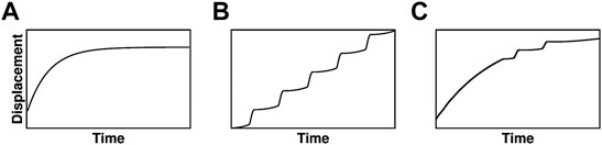
FIGURE 1. Schematic inflation regimes observed at volcanoes and mentioned within the text. (A) Inflation with a monotonically decaying rate often explained by the linear dynamics of pressure build-up within a storage zone through magma supply (e.g., Pinel et al., 2010). (B) Regime of successive transient inflation episodes superimposed onto an inflation with constant rate; this regime is referred to as “episodic inflation events” by Ji et al. (2017) and it is observed for example at Akutan volcano. (C) Episodic inflation events superimposed onto a longer period inflation with decaying rate (e.g., Walwer et al., 2019).

Other types of inflation patterns, such as successive transient inflation episodes superimposed onto longer-term inflation are also commonly observed; see Biggs and Pritchard (2017) and Figures 1B,C here. Such a pattern is sometimes referred to as “episodic inflation events” (Ji et al., 2017). At the Aleutian volcano Akutan, for instance, repeating transient inflation events are superimposed onto a secular linear inflation of the volcano (Walwer et al., 2016; Ji et al., 2017; Xue and Freymueller, 2020). Other volcanoes that exhibit repeating transient inflation events include Okmok (Alaska) and Piton de la Fournaise (La Réunion) (Peltier et al., 2008; Walwer et al., 2016; Xue and Freymueller, 2020).

The amplitude, spatial wavelength, and time scale of these events can vary significantly from one volcano to the other. As a result, these episodic inflation cycles are difficult to relate to a single physical process and are therefore sometimes interpreted as the result of ad hoc time-dependent forcing mechanisms, such as pulses of magma flux, degassing, or heat flux (Biggs et al., 2009; Peltier et al., 2009; Biggs et al., 2010; Xue and Freymueller, 2020). It is also worth noting that—in some cases, such as for the Okmok volcano and Piton de la Fournaise—successive inflation events do precede large eruptions while in other cases, such as at Akutan, they do not (e.g., Ji et al., 2017; Walwer et al., 2019).

Here we seek to extract temporal variability patterns from continuous deformation measurements at volcanoes that experience repetitive inflation events and to mine the available data for qualitative information on their underlying dynamics. To do so, we objectively extract repeating transient inflation signals at three volcanoes—Akutan, Okmok and Piton de la Fournaise—using a data-adaptive statistical methodology, namely Multichannel Singular Spectrum Analysis (M-SSA), applied to continuous GPS time series (Walwer et al., 2016).

These three volcanoes, which display such repetitive inflation events, have the advantage that their plumbing systems are well constrained by independent geochemical, petrological, seismic and geodetic datasets. We illustrate the resemblance of their deformation patterns using phase portrait reconstructions (Guckenheimer and Holmes, 1983; Ghil and Childress, 1987; Jordan and Smith, 2007), which indicate a striking dynamical similarity amongst them. To extract the dynamical features that lead to the observed phase portraits, we use a simple nonlinear oscillator that shares qualitative behavior with the inflation cycles observed at the volcanoes studied herein. This analogy, in turn, provides guidelines that we then use to build a physical model based on the plumbing system of the volcanoes being investigated.

The present paper aims in particular at presenting the connection between statistical analysis of GPS time series and dynamical modeling of volcanoes. The data used and the methods applied are presented in Section 2. In Section 3, we apply M-SSA to the GPS time series. The similarities in the phase portraits obtained for the three volcanoes are discussed in Section 4. The model for pressure build-up through magma flow between connected reservoirs is formulated in Section 5. Concluding remarks follow in Section 6 and we emphasize the consistency between our dynamical modeling approach and the amount of information contained in the geodetic data extracted and analyzed using our M-SSA methodology.

2 Data and Methods

2.1 Three Volcanoes and Their GPS Data Sets

We used position time series from continuous GPS data at stations located on three volcanoes: Akutan (8 stations) and Okmok (5 stations) in Alaska, and Piton de la Fournaise (10 stations) on La Réunion island (Figure 2). For Akutan the time series were taken from the Plate Boundary Observatory, pbo.unavco.org; they are expressed with respect to a North American Reference Frame. Time series recorded at Okmok and Piton de le Fournaise (PdF hereafter) were taken from the Nevada Geodetic Laboratory geodesy.unr.edu; they are expressed with respect to a North American reference frame and to the IGS international reference frame (IGS14), respectively (Blewitt et al., 2018). These time series contain the magmatic signals we are interested in, but also components of tectonic deformation, seasonal deformation due to atmospheric and hydrological processes, and GPS measurement noise.

FIGURE 2

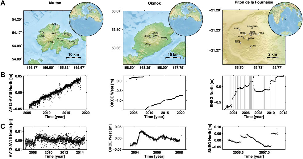
FIGURE 2. Location map and selected time series of GPS displacement for the three volcanoes used in this study. (A): Maps, with grey triangles showing the GPS sites from which the displacement time series used herein have been extracted; (B): Full time series available, including linear trend; (C): Selected time interval, with linear trend removed. The selected sites and directional components are indicated on the ordinate of the (B,C). For instance, for Akutan, AV12-AV15 North indicates the difference between the northward GPS displacements at sites AV12 and AV15. Grey vertical bars in the middle panels indicate intervals of eruptive activity.

Akutan and Okmok are located close to a subduction system where interseismic tectonic loading produces long-term deformation of the whole plate margin, including the volcanoes. At Akutan, the linear trend that dominates the variance of the time series is probably the result of this tectonic loading combined with a local volcanic inflation caused, for instance, by a constant magma flux into Akutan’s plumbing system. Following the approach of DeGrandpre et al. (2017), we remove the tectonic signal by considering the time series of baselines with respect to station AV15, the site farthest away from the volcanic center (Figure 2). This site is likely to record mainly tectonic deformation shared across the other Akutan GPS sites and it thus allows us to remove the common tectonic signal while conserving the magmatic signals we are interested in, including a linear volcanic inflation (DeGrandpre et al., 2017; Ji et al., 2017).

At Okmok, the smaller number of continuous GPS stations, together with gaps in the GPS time series at sites far away from the volcanic center, do not allow us to use the baseline approach described above for Akutan. However, volcanic signals at Okmok are of much larger amplitude, and InSAR time series, displayed in Biggs et al. (2010) for example, show that the GPS signals recorded before the 2008 eruption are superimposed onto a longer period signal with inverse exponential shape, characteristic of the dynamics of infilling of a magma reservoir (e.g., Reverso et al., 2014; Walwer et al., 2019). We therefore consider that the signals starting in 2003, before the 2008 eruption, mainly reflect volcanic deformation.

The PdF corresponds to an active hot spot within the Somalian tectonic plate; hence, no signal of tectonic loading is expected to be present in the deformation time series. Flank instability was associated with the 2007 co-eruptive and post-eruptive deformation events, but our study focuses on the signals preceding the 2007 eruption (Tridon et al., 2016; Poland et al., 2017).

2.2 Basic Ingredients of the M-SSA Analysis

In order to isolate the displacements associated with the activity of the volcanic systems from other geophysical signals—such as seasonal oscillations of atmospheric or hydrological origin—and from the GPS measurement noise, we filtered the position time series using M-SSA. M-SSA is a data-adaptive, non-parametric method that simultaneously exploits the spatial and temporal correlations associated with time evolving data sets (Ghil et al., 2002; Groth and Ghil, 2015; Alessio, 2016; Walwer et al., 2016). Apart from unraveling signals of different origins and signals from noise, M-SSA helps extract information about the underlying qualitative dynamics from the time series. The connection between M-SSA results of statistical time series analysis and dynamical systems behavior has been the subject of considerable research (Broomhead and King, 1986; Vautard and Ghil, 1989); it is exploited in Section 4.1 and Section 6.1 of the present paper.

M-SSA decomposes a set of D time series into modes of spatio-temporal variability that correspond to nonlinear trends, oscillations, or noise. These modes are derived from the eigenvectors of the covariance matrix:

$\mathbf{C}=\frac{1}{\left(N-M+1\right)}{\mathbf{X}}^{\text{t}}\mathbf{X}.(1)$

Here, C is computed from the ensemble of M lagged copies of the D time series composing the data sets and forming the columns of matrix X. This matrix, referred to as the “trajectory matrix,” provides a useful connection between M-SSA analysis and dynamical systems theory (Ghil et al., 2002) that is further exploited in Section 4.1.

The maximum period of the modes that can be extracted using the M-SSA is roughly Mτ_s, where τ_s is the sampling interval of the time series. Here we used τ_s = 1 day for the three GPS data sets analyzed for Akutan, Okmok, and PdF. The choice of M depends on the characteristics of the analyzed time series and the period of the signal one wants to extract.

The decomposition of the covariance matrix C given by

$\mathbf{\Lambda }={\mathbf{E}}^{\text{t}}\mathbf{C}\mathbf{E}(2)$

yields the D × M real eigenvalues that are the diagonal elements of Λ and the eigenvectors that appear as the columns of E. Signals that are strongly correlated in space and time in a given data set are captured as the modes with the largest eigenvalues. Here, we expect these modes to be signals of magmatic origin.

The projection of the time series and their lagged copies contained in the trajectory matrix X upon the eigenvectors gives the principal components (PCs) that form the columns of the matrix

$\mathbf{A}=\mathbf{X}\mathbf{E}.(3)$

The PCs are time series that represent the temporal behavior of the extracted modes. The variance of the data set described by each PC is given by the corresponding eigenvalue. The PCs can be seen as a sparse representation of the time-dependent patterns shared across a set of time series. They are a convenient tool for 1) visualizing the temporal shapes of the modes extracted by the M-SSA, and 2) identifying which modes may correspond to magmatic signals and which ones are more likely to represent either noise or geophysical signals of non-magmatic origin, such as seasonal oscillations caused by hydrological loads.

Once the modes corresponding to the magmatic deformation are identified, one can reconstruct the corresponding signal by projecting the PCs onto a set $\mathcal{K}\subset \left\{1,\dots ,DM\right\}$ of the eigenvectors:

$\mathbf{R}=\mathbf{A}\mathbf{K}{\mathbf{E}}^{\text{t}}={\mathbf{X}\mathbf{E}\mathbf{K}\mathbf{E}}^{\text{t}}.(4)$

This subset corresponds to the signal of interest, and K is a diagonal matrix of size DM × DM whose elements K_kk are 1 if $k\in \mathcal{K}$ and 0 otherwise. The reconstructed components, called RCs hereafter, provide the appropriate visualization of the signal after filtering out non-magmatic components and the lower-variance noise (Ghil et al., 2002; Alessio, 2016, and references therein). The RCs can also be used to represent the corresponding spatial deformation patterns at GPS in map view, for instance for selected time intervals (Walwer et al., 2016).

3 M-SSA Extraction of Episodic Inflation Events

3.1 Applying M-SSA to the GPS Data Sets

We performed the M-SSA analysis on GPS time series recorded at the three volcanoes under study, for time intervals that contain the same number of cycles for each volcano, i.e., three episodes of inflation Having the same number of episodic inflation events for the three volcanoes allows us to consistently compare and discuss the statistical information obtained, as well as the dynamics inferred therefrom.

Before applying M-SSA we removed the linear part of the time series that accounts for a large portion of the data variance. Removing the linear trend before applying M-SSA is commonly done to focus the analysis on the nonlinear part of the volcanic signal; see Walwer et al. (2016). Linear trends represent, in all likelihood, longer-term inflation upon which the nonlinear volcanic signal we are interested in is superimposed. While the time series analysis presented here focuses on the nonlinear signals, we do not preclude that the inflation trends play a role in the observed dynamics.

The connection between the extracted nonlinear signals and the long-term inflations is explained in Section 5.2 and discussed in Section 6.1 as well. Examples of detrended time series plotted over the selected time intervals are displayed in the Figure 2C. At Okmok and PdF, the last inflation episode—the few points ending the bottom time series in Figures 2 – precedes a large co-eruptive deflation event.

The main input parameter for the M-SSA analysis is the maximum lag Mτ_s used to compute the entries of the covariance matrix C in Eq. 1. Because the duration of the magmatic inflation events is different amongst the three volcanoes, the selected value of Mτ_s also differs for each data set. We use Mτ_s = 400 days for Akutan, Mτ_s = 150 days for Okmok, and Mτ_s = 30 days for PdF. The singular spectra—i.e., the normalized eigenvalues ranked in decreasing order—are displayed in Figure 3 together with the first 6 PCs. The relative variance captured by these PCs is given by the associated normalized eigenvalues, so that, for example, PC 1 at Akutan, Okmok and PdF describes respectively 5, 60 and 25% of the variance of the corresponding data set. Table 1 contains a summary of the characteristics of the data sets analyzed herein, together with the M-SSA input parameters and results.

FIGURE 3

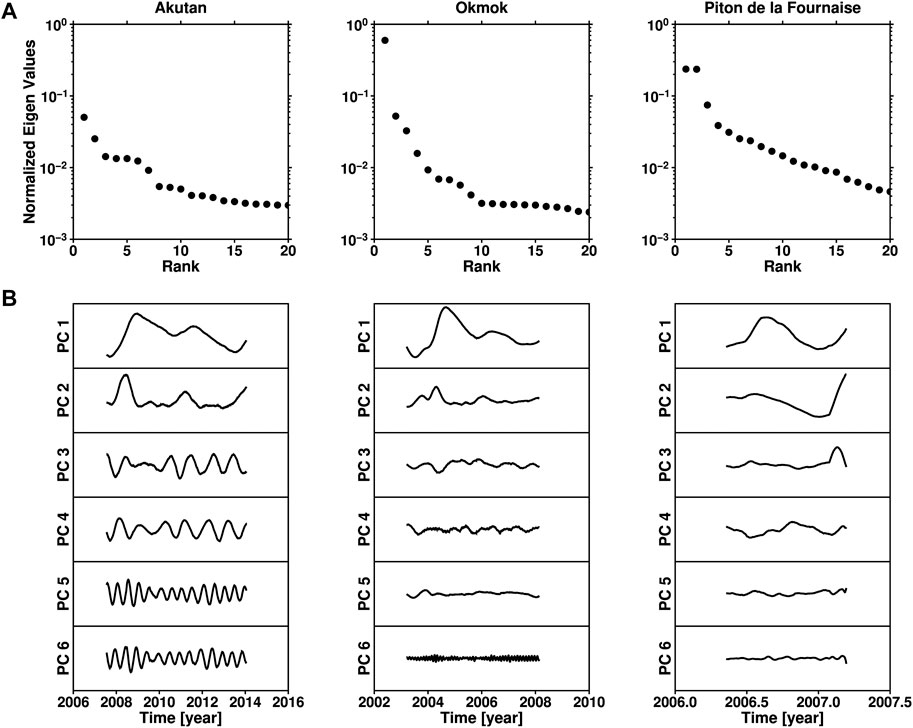
FIGURE 3. M-SSA analysis applied to the time series recorded at Akutan, Okmok and Piton de la Fournaise (PdF). The (A) show the normalized eigenvalues of the GPS position time series. (B) show the 6 leading PCs resulting from the M-SSA analysis applied to these three volcanoes.

TABLE 1

TABLE 1. Summary of the M-SSA parameters and of the results of the analysis, along with the characteristics of the deformation observed at the volcanoes investigated.

3.2 Mode Selection for the Volcanic Signals

We select the modes associated with magmatic signals based on their large variance and on two additional criteria. First, we search for temporal patterns that consist of relatively short inflations followed by longer intervals of rest or small-amplitude deformation. Because we detrended the time series before applying M-SSA, such a pattern corresponds to the PCs in Figure 3 that reflect intervals of increase in displacement, followed by a decrease in displacement. Second, we use the selected mode to reconstruct the corresponding nonlinear signals using Eq. 4, together with the extracted linear trend to represent the associated displacements in map view in order to check that the reconstructed spatial pattern is qualitatively consistent with volcanic inflation, i.e., radial displacements centered on the active crater that decay in amplitude with distance (Figure 4). The final check on the number of M-SSA modes S retained at each volcano relies on the consistency of the temporal and spatial pattern of the reconstructed displacements.

FIGURE 4

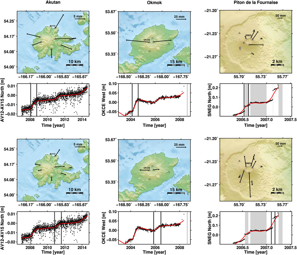
FIGURE 4. Spatial and temporal pattern of horizontal displacements at the three volcanoes. The two maps for each volcano show the total horizontal displacements (black arrows) during a selected episode of inflation; these episodes are indicated by the two vertical black lines on the time series corresponding to the map. The panels with the selected GPS time series display black dots for the raw GPS data points and a heavy red line for the sum of the corresponding M-SSA nonlinear volcanic signal reconstruction and linear trend. The GPS receivers associated with the plotted time series are labeled on the maps, as in Figure 2.

There is always a part of arbitrary decision when choosing the modes to reconstruct a given signal. The impact of this educated guesswork can be minimized by applying significance tests to specifically determine which modes are likely to be associated with colored noise, as opposed to a true geophysical signal. Varying the window size M within a reasonable range around the chosen values can constitute such a test. For the data sets at hand, we found that it does not affect the results of our analysis.

More sophisticated tests rely on the formulation of a null hypothesis against which the M-SSA results can be tested (Groth and Ghil, 2015). Such a test was performed for Akutan volcano by Walwer et al. (2016); we did not find it necessary to perform it for Okmok and PdF here, since the corresponding magmatic signals there are of much greater amplitude and readily visible in the data. Also, we observed that the reconstructed signal at the latter two volcanoes leads to spatial and temporal patterns that are quite consistent with the expectation of magmatic inflation–deflation events.

A key aspect of the M-SSA analysis, as further discussed in Section 6.1, is that the number of modes S used to reconstruct the signals is an output of the analysis itself. In the following, we provide details on how the leading modes were chosen in order to reconstruct the deformation signal for each volcano.

3.2.1 Akutan

Walwer et al. (2016) applied M-SSA to the Akutan GPS time series and the details provided there on the choice of the M-SSA parameters are not repeated here. The left panels of Figure 3 show the first 20 eigenvalues and the first 6 PCs obtained. One can clearly distinguish two groups of PCs: PCs 3–6 display oscillations with either an annual (PCs 3-4) or a semi-annual (PCs 5-6) period, while the combination of PCs 1-2 corresponds to a nonlinear trend that may include longer periods. PC 1 has an M-shape and captures the “skeleton” of the nonlinear trend associated with magmatic deformation, while PC 2 accounts for high-rate deformation that is correlated with the time intervals over which PC 1 displays an increase in displacement.

It follows that the best combination to use for reconstructing a spatially consistent volcanic signal is the combination of PCs 1 and 2. These two modes together account for roughly 7% of the detrended time series total variance. The corresponding spatial patterns for selected episodes of inflation, as well as an example of a M-SSA reconstructed time series that includes also the linear trend, are displayed in Figure 4. As expected, they show a clear radial displacement centered on the summit of the volcanic edifice, typical of a magmatic process.

3.2.2 Okmok

The singular spectrum at Okmok is displayed in the middle column of panels in Figure 3, along with the first six PCs. The first eigenvalue stands clearly above the rest of the spectrum and captures about 60% of the total variance. The associated PC has an M-shape very similar to PC 1 extracted at Akutan and, in the same way, captures the “skeleton” of the nonlinear temporal pattern of magmatic deformation.

The second PC, while accounting only for ∼6% of the detrended time series variance, captures a signal correlated with the first PCs and is needed to properly reconstruct the signal shown in Figure 4. We note here the striking similarities between the first two PCs at Akutan and Okmok, obtained without any a priori assumptions. These phenomenological similarities reflect, with some likelihood, a similarity between the dynamics underlying the two magmatic systems; see Section 4.1 below.

3.2.3 Piton de la Fournaise (PdF)

The singular spectrum for PdF in the right column of Figure 3 shows that the first two modes account for roughly 45% of the detrended time series total variance. As for PC 1 at Akutan and Okmok, these first two modes combined describe the “skeleton” of the nonlinear magmatic deformation pattern. The third eigenvalue stands also slightly above the rest of the modes, capturing about 10% of the total variance. The associated third PC has a peak that occurs simultaneously with the second episode of increase in displacement, as reflected by PCs 1 and 2. As for the PC 2 at Akutan and Okmok, PC 3 at PdF further emphasizes the asymmetry between the inflation episodes and the episodes of rest or small-amplitude deformation.

We selected, therefore, these first three modes to reconstruct the nonlinear volcanic signal at PdF (right panels in Figure 4). The reconstructed spatial patterns of displacement are more asymmetric than at Akutan or Okmok. This asymmetry is, most likely, a result of melt pressurization of shallow structures, such as dykes or sills, at PdF, instead of the deeper magma reservoirs present at the other two volcanoes (Peltier et al., 2008).

4 Similarities in Dynamical Behavior

4.1 Phase Portrait Reconstruction

To gain insight into the dynamics described by the filtered time series considered above, we now introduce a nonlinear relaxation oscillator whose solutions share certain key features with the behavior of all three volcanoes under study. The repetitive character of the transient inflation episodes studied herein motivates the use of an oscillator to provide phenomenological insights into mechanisms that may drive the cyclic behavior of interest.

Our highly idealized oscillator is not meant to explain the detailed physics of the natural processes at play. But it does help identify features that lead to the qualitative dynamical behavior observed in the data. These features, in turn, will serve as constraints for designing a physical model for the observed oscillations, as described in Section 5.2 below.

In order to identify the proper design features for our oscillator, we first compute phase portraits for the three volcanoes by plotting the PCs identified as magmatic signals in a phase plane (Packard et al., 1980; Roux et al., 1980; Takens, 1981; Gualandi et al., 2020). Such phase portraits show the evolution of a dynamical system as trajectories that contribute to a geometric representation of the system’s dynamics. In phase space, stationary solutions appear as fixed points and periodic ones as closed trajectories, called limit cycles (Guckenheimer and Holmes, 1983; Jordan and Smith, 2007). These representations highlight, in particular, how the dynamics of a system that is out of equilibrium is organized around equilibrium states (Ghil and Childress, 1987; Deremble et al., 2009). The goal here is to extract qualitative features of the magmatic systems’ dynamics.

The use of M-SSA to reconstruct phase portraits is inspired by the work of Broomhead and King (1986) and exploits several advantages of the M-SSA algorithm. First, the M-SSA results are obtained without a priori information on the dynamics that produced the volcanic signals. This is not necessarily the case for other signal processing techniques that use functions with predetermined temporal or spatial shapes to extract geophysical signals, and hence rely—sometimes implicitly—on assumptions about the underlying dynamics. Second, the connection between M-SSA and the qualitative dynamical study of physical systems is supported by theoretical, experimental, and observational work (Packard et al., 1980; Mañé, 1981; Takens, 1981; Broomhead and King, 1986; Vautard and Ghil, 1989). M-SSA can be seen as a particular formulation of the so-called “method of delays” that integrates observational time series into an embedding space through the construction of a trajectory matrix such as the matrix X introduced in Section 2.2. We refer the reader to Ghil et al. (2002) and (Alessio, 2016, Ch. 12) for comprehensive reviews of the connection between M-SSA and the dynamical study of natural systems from observational time series.

Reconstructed phase portraits for the three volcanoes are shown in Figure 5. The trajectories form almost closed orbits, typical of oscillatory behavior, with slight spiraling in and out. The striking similarities in the phase space structure of the trajectories drawn in Figure 5 between the three volcanoes indicate a dynamical similarity between them for the time intervals studied herein. A feature common to the phase portraits is that the trajectories are highly asymmetric about the horizontal line. This asymmetry is caused by PC 2 for Akutan and Okmok, and PC 3 for PdF. The latter PCs emphasize the relatively fast inflation episodes and further enhance the asymmetry between the deformation during the fast inflation events compared with the following, slower time intervals.

FIGURE 5

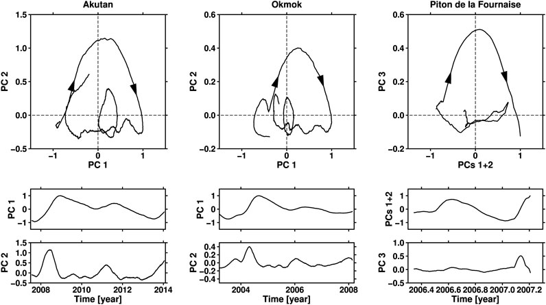
FIGURE 5. Phase portrait reconstructions that reflect the dynamics of the three volcanic systems under study. The (A) are the actual phase portraits, while the (B) below each phase portrait show the two PCs (for Akutan and Okmok) or three PCs (for PdF) used to reconstruct the trajectories in the phase plane.

Note that the phase portraits in Figure 5 that we reconstructed from the GPS time series correspond to a particular perspective on the phase space and the volcanoes’ dynamics. Alternative views of phase space trajectories can be constructed and may include, for example, the longer-period inflations that were initially removed but contain also information on the dynamics. The perspective we choose to display in Figure 5, however, contains the features we wish to focus on and serves well the line of reasoning presented in the following sections.

4.2 A Simple Conceptual Model

The phase portraits in Figure 5 indicate that further insight into the nature of the observed oscillations will be provided by formulating and analyzing a simple, nonlinear oscillatory model. The purpose of such a conceptual model is only to reproduce the first-order qualitative features of the phase portraits. As explained in the previous subsection, these phase portraits provide only one particular perspective upon the volcanic systems’ dynamics. Thus, the following conceptual model aims to replicate only the first-order features apparent from this perspective in order to gain basic insights into the dynamics associated with it. The choice of the model presented below is somewhat arbitrary and mainly motivated by its relative simplicity. Still, this exercise will help us formulate constraints relevant to the more detailed physical models described in Section 5.2.

Our conceptual model is governed by the following system of two coupled ordinary differential equations:

$\dot{x}=y,(\mathrm{5a})$

$\dot{y}=-\mu \left[x^2+{\left(y+y_0\right)}^2-1\right]y-x;(\mathrm{5b})$

here x and its time derivative y are the system’s two coupled variables, while μ and y₀ are independent parameters; see for example Jordan and Smith (2007). Both the dependent variables x, y and the independent variable t here are dimensionless.

The model governed by Eqs 5a, 5b contains the possibility of oscillatory solutions, as is the case for the following much simpler system that would be obtained, for instance, by setting μ = 0 in Eq. 5b

$\dot{x}=y,\dot{y}=-x.(6)$

Whether this ability to oscillate is realized for the system (Eqs 5a, 5b) depends on the model parameter values, as we shall see below. The simpler system (Eq. 6) is (a) linear, and (b) it is conservative, while system (Eqs 5a, 5b) is neither. The nonlinearity in Eqs 5a, 5b results from the form of the damping coefficient

$\kappa =\kappa \left(\mu ,y_0\right)\equiv -\mu \left[x^2+{\left(y+y_0\right)}^2-1\right].(7)$

The cases where κ < 0 and of κ > 0 are referred to as positive and negative damping, respectively.

For simplicity, let us assume that $y_0^2<1$. In this case, the regime into which the system evolves is controled by the value of μ. For μ < 0, κ < 0 in Eq. 7 as long as x² + y² is small enough and this regime has exactly one fixed point, i.e., one steady-state solution at the origin. This fixed point is linearly stable for the dissipative situation characterized by μ < 0. Linear stability means that, for any initial state sufficiently close to the origin, the system will spontaneously evolve towards the latter.

For μ = κ = 0, as in system (Eq. 6), there exist an infinite number of concentric, perfectly circular trajectories. When μ > 0, κ becomes positive, as long as x and y are located in the grey area of Figure 6, which contains the origin. This positive damping causes the origin to become unstable, and so the system’s trajectories spiral out, until they enter a region in which κ changes sign and thus limits further increase of the x² + y² distance from the origin. As a result, only a single closed trajectory exists, due to the damping. This trajectory is typically not circular, due to the nonlinearity, as illustrated by the one in Figure 6, computed for μ = 10.

FIGURE 6

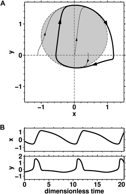
FIGURE 6. Nonlinear oscillation of the idealized model governed by Eqs 5a, 5b, for μ = 10 and y₀ = −0.6. (A): Phase portrait in the (x, y)-plane, with $y=\dot{x}$; (B,C): The associated time series representing, respectively, x(t) and y(t). In (A), the closed trajectory (heavy solid line) is the limit cycle. The light solid lines are typical trajectories converging to the limit cycle from the interior and the exterior of this cycle. The shaded area is the one where damping is negative, i.e., κ > 0 in Eq. 7. Arrows indicate the direction of motion on the limit cycle and on the trajectories that converge onto it.

The change in the dynamics of a nonlinear deterministic system from a unique stable fixed point to a stable closed orbit—such as the one seen in Figure 6—is called a Hopf bifurcation and the closed orbit itself is called a limit cycle (Guckenheimer and Holmes, 1983; Ghil and Childress, 1987; Jordan and Smith, 2007). The particular type of nonlinear oscillations that involve sawtooth-type behavior, as opposed to the sinusoidal oscillations of Eq. 6, with rapid escape from a no-longer stable fixed point followed by slow relaxation back to it, are called relaxation oscillations (Van der Pol, 1926; Ghil and Childress, 1987; Grasman, 2011; Ghil, 2019). In fact, the limit cycle in Figure 6 is precisely of the relaxation-oscillation type: not only is its shape not circular, but the velocities along it are nonuniform. This nonuniformity is highlighted by the changes in the slope of the x(t) and y(t) curves in the lower panels of Figure 6.

A first-order feature noticeable in Figure 6 that is common to the GPS observations at the three volcanoes studied here and is likewise present in the simple system governed by Eqs 5a, 5b is the alternation of intervals of fast increase in the observed quantities, followed by intervals with slower variations. For the three volcanoes, this correspond to relatively short and rapid inflation episodes, followed by longer intervals of small-amplitude deformation. This observed behavior is analogous to the fast increase in x(t), followed by its slower decrease, in the conceptual model.

We argue that, at the volcanoes being studied herein, these common patterns can be modeled as resulting from asymmetric oscillations similar to the ones in the conceptual model of Eqs 5a, 5b. This inference is also supported by the closed orbits of the phase portraits in Figures 5, 6. Pursuing this line of thought, one might suspect that the observed magmatic regime of the three volcanoes can be modeled as resulting from the loss of stability of an equilibrium point that is causing a Hopf bifurcation such as in the nonlinear oscillator of Eqs 5a, 5b.

Another important constraint we can extract from this analogy is that the “skeleton” of the dynamics—i.e., the main temporal pattern according to which these volcanic systems evolve—can be modeled by considering the interaction of merely two variables, like the two degree of freedom x and $\dot{x}=y$ of our conceptual model. This point is further discussed in Section 6.1 and supported by the statistical results obtained by M-SSA in Section 3.

Dynamical similarity does not necessarily imply physical similarity (Barenblatt, 2003). In the following section, however, we present a more complete physical model that shares some of the dynamical features described above, such as Hopf bifurcation, and provides new insights into the behavior of the three volcanoes studied herein.

5 Magma Flow Between Connected Storage Zones

We start this section by presenting evidence—for the three volcanoes studied herein—on a plumbing system composed of interconnected storage bodies fed by a deeper source. These storage bodies are either magma chambers or, as in the case of PdF, shallow networks of dykes and sills. The presence of interacting storage bodies is a key feature of the model presented in Section 5.2 below. This model aims to explain recurrent inflation events as reflecting an oscillatory regime caused by loss of stability of an equilibrium state in a manner that recalls the Hopf bifurcation in the conceptual model of Section 4.2.

5.1 Evidence for Connected Storage Zones of Magma

5.1.1 Akutan

The analysis of seismicity at Akutan volcano by Syracuse et al. (2015) highlights the elements that compose Akutan’s plumbing system. The precise location of seismic events shows that earthquakes beneath Akutan are clustered at depths that range between the near surface and roughly 30 km. Crustal seismic tomography shows a low-velocity zone located at depths of 7.5–10 km below the eastern flank of Akutan’s caldera (Syracuse et al., 2015). Interestingly, this low-velocity region seems to indicate the presence of storage zones that are distinct from the detected source of deformation located through geodetic data inversions around 4 km depth (Ji et al., 2017).

Moreover, part of the earthquakes occurring between 2003 and 2009 are low-frequency events (LFEs) at depths ranging from 10 to 27 km. LFEs are often interpreted as reflecting fluid transport in general, for instance episodes of magma transport (Power et al., 2004; Shapiro et al., 2018). They may indicate that a source supplies a part of the shallow plumbing system located around 7–10 km depth, which may in turn feed shallower storage zones. The latter could include, for example, the one detected by Ji et al. (2017) and located around 4 km depth (Syracuse et al., 2015).

Overall, seismic and geodetic observations at Akutan volcano point towards a plumbing system in which a deep reservoir supplies shallower melt bodies (Syracuse et al., 2015; DeGrandpre et al., 2017). This interpretation is also supported by the recent tomographic study of Koulakov et al. (2021), which provides a detailed imaging of Akutan’s plumbing system; see their Figure 8. Discrete inflation events, such as the ones displayed in Figure 4 herein, together with LFE occurrences, reflect discrete episodes of increase in the rate of shallow reservoir outflux (DeGrandpre et al., 2017).

5.1.2 Okmok

Different types of observations also indicate that Okmok’s plumbing system is composed of several melt storage zones, as briefly reviewed by Walwer et al. (2019). For instance, Larsen et al. (2013) found that the geochemistry and petrology of cones and vents created during the 1997 and 2008 eruptions implies melt sources coming from storage zones at distinct depths. In particular, more mafic material erupted during the 1997 eruption than in 2008, leading Larsen et al. (2013) to propose a deep storage body that feeds shallower reservoirs, inside which the magma evolution may vary from one eruption to the next.

Geodetic data sets also highlight the complexity of Okmok’s plumbing system. The spatial deformation pattern observed by GPS shows that both the 2008 source of precursory inflation—which occurred just before the eruption—and the source of the co-eruptive deflation are shallower and horizontally shifted from the source of the 1997 and 2008 deformation episodes (Freymueller and Kaufman, 2010). Xue et al. (2020) modeled the post-eruptive deformation in 2008 as resulting from the pressurization of a shallow sill fed by a deeper Mogi source. Moreover, InSAR time series from 1997 to 2008 recorded at Okmok reveal two successive episodes of inflation with a decreasing rate: one from 1997 to 2002 and then another one from 2002 to 2008; see Biggs et al. (2010), Figure 7 and Walwer et al. (2019), Figure 2. Walwer et al. (2019) interpreted this deformation sequence as reflecting interactions between two magma bodies.

FIGURE 7

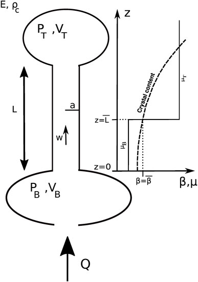
FIGURE 7. Schematic representation of the components of the physical model described in Section 5.2, including the key associated variables and parameters. Two reservoirs with volumes V_B and V_T, for bottom (B) and top (T), respectively, contain magma at pressures P_B and P_T. They are fed by magma from a deeper source region with constant flux Q. The pipe linking the two reservoirs has radius a and length L, and the magma flows through it at velocity w. Inside the pipe, the crystal concentration β per volume reaches the value $\bar{\beta }$ when $z=\bar{L}$. Above $\bar{L}$ the viscosity increases from μ_B to μ_T.

A schematic plumbing system for Okmok, inferred from a combination of geodetic, geochemical, and petrological data, is depicted in Larsen et al. (2013), their Figure 14). It indicates that several shallow melt bodies are connected to a deeper, mid-crustal magma reservoir that is itself supplied with basaltic magma from greater depths.

5.1.3 Piton de la Fournaise (PdF)

Peltier et al. (2009) reviewed geochemical and petrological data from PdF and showed that several types of lavas erupted during its recent activity. Minerals in some lava bodies crystallized in a shallow storage zone located at roughly 2 km depth (Famin et al., 2009). Melt inclusions in materials from the 2005 eruptions show that the crystallization of olivine occurred at shallow depths of 0–2.5 km (Famin et al., 2009). The maximum estimated depth for the entrapment of melt inclusions is consistent with the estimated depth of the source of deformation determined from geodetic measurements, as well as with the source of most earthquakes located between 200 m and 2.5 km below the surface (Peltier et al., 2009). According to Peltier et al. (2008), the corresponding reservoir is likely to be connected to a shallow network of dykes and sills that regularly get pressurized and produce episodic inflation events, such as the ones displayed in Figure 4 herein.

The geochemistry of the lava from the 1998 eruption shows that it underwent fractionation, which indicates a deeper origin and is consistent with seismic events in 2005 and 2008 located at depths of around 7.5 km (Battaglia et al., 2005; Boivin and Bachèlery, 2009). Battaglia et al. (2005) describe a seismic swarm migrating from 7.5 km to the surface before the March 1998 eruption.

All together, the observations summarized above show that the PdF plumbing system contains at least two reservoirs. One corresponds to the source of surface inter-eruptive deformation and is located at a depth of about 2 km. It supplies an overlying network of dikes and sills generating the episodic inflation events such as the ones displayed in Figure 4, together with eruptive activity. A second reservoir corresponds to a source of deeper seismicity at about 7.5 km depth. A schematic representation of the PdF plumbing system is proposed in Famin et al. (2009), Figure 8.

FIGURE 8

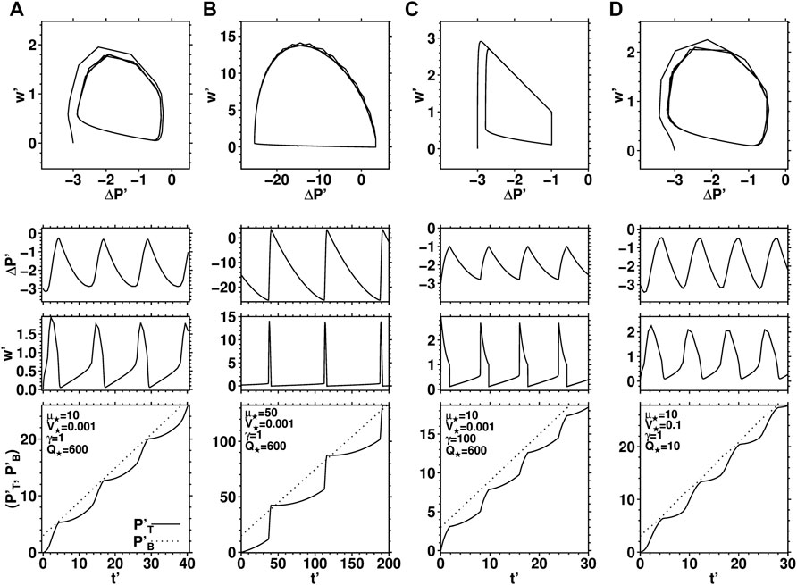
FIGURE 8. Nonlinear pressure oscillation of the idealized physical model governed by Eqs 9a, 9b. Top panels represent the phase portraits of the simulation in the (ΔP′, w′) plane. Subsequent panels represent, from top to bottom: Time series of ΔP′(t′); time series of w′(t′); and time series of $P_B^{\prime }(t^{\prime })$ (dotted) and $P_T^{\prime }(t^{\prime })$ (solid). The model solutions were computed using the following sets of parameters: (A) (μ_⋆, V_⋆, γ, Q_⋆) = (10, 0.001, 1, 600); (B) (μ, V_⋆, γ, Q_⋆) = (50, 0.001, 1, 600); (C) (μ_⋆, V_⋆, γ, Q_⋆) = (10, 0.001, 100, 600); (D) (μ_⋆, V_⋆, γ, Q_⋆) = (10, 0.1, 1, 10). All variables and parameters are expressed in dimensionless form.

5.2 A Model of Interacting Storage Zones

5.2.1 Basic Geophysical Insights

In Section 4.1, we showed that a nonlinear oscillator captures key features of the qualitative dynamics of the three volcanoes studied herein. We then described evidence for connected magma storage bodies—whether magma reservoirs or a reservoir connected to a shallow network of dykes and sills—for all three volcanoes. We now present a more detailed physical model that builds upon these findings and produces relaxations oscillations similar to the observed ones.

Before formally describing the model, let us first provide some basic insights into the mechanisms at play. Our model treats magma transport as driven by pressure variations between two storage bodies, a shallower and a deeper one. This scheme is typical of models often used for magma plumbing systems (Lenglin et al., 2008; Pinel et al., 2010; Reverso et al., 2014). Here, however—depending on the characteristics of the plumbing system being modeled, as described in Section 5.1—these two bodies correspond either to lower and upper crustal magma bodies or to two relatively shallow magma bodies, the latter being more appropriate for the PdF plumbing.

In our case, the deeper storage is fed from below at a constant rate, so that the transient inflation events described above are not a result of ad hoc variations in the overall magma flux, contrary to most other approaches. As magma flows from the deeper storage body into the shallower one, it undergoes decompression-induced crystallization that leads to a viscosity increase in the connecting conduit. The resulting larger viscosity lowers the efficiency of the hydraulic connection between the two storage bodies, which eventually cancels out the pressure gradient driving the flow.

As the deeper storage zone keeps being supplied from below at a constant rate, its pressure continues to build up. Under such circumstances, the viscosity-dependent velocity of the magma flow connecting the two storage zones can exhibit a sudden pulse to reduce the pressure gradient and bring the system closer to its equilibrium state of equal pressure between the two storage zones.

When the proper conditions are met, this phenomenon repeats, so that pressure in the top storage zone builds up in a staircase manner, i.e., with transient episodic increases in pressure. This pressure build-up regime is of the relaxation oscillation type, and thus dynamically similar to the one presented in Section 4.2, which also explains the occurrence of sharp pressure variations between the storage zones that alternate with more gradual variations. We argue that these transient increases in pressure in the uppermost storage zone are the cause of the episodic inflation events described in Section 3.2.

5.2.2 Mathematical Model Formulation

A schematic representation of our model is displayed in Figure 7 and the associated variables and parameters are summarized in Table 1. Formally, a hydraulic connection of length L and radius a links two storage bodies of volumes V_T and V_B, with pressures P_T and P_B. Subscripts B and T refer to bottom and top, respectively. The bottom body is fed with from below with constant magma flux Q.

The magma rises through the conduit between the two storage bodies with an horizontally averaged vertical velocity w. Doing so, the magma viscosity changes. Several mechanisms can lead to this; here we assume that viscosity increases as a result of decompression-induced crystallization, as described by Blundy and Cashman (2001) for instance. This mechanism is motivated by the observations at Okmok and PdF, where Larsen et al. (2013) and Famin et al. (2009) have described evidence of crystallization and degassing during magma ascent. We follow Barmin et al. (2002) and consider that, along the conduit, the viscosity is given by a step function and switches from the constant value μ_B to the constant value μ_T when the crystal content β per volume reaches the threshold value $\bar{\beta }$ (Figure 7).

The model presented here builds upon the insights of Whitehead and Helfrich (1991) and Barmin et al. (2002) on velocity-dependent viscosity in magmas; further details on its derivation are provided by Walwer et al. (2019) and in Supplementary Appendix SB of the present paper as well. The resulting system of equations

$\begin{array}{cc}\hfill & \frac{\text{d}{P}_B}{\text{d}t}=Q-w\frac{E\pi a^2}{V_B},\hfill \\ \hfill & \frac{\text{d}{P}_T}{\text{d}t}=w\frac{E\pi a^2}{V_T},\hfill \\ \hfill & \frac{\text{d}w}{\text{d}t}=\left\{\begin{array}{cc}\hfill & -\frac{1}{L\rho }\left(\left(P_T-P_B\right)+\rho gL\right)-\frac{8w\left({\mu }_B-{\mu }_T\right)\bar{L}}{a^{2}L}-\frac{8w{\mu }_B}{a^2}\mathrm{f}\mathrm{o}\mathrm{r}w\le \bar{w},\mathrm{a}\mathrm{n}\mathrm{d}\hfill \\ \hfill & -\frac{1}{L\rho }\left(\left(P_T-P_B\right)+\rho gL\right)-\frac{8w{\mu }_B}{a^2}\mathrm{f}\mathrm{o}\mathrm{r}w>\bar{w}\hfill \end{array}\right.\hfill \end{array}(8)$

governs the joint temporal evolution of the bottom and top pressures, P_B and P_T, as well as of the vertical velocity w. It is derived from the coupling between the horizontally averaged vertical magma momentum equation, elastic deformation induced by volume changes in the magma bodies that have a bulk modulus equals to E, and the chemical kinetics of magma crystallization that relates the rate of decompression, proportional to w, to the viscosity through crystal content β. System (Eq. 8) reduces to the linear dynamics of reservoir pressure variations commonly used to model observed volcanic inflation or co-eruptive subsidence with decaying exponential shape when no change in viscosity occurs in the conduit (e.g., Dvorak and Okamura, 1987; Reverso et al., 2014).

The derivation of system (Eq. 8) follows the Whitehead and Helfrich (1991) approach and relies on the introduction of the length scale $\bar{L}$ that corresponds to the height above which enough crystallization occurs in order for the viscosity to transition from μ_B to μ_T (Figure 7). A key point is that $\bar{L}$ depends on the decompression rate and therefore on the vertical magma velocity w, thus conferring a nonlinear character to system Eq. 8. The velocity scale $\bar{w}$ is obtained by posing $L=\bar{L}$ in such a way that, if $w>\bar{w}$, the decompression rate is too high for significant crystallization to occur and the magma exhibits no change in viscosity; hence the two forms taken by dw/dt in (Eq. 8) depend upon the value of w.

The study of system (Eq. 8) can be simplified by expressing it in a nondimensional form and by considering the pressure difference ΔP = P_T − P_B rather than P_T and P_B individually. The model leads to the following dimensionless set of ordinary differential equations, in which all dimensionless variables are denoted by a prime and govern the time evolution of the dimensionless pressure difference $\mathrm{\Delta }{P}^{\prime }=P_T^{\prime }-P_B^{\prime }$ and of the vertical magma velocity w′:

$\frac{\mathrm{d}\mathrm{\Delta }{P}^{\prime }}{\mathrm{d}{t}^{\prime }}=-V_{\star }{Q}_{\star }+\left(1+V_{\star }\right)w^{\prime },(\mathrm{9a})$

$\frac{\mathrm{d}{w}^{\prime }}{\mathrm{d}{t}^{\prime }}=\gamma \left(g\left(w^{\prime }\right)w^{\prime }-\mathrm{\Delta }{P}^{\prime }\right),(\mathrm{9b})$

where

$g\left(w^{\prime }\right)=\left\{\begin{array}{cc}\hfill & \left({\mu }_{\star }-1\right)w^{\prime }-{\mu }_{\star }\mathrm{f}\mathrm{o}\mathrm{r}{w}^{\prime }\le 1,\mathrm{a}\mathrm{n}\mathrm{d}\hfill \\ \hfill & -1\mathrm{f}\mathrm{o}\mathrm{r}{w}^{\prime }>1.\hfill \end{array}\right.(10)$

The scales used to transform the system (Eqs 9a, 9b) to the nondimensional version are:

$w=\bar{w}{w}^{\prime },\bar{w}=\frac{{\left(36\pi n_{ch}\right)}^{1/3}{\bar{\beta }}^{2/3}\chi L}{\mathrm{\Delta }\beta },(\mathrm{11a})$

$t=\bar{t}{t}^{\prime },\bar{t}=\frac{8\rho {\mu }_{B}L{V}_{\text{T}}}{E\pi a^4},(\mathrm{11b})$

$\mathrm{\Delta }P=\bar{p}\mathrm{\Delta }{P}^{\prime }=\bar{p}\left(P_T^{\prime }-P_B^{\prime }\right),\bar{p}=\frac{L\rho 8{\mu }_{\text{T}}\bar{w}}{a^2},(\mathrm{11c})$

$Q=\bar{Q}{Q}_{\star },\bar{Q}=\pi \bar{w}{a}^2.(\mathrm{11d})$

The velocity scale $\bar{w}$ is the threshold below which crystal content increases significantly, hence resulting in a viscosity change; see Barmin et al. (2002), Walwer et al. (2019) and Supplementary Appendix SB herein. The time scale $\bar{t}$ is the characteristic time derived from a linear hydraulic model of pressure balance between two reservoirs (Pinel et al., 2010), while $\bar{p}$ is the viscous pressure scale that arises from the steady-state, horizontally averaged vertical momentum conservation (Jaupart and Tait, 1990; Whitehead and Helfrich, 1991).

5.2.3 Conditions for Pressure Oscillations

The four dimensionless parameters that control the dynamic behavior of the system are:

${\mu }_{\star }=\frac{{\mu }_{\text{T}}}{{\mu }_{\text{B}}},V_{\star }=\frac{V_{\text{T}}}{V_{\text{B}}},\gamma ={\left(8{\mu }_{\text{B}}\right)}^2\frac{\rho L{V}_{\text{B}}}{E\pi a^6},Q_{\star }=\frac{Q}{\bar{w}\pi a^2},(12)$

where ρ is the magma density, E an elasticity coefficient linking the volume variation with the pressure variation inside the magma reservoirs, and μ_B and μ_T the viscosity in the lower and the upper parts of the conduit, respectively (Whitehead and Helfrich, 1991; Walwer et al., 2019).

Note the similar relationship between variables x and y in the conceptual model (Eqs 5a, 5b), with $\dot{x}\propto y$ and $\dot{y}\propto -x$, and the variables ΔP′ and w′ in the physical model governed by Eqs 9a, 9b, with $(\dot{\mathrm{\Delta }{P}^{\prime }})\propto w^{\prime }$ and ${\dot{w}}^{\prime }\propto -\mathrm{\Delta }{P}^{\prime }$. Moreover, the nonlinear function g (w′) in Eq. 9b plays a role analogous to the nonlinear damping κ(y) in (Eq. 5b). As a result, the physical model (Eqs 9a, 9b) also contains the possibility of oscillatory solutions arising from the stability loss of the equilibrium state. This situation is met when:

${\mu }_{\star }>2(13)$

and when the magma flux Q_⋆ satisfies the following two-sided inequality

$\frac{V_{\star }+1}{V_{\star }}>Q_{\star }>\frac{1}{2}\frac{\left(V_{\star }+1\right){\mu }_{\star }}{V_{\star }\left({\mu }_{\star }-1\right)}(14)$

These two inequalities imply that the pressure oscillations can only arise when 1) the magma undergoes a large enough change in viscosity as it flows from the bottom magma body to the top one; and 2) the magma flux feeding the system is also bounded in magnitude according to Eq. 14. The inequalities Eq. 14 constitute one of the key insights provided by our modeling approach and show how the history and the rate at which the magma enters the plumbing system can affect its dynamics. If the magma flux is too low or too high no sustained oscillations of magma pressure within the storage zones are possible. This result is further discussed in the Section 6.2 in relation to observations at Akutan, Okmok and PdF.

Phase portraits of the physical model in the relaxation oscillation regime are displayed in Figure 8 for the four sets of the dimensionless parameters defined in Eq. 12; each set of parameters corresponds to the panels in one of the figure’s columns (a)–(d). The trajectories asymptote in each case to closed orbits, as for the phase portraits derived from the data in Figure 5 and those of the conceptual model in Figure 6.

The sawtooth-shaped oscillations of ΔP′(t′) in Figure 8 resemble the oscillations of x(t) in Figure 6. The ΔP′(t′) oscillations reflect pulses of magma flow velocity increase w′(t′) in the connecting pipe that are analogous to the $\dot{x}=y(t)$ pulses in Figure 6. While $P_B^{\prime }(t^{\prime })$ increases linearly (dotted lines in the bottom row of panels in Figure 8), due to the constant flux Q_⋆, these w′(t′) pulses cause sharp periodic pressure variations of ΔP′(t′) (middle row of panels in Figure 8). As a result, $P_T^{\prime }(t^{\prime })=P_B^{\prime }(t^{\prime })+\mathrm{\Delta }{P}^{\prime }(t^{\prime })$ in the top storage zone (solid line in the bottom panels) exhibits the staircase-shaped pattern in the bottom panels of Figure 8.

The latter temporal patterns are a simplified, purely periodic version of the more irregular patterns observed at the three volcanoes in Figure 4. Both the model and the observations show episodes of fast and short pressure increases, followed by episodes of longer and slower pressure decreases. We also note, in the top row of panels of Figure 8, that the amplitude of the oscillations only depends on the system’s parameter values and not on the initial state from which they arise. This independence of initial state seems to also characterize the observations in Figure 4, as far as the limited data sets allow such inferences to be made.

Finally, the degree of asymmetry, the period, and the amplitude of the pressure oscillations in the physical model are also controlled by the dimensionless parameters μ_⋆, γ, V_⋆ and $\left.Q_{\star }\right)$. Panels in columns (a)–(d) of Figure 8 show model results for a range of parameter values. We observe that the larger the viscosity ratio μ_⋆, the longer the period of the oscillation and the larger their amplitude; see Figures 8B vs. Figure 8A.

Parameter γ mainly controls the asymmetry of the oscillations, with larger values of γ creating sharper variations of pressure; see Figures 8C vs. Figure 8A. Note that when the ratio V_⋆ = V_T/V_B varies, the flux Q_⋆ has to be adjusted to satisfy the two-sided inequality (Eq. 14), so that the system generates pulses of pressure increase; see Figures 8D vs. Figure 8A. The quantitative implications of the physical model in this section, in particular inequalities (Eq. 14), are discussed in Section 6.2 and Section 6.3.

6 Discussion

6.1 M-SSA, Parsimonious Modeling, and the Dynamics of Volcanic Systems

In Section 2, we used multichannel singular spectrum analysis (M-SSA) of GPS time series to characterize the qualitative dynamics of three volcanic systems: Akutan, Okmok and Piton de la Fournaise (PdF); see Figures 2–5. We then showed in Section 4 that a highly idealized conceptual model governed by Eqs 5a, 5b can explain the common qualitative dynamics of these three volcanic systems; see Figure 6.

The basic features of the conceptual model and the similarities between the phase portraits in Figures 5, 6 helped us formulate in Section 5 a still fairly simple physical model of a magmatic system with two storage bodies connected by a conduit in which magma flows with a time-dependent viscosity. Both the conceptual model of Section 4.2 and the physical model of Section 5.2 possess only 2 variables, often referred to in the physical sciences as two degrees of freedom.

An important aspect of our statistical time series analysis is that the number of leading modes S retained to construct the volcanic deformation signal displayed in Figure 4 and the phase portrait in Figure 5 is quite small, namely 2 ≤ S ≤ 3. From the perspective of extracting information about the dynamics of natural systems using M-SSA, the number of modes S retained to reconstruct the signals of interest has been referred to as the statistical dimension of the system (Vautard and Ghil, 1989).

This S corresponds to an upper bound on the number of degrees of freedom required for a parsimonious description of the underlying dynamics within the accuracy of the data. It accounts for the amount of information contained in the observations, which is limited by the noise and the discrete sampling (Broomhead and King, 1986; Vautard and Ghil, 1989). Another important limitation of the information available on volcanic systems is the fact that geophysical observations are often indirect measurements of the systems under study and constitute therewith only indirect constraints on the quantities we are interested in. In the present case, geodetic data sets provide indirect information about pressure evolution inside volcanic plumbing systems.

Vautard and Ghil (1989) showed that the value of S used to reconstruct an observed signal is not unique and depends on the data quality as well as on the key M-SSA parameters: the number of data points N in each time series, the number D of time series or “channels,” and the window length M. These authors showed that increasing M or the signal-to-noise ratio tends to increase S. Because of the characteristics of the data sets used here, M and the signal-to-noise ratio are indeed different for each volcano, as described in Table 1. Still, a common feature of the three M-SSA analyses is that the volcanic signal reconstructions result in using a very small number of modes S.

Together, the small number S of leading modes needed to describe the deformation signal, and the two degrees of freedom of the conceptual model that capture the key features of the data sets, suggest that the number of variables needed to describe the dynamical state of the volcanic systems studied here during the time interval under consideration and within the accuracy of the data is also quite small (Farmer et al., 1983; Broomhead and King, 1986; Vautard and Ghil, 1989). Two interpretations can be proposed to explain this striking result. First, the observations themselves, i.e., the time-dependent deformation data, only provide limited information on the mechanism leading to the observed signal. Second, although volcanic systems a priori possess a large number of degrees of freedom, the qualitative nature of the oscillatory phenomenon observed herein reflects a form of self-organization that requires only the interaction of a few variables to generate the “skeleton” of the observed dynamics (Guckenheimer and Holmes, 1983; Carr, 2012). In any case, reduced dynamical systems, be they simple conceptual models or more detailed physical models of an idealized plumbing system, provide useful frameworks to model the observations presented here.

The temporal pattern of deformation observed herein at three volcanoes can thus be explained by a parsimonious nonlinear model of magma body interaction with velocity-dependent magma viscosity in the rising magma. The connection between a data-adaptive time series analysis method and a parsimonious physical model provides an interesting guideline for understanding and modeling volcanic episodic inflation events. Whether or not the specific proposed mechanism, i.e., viscosity variation through decompression-induced crystallization, is the most appropriate one remains to be established. But it seems fairly clear that physical models capable of explaining deformation observations should possess a Hopf bifurcation from a fixed point to a limit cycle that gives rise to asymmetric, sawtooth-shaped oscillations.

It is worth mentioning here that models involving other physical mechanisms with qualitatively different viscosity profiles can display similar behavior (e.g., Whitehead and Helfrich, 1991; Walwer et al., 2019). Altogether, these models show that the key ingredient from which of relaxation oscillations of magma pressure arise is the nonlinear coupling between the flow velocity and the flow resistance. This is somewhat analogous to the phenomenon of velocity-weakening of friction that can lead, in similar ways, to the oscillatory behavior of systems with frictional interfaces (e.g., Gu and Wong, 1994; Marone, 1998).

The present work could thus stimulate new research to determine to which extent volcanic inflation cycles may lie—for a given set of parameter values—in a stable oscillatory regime or, to the contrary, be subject to an instability that, in turn, may lead to eruptive behavior, as observed at PdF and Okmok in 2007 and 2008, respectively (Larsen et al., 2013; Rivet et al., 2014). Being able to distinguish between these two regimes also hints at the possibility of understanding the eruptive potential of such volcanoes by monitoring possible transitions from the oscillatory to the runaway regime.

6.2 Long-Term Inflation Trend and the Flux of Magma Entering the Plumbing System

The long-term inflation trend reflects the temporal pattern of magma supply from depth into the plumbing system modeled here. The model of Figure 7 implies that the pressure oscillations giving rise to the episodic inflation events are sustained only when the volumetric flux of magma Q feeding the system is bounded by the values expressed in inequality (Eq. 14). At Akutan, the linear long-term trend suggests that Q is constant, which may explain why the episodic inflation events are sustained over time and repeat regularly. The same is true for PdF, where inflation events occur frequently from 2004 to 2007; see again Figure 2.

A key difference between Akutan and PdF, however, is that the amplitude and time interval between successive events are relatively similar for the former, while for the latter they exhibit more variations, as well as small eruptive events (Figure 2). The dynamical regime observed in the GPS time series may be qualified as more chaotic for Pdf in opposition to the seemingly regular occurrences of transient inflation events observed at Akutan.

At Okmok, the episodic inflation events preceding the 2008 eruption occurred at the end of an inflation episode with a decaying rate that started in 2002 (Biggs et al., 2010; Walwer et al., 2019). We infer that the magma flux was too large at the beginning of this inflation episode to produce sustained pressure oscillations and only dropped into the proper range, given by (Eq. 14), afterwards (Walwer et al., 2019).

Quantitative estimates of the volumetric flux of magma supply into the plumbing system for all three volcanoes are on the order of Q ∼ 10⁶ m³/year (Peltier et al., 2008; Fournier et al., 2009; Xue and Freymueller, 2020). At Okmok, this value corresponds to the estimated volumetric flux before the occurrence of the inflation events studied here (Fournier et al., 2009, Figure 12). A corresponding value for the dimensionless flux that intervenes in the model governed by Eqs 9a, 9b is Q_⋆ ≃ 500 (Table 2). From inequality Eq. 14, this implies that the volume ratio V_⋆ is on the order of 10⁻³ for the three volcanoes. At Akutan, estimated values for the volume of the storage bodies are in the range 10⁻⁵ − 1 km³ (DeGrandpre et al., 2017, Tables 4 and 6). At PdF, the shallow structure causes the deformation to arise from a network of dykes and sills that most likely have significantly smaller volume than the deeper reservoir connected to it. Hence, V_⋆ ≃ 0.001, i.e., the bottom storage zone V_B, quite plausibly, has a volume that is roughly 1,000 times larger than the uppermost body’s volume V_T.

TABLE 2

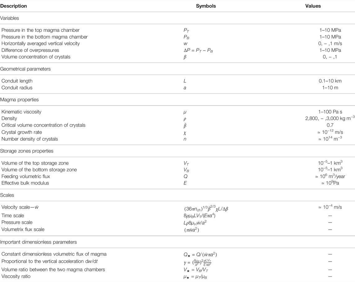
TABLE 2. List of main variables and parameters described in the main text and appearing in the proposed physical model of Section 5.2.

6.3 Temporal and Spatial Patterns of the Volcanic Deformation

A substantial difference between the volcanoes studied here consists in their characteristic time scales and deformation wavelengths (Table 1). Akutan and Okmok deformed over a distance of roughly 10 km with a delay between two inflation events of around 2 and 3 years, respectively. The events at PdF have noticeably smaller spatial wavelengths, of about 2 km, and the delay between successive events is of a few days (Table 1). The spatial deformation pattern at PdF also shows azimuthal asymmetries during inflation events (Figure 4), probably caused by the pressurization of small shallow structures such as dykes and sills, as described above, that are connected to the surface and produce co-occurring eruptive activity (Peltier et al., 2008; Famin et al., 2009).

Deformation cycles of shorter duration thus correlate with smaller deformation wavelength, an observation consistent with model (Eqs 9a, 9b) presented in Section 5.2. The spatial deformation wavelength is a function of both size and depth of the structures producing the observed GPS displacements. The time scale used to render Eqs 9a, 9b dimensionless is proportional to the volume V_T of the shallow storage body (Table 2). All else being equal, the smaller the volume V_T, the smaller the time scale and the shorter the duration of the episodic inflation events. Overall, the simple and parsimonious model governed by Eqs 9a, 9b can account for the spectrum of observed time scales and deformation scales at Akutan, Okmok, and PdF.

7 Conclusion

Our paper strongly suggests that mechanisms resulting from 1) the presence of two or more magma bodies and 2) the mere dependence of the magma’s flow resistance on temperature or crystallisation in the conduit between these bodies can explain key features of the observed recurrent inflation episodes in rather diverse volcanoes. The presence of these two key ingredients in many active volcanic systems suggests that our model may apply fairly broadly, beyond the three examples used here.

A more complete explanation of the currently available information in the geodetic and geochemical evidence will require, of course, more detailed modeling and, possibly, additional observations. At this stage, though, it does not appear that external forcing by time-dependent magma inflow is essential for the explanation of the most salient aspects of the alternation of rapid inflation with longer episodes of relatively low level of deformation.

The phenomenological approach presented herein starts with the statistical analysis of geodetic time series and ends with the construction of a relatively simple physical model of volcanic plumbing systems. The connection between the observational data and the physical model is provided by the study of a simple nonlinear oscillator’s capturing key features of the observations.

This approach can be applied to help understand a wide range of observed temporal patterns of deformation. It is, therefore, not restricted to the type of behavior studied herein. The two relatively simple models presented, conceptual (Section 4.2) and physical (Section 5.2), can be seen as a contribution to a hierarchy of models with increasing complexity—from the very simplest conceptual models to high-resolution, three-dimensional ones—that share important features and thus can provide more and more details on the phenomena under study. A model hierarchy of this kind is fairly common in other areas of the geosciences, such as the climate sciences (Schneider and Dickinson, 1974; Ghil et al., 2001; Held, 2005; Ghil, 2019).

Data Availability Statement

Publicly available datasets were analyzed in this study. This data can be found here: www.earthscope.org geodesy.unr.edu.

Author Contributions

DW, MG, and EC designed the study. DW conducted the data analysis and the model studies. All authors discussed the results and implications and commented on the manuscript at all stages.

Funding

This research was supported by a doctoral grant from PSL Research University (DW), and by research Grant No. 9AD01274 from the INSU/CNRS program Programme National de Télédétection Spatiale (PNTS) (EC). The present paper is TiPES contribution #128; this project has received funding from the European Union’s Horizon 2020 research and innovation programme under Grant Agreement No. 820970.

Conflict of Interest

The authors declare that the research was conducted in the absence of any commercial or financial relationships that could be construed as a potential conflict of interest.

Publisher’s Note

All claims expressed in this article are solely those of the authors and do not necessarily represent those of their affiliated organizations, or those of the publisher, the editors and the reviewers. Any product that may be evaluated in this article, or claim that may be made by its manufacturer, is not guaranteed or endorsed by the publisher.

Acknowledgments

We are grateful to Claude Jaupart for insightful discussions. It is a pleasure to thank Andreas Groth for sharing his M-SSA codes and for helping us with certain aspects of practically implementing the M-SSA methodology. DW thanks Pascal Richet for his thoughtful comments and corrections on the first version of the manuscript. It is a pleasure to acknowledge two reviewers as well as Valerio Acocella for constructive and insightful comments and suggestions on the paper’s originally submitted manuscript. EC acknowledges support from the Institut Universitaire de France. This work uses data products provided by the Plate Boundary Observatory operated by UNAVCO for EarthScope (www.earthscope.org) and by the Nevada Geodetic Laboratory (geodesy.unr.edu).

Supplementary Material

The Supplementary Material for this article can be found online at: https://www.frontiersin.org/articles/10.3389/feart.2022.759475/full#supplementary-material

References

Alessio, S. M. (2016). “Singular Spectrum Analysis (SSA),” in Singular Spectrum Analysiss (SSA) (Berlin, Germany: Springer), 537–571. Ch. 12. doi:10.1007/978-3-319-25468-5_12

CrossRef Full Text | Google Scholar

Barenblatt, G. I. (2003). Scaling, Vol. 34. Cambridge: Cambridge University Press.

Google Scholar

Barmin, A., Melnik, O., and Sparks, R. S. J. (2002). Periodic Behavior in Lava Dome Eruptions. Earth Planet. Sci. Lett. 199, 173–184. doi:10.1016/s0012-821x(02)00557-5

CrossRef Full Text | Google Scholar

Battaglia, J., Ferrazzini, V., Staudacher, T., Aki, K., and Cheminée, J.-L. (2005). Pre-eruptive migration of earthquakes at the Piton de la Fournaise volcano (Réunion Island). Geophys. J. Int. 161, 549–558. doi:10.1111/j.1365-246x.2005.02606.x

CrossRef Full Text | Google Scholar

Biggs, J., Anthony, E. Y., and Ebinger, C. J. (2009). Multiple Inflation and Deflation Events at Kenyan Volcanoes, East African Rift. Geology 37, 979–982. doi:10.1130/g30133a.1

CrossRef Full Text | Google Scholar

Biggs, J., Lu, Z., Fournier, T., and Freymueller, J. T. (2010). Magma Flux at Okmok Volcano, Alaska, from a Joint Inversion of Continuous GPS, Campaign GPS, and Interferometric Synthetic Aperture Radar. J. Geophys. Res. 115. doi:10.1029/2010JB007577

CrossRef Full Text | Google Scholar

Biggs, J., and Pritchard, M. E. (2017). Global Volcano Monitoring: what Does it Mean when Volcanoes Deform? Elements 13, 17–22. doi:10.2113/gselements.13.1.17

CrossRef Full Text | Google Scholar

Blewitt, G., Hammond, W. C., and Kreemer, C. (2018). Harnessing the Gps Data Explosion for Interdisciplinary Science. Eos 99. doi:10.1029/2018eo104623

CrossRef Full Text | Google Scholar

Blundy, J., and Cashman, K. (2001). Ascent-driven Crystallisation of Dacite Magmas at Mount St Helens, 1980-1986. Contrib. Mineral. Pet. 140, 631–650. doi:10.1007/s004100000219

CrossRef Full Text | Google Scholar

Boivin, P., and Bachèlery, P. (2009). Petrology of 1977 to 1998 eruptions of Piton de la Fournaise, La Réunion Island. J. Volcanol. Geotherm. Res. 184, 109–125. doi:10.1016/j.jvolgeores.2009.01.012

CrossRef Full Text | Google Scholar

Broomhead, D. S., and King, G. P. (1986). Extracting Qualitative Dynamics from Experimental Data. Phys. D. Nonlinear Phenom. 20, 217–236. doi:10.1016/0167-2789(86)90031-X

CrossRef Full Text | Google Scholar

Caricchi, L., Biggs, J., Annen, C., and Ebmeier, S. (2014). The Influence of Cooling, Crystallisation and Re-melting on the Interpretation of Geodetic Signals in Volcanic Systems. Earth Planet. Sci. Lett. 388, 166–174. doi:10.1016/j.epsl.2013.12.002

CrossRef Full Text | Google Scholar

Carr, J. (2012). Applications of Centre Manifold Theory, Vol. 35. Berlin, Germany: Springer Science & Business Media.

Google Scholar

DeGrandpre, K., Wang, T., Lu, Z., and Freymueller, J. T. (2017). Episodic Inflation and Complex Surface Deformation of Akutan Volcano, alaska Revealed from Gps Time-Series. J. Volcanol. Geotherm. Res. 347, 337–359. doi:10.1016/j.jvolgeores.2017.10.003

CrossRef Full Text | Google Scholar

Degruyter, W., and Huber, C. (2014). A Model for Eruption Frequency of Upper Crustal Silicic Magma Chambers. Earth Planet. Sci. Lett. 403, 117–130.

CrossRef Full Text | Google Scholar

Deremble, B., D’Andrea, F., and Ghil, M. (2009). Fixed Points, Stable Manifolds, Weather Regimes, and Their Predictability. Chaos 19, 043109. doi:10.1063/1.3230497

PubMed Abstract | CrossRef Full Text | Google Scholar

Dvorak, J. J., and Okamura, A. T. (1987). A Hydraulic Model to Explain Variations in Summit Tilt Rate at Kilauea and Mauna Loa Volcanoes. U. S. Geol. Surv. Prof. Pap. 1350, 1281–1296.

Google Scholar

Famin, V., Welsch, B., Okumura, S., Bachelery, P., and Nakashima, S. (2009). Three differentiation stages of a single magma at piton de la fournaise volcano (reunion hot spot). Geochem. Geophys. Geosystems 10. doi:10.1029/2008gc002015

CrossRef Full Text | Google Scholar

Farmer, J. D., Ott, E., and Yorke, J. A. (1983). The Dimension of Chaotic Attractors. Phys. D. Nonlinear Phenom. 7, 153–180. doi:10.1016/0167-2789(83)90125-2

CrossRef Full Text | Google Scholar

Feng, L., and Newman, A. V. (2009). Constraints on Continued Episodic Inflation at Long Valley Caldera, Based on Seismic and Geodetic Observations. J. Geophys. Res. 114, 6240. doi:10.1029/2008JB006240

CrossRef Full Text | Google Scholar

Fournier, T., Freymueller, J., and Cervelli, P. (2009). Tracking Magma Volume Recovery at Okmok Volcano Using GPS and an Unscented Kalman Filter. J. Geophys. Res. 114, 5837. doi:10.1029/2008JB005837

CrossRef Full Text | Google Scholar

Freymueller, J. T., and Kaufman, A. M. (2010). Changes in the Magma System during the 2008 Eruption of Okmok Volcano, Alaska, Based on GPS Measurements. J. Geophys. Res. 115, 7716. doi:10.1029/2010JB007716

CrossRef Full Text | Google Scholar

Ghil, M. (2019). A Century of Nonlinearity in the Geosciences. Earth Space Sci. 6, 1007–1042. doi:10.1029/2019ea000599

CrossRef Full Text | Google Scholar

Ghil, M., Allen, M. R., Dettinger, M. D., Ide, K., Kondrashov, D., Mann, M. E., et al. (2002). Advanced Spectral Methods for Climatic Time Series. Rev. Geophys. 40, 3–1. doi:10.1029/2000rg000092

CrossRef Full Text | Google Scholar

Ghil, M., and Childress, S. (1987). Topics in Geophysical Fluid Dynamics: Atmospheric Dynamics, Dynamo Theory, and Climate Dynamics, Vol. 60 of Applied Mathematical Sciences. Berlin, Germany: Springer Science & Business Media, reissued as eBook 2012.

Google Scholar

Ghil, M., Ma, T., and Wang, S. (2001). Structural Bifurcation of 2-d Incompressible Flows. Indiana Univ. Math. J. 50, 159–180. doi:10.1512/iumj.2001.50.2183

CrossRef Full Text | Google Scholar

Grasman, J. (2011). “Relaxation Oscillations,” in Mathematics of Complexity and Dynamical Systems. Editor R. A. Meyers (Berlin, Germany: Springer Science & Business Media), 1475–1488.

Google Scholar

Groth, A., and Ghil, M. (2015). Monte Carlo Singular Spectrum Analysis (SSA) Revisited: Detecting Oscillator Clusters in Multivariate Datasets. J. Clim. 28, 7873–7893. doi:10.1175/jcli-d-15-0100.1

CrossRef Full Text | Google Scholar

Gu, Y., and Wong, T.-f. (1994). “Nonlinear Dynamics of the Transition from Stable Sliding to Cyclic-Stick-Slip in Rock,” in Nonlinear Dynamics and Predictability of Geophysical Phenomena, Geophysical Monograph. Vol. 83, American Geophysical Union (Hoboken, NJ, USA: Wiley Online Library), Vol. 83, 15.

Google Scholar

Gualandi, A., Avouac, J. P., Michel, S., and Faranda, D. (2020). The Predictable Chaos of Slow Earthquakes. Sci. Adv. 6, eaaz5548. doi:10.1126/sciadv.aaz5548

PubMed Abstract | CrossRef Full Text | Google Scholar

Guckenheimer, J., and Holmes, P. J. (1983). Nonlinear Oscillations, Dynamical Systems, and Bifurcations of Vector Fields, Vol. 42 of Applied Mathematical Sciences. Berlin, Germany: Springer Science & Business Media.

Google Scholar

Held, I. M. (2005). The Gap between Simulation and Understanding in Climate Modeling. Bull. Amer. Meteor. Soc. 86, 1609–1614. doi:10.1175/bams-86-11-1609

CrossRef Full Text | Google Scholar

Huppert, H. E., and Woods, A. W. (2002). The Role of Volatiles in Magma Chamber Dynamics. Nature 420, 493–495. doi:10.1038/nature01211

PubMed Abstract | CrossRef Full Text | Google Scholar

Hutchison, W., Biggs, J., Mather, T. A., Pyle, D. M., Lewi, E., Yirgu, G., et al. (2016). Causes of Unrest at Silicic Calderas in the East African Rift: New Constraints from InSAR and Soil-Gas Chemistry at Aluto Volcano, Ethiopia. Geochem. Geophys. Geosyst. 17, 3008–3030. doi:10.1002/2016GC006395

CrossRef Full Text | Google Scholar

Jaupart, C., and Tait, S. (1990). Chapter 8. Dynamics of Eruptive Phenomena. Rev. Mineralogy Geochem. 24, 213–238. doi:10.1515/9781501508769-012

CrossRef Full Text | Google Scholar

Ji, K. H., and Herring, T. A. (2011). Transient Signal Detection Using GPS Measurements: Transient Inflation at Akutan Volcano, Alaska, during Early 2008. Geophys. Res. Lett. 38, a–n. doi:10.1029/2011GL046904

CrossRef Full Text | Google Scholar

Ji, K. H., Yun, S.-H., and Rim, H. (2017). Episodic Inflation Events at Akutan Volcano, alaska, during 2005-2017. Geophys. Res. Lett. 44, 8268. doi:10.1002/2017gl074626

CrossRef Full Text | Google Scholar

Jordan, D. W., and Smith, P. (2007). Nonlinear Ordinary Differential Equations – an Introduction for Scientists and Engineers. Oxford; New York: Oxford University Press.

Google Scholar

Koulakov, I., Komzeleva, V., Smirnov, S. Z., and Bortnikova, S. B. (2021). Magma-fluid Interactions beneath Akutan Volcano in the Aleutian Arc Based on the Results of Local Earthquake Tomography. J. Geophys. Res. Solid Earth 126, e2020JB021192. doi:10.1029/2020jb021192

CrossRef Full Text | Google Scholar

Larsen, J. F., Śliwiński, M. G., Nye, C., Cameron, C., and Schaefer, J. R. (2013). The 2008 Eruption of Okmok Volcano, Alaska: Petrological and Geochemical Constraints on the Subsurface Magma Plumbing System. J. Volcanol. Geotherm. Res. 264, 85–106. doi:10.1016/j.jvolgeores.2013.07.003

CrossRef Full Text | Google Scholar

Lengliné, O., Marsan, D., Got, J.-L., Pinel, V., Ferrazzini, V., and Okubo, P. G. (2008). Seismicity and Deformation Induced by Magma Accumulation at Three Basaltic Volcanoes. J. Geophys. Res. 113, 5937. doi:10.1029/2008JB005937

CrossRef Full Text | Google Scholar

Lu, Z., Dzurisin, D., Biggs, J., Wicks, C., and McNutt, S. (2010). Ground Surface Deformation Patterns, Magma Supply, and Magma Storage at Okmok Volcano, Alaska, from InSAR Analysis: 1. Intereruption Deformation, 1997–2008. J. Geophys. Res. Solid Earth 115.

CrossRef Full Text | Google Scholar

Mañé, R. (1981). “On the Dimension of the Compact Invariant Sets of Certain Non-linear Maps,” in Dynamical Systems and Turbulence, Warwick 1980 (Berlin, Germany: Springer), 230–242.

Google Scholar

Marone, C. (1998). Laboratory-derived Friction Laws and Their Application to Seismic Faulting. Annu. Rev. Earth Planet. Sci. 26, 643–696. doi:10.1146/annurev.earth.26.1.643

CrossRef Full Text | Google Scholar

Mériaux, C., and Jaupart, C. (1995). Simple Fluid Dynamic Models of Volcanic Rift Zones. Earth Planet. Sci. Lett. 136, 223–240.

Google Scholar

Newman, A. V., Dixon, T. H., and Gourmelen, N. (2006). A Four-Dimensional Viscoelastic Deformation Model for Long Valley Caldera, California, between 1995 and 2000. J. Volcanol. Geotherm. Res. 150, 244–269. doi:10.1016/j.jvolgeores.2005.07.017

CrossRef Full Text | Google Scholar

Packard, N. H., Crutchfield, J. P., Farmer, J. D., and Shaw, R. S. (1980). Geometry from a Time Series. Phys. Rev. Lett. 45, 712–716. doi:10.1103/PhysRevLett.45.712

CrossRef Full Text | Google Scholar

Parks, M. M., Biggs, J., England, P., Mather, T. A., Nomikou, P., Palamartchouk, K., et al. (2012). Evolution of Santorini Volcano Dominated by Episodic and Rapid Fluxes of Melt from Depth. Nat. Geosci. 5, 749–754. doi:10.1038/ngeo1562

CrossRef Full Text | Google Scholar

Peltier, A., Bachèlery, P., and Staudacher, T. (2009). Magma transport and storage at piton de la fournaise (la réunion) between 1972 and 2007: A review of geophysical and geochemical data. J. Volcanol. Geotherm. Res. 184, 93–108.

CrossRef Full Text | Google Scholar

Peltier, A., Famin, V., Bachèlery, P., Cayol, V., Fukushima, Y., and Staudacher, T. (2008). Cyclic magma storages and transfers at Piton de La Fournaise volcano (La Réunion hotspot) inferred from deformation and geochemical data. Earth Planet. Sci. Lett. 270, 180–188. doi:10.1016/j.epsl.2008.02.042

CrossRef Full Text | Google Scholar

Pinel, V., Jaupart, C., and Albino, F. (2010). On the Relationship between Cycles of Eruptive Activity and Growth of a Volcanic Edifice. J. Volcanol. Geotherm. Res. 194, 150–164. doi:10.1016/j.jvolgeores.2010.05.006

CrossRef Full Text | Google Scholar

Poland, M. P., Peltier, A., Bonforte, A., and Puglisi, G. (2017). The spectrum of persistent volcanic flank instability: A review and proposed framework based on Kīlauea, Piton de la Fournaise, and Etna. J. Volcanol. Geotherm. Res. 339, 63–80. doi:10.1016/j.jvolgeores.2017.05.004

CrossRef Full Text | Google Scholar

Power, J., Stihler, S., White, R., and Moran, S. (2004). Observations of Deep Long-Period (DLP) Seismic Events beneath Aleutian Arc Volcanoes; 1989–2002. J. Volcanol. Geotherm. Res. 138, 243–266. doi:10.1016/j.jvolgeores.2004.07.005

CrossRef Full Text | Google Scholar

Reverso, T., Vandemeulebrouck, J., Jouanne, F., Pinel, V., Villemin, T., Sturkell, E., et al. (2014). A Two-Magma Chamber Model as a Source of Deformation at Grímsvötn Volcano, Iceland. J. Geophys. Res. Solid Earth 119, 4666–4683. doi:10.1002/2013jb010569

CrossRef Full Text | Google Scholar

Rivet, D., Brenguier, F., Clarke, D., Shapiro, N. M., and Peltier, A. (2014). Long-term dynamics of Piton de la Fournaise volcano from 13 years of seismic velocity change measurements and GPS observations. J. Geophys. Res. Solid Earth 119, 7654–7666. doi:10.1002/2014JB011307

CrossRef Full Text | Google Scholar

Roux, J. C., Rossi, A., Bachelart, S., and Vidal, C. (1980). Representation of a Strange Attractor from an Experimental Study of Chemical Turbulence. Phys. Lett. A 77, 391–393. doi:10.1016/0375-9601(80)90519-8

CrossRef Full Text | Google Scholar

Schneider, S. H., and Dickinson, R. E. (1974). Climate Modeling. Rev. Geophys. 12, 447–493. doi:10.1029/rg012i003p00447

CrossRef Full Text | Google Scholar

Shapiro, N. M., Campillo, M., Kaminski, E., Vilotte, J.-P., and Jaupart, C. (2018). Low-frequency Earthquakes and Pore Pressure Transients in Subduction Zones. Geophys. Res. Lett. 45, 11–083. doi:10.1029/2018gl079893

CrossRef Full Text | Google Scholar

Syracuse, E. M., Maceira, M., Zhang, H., and Thurber, C. (2015). Seismicity and Structure of Akutan and Makushin Volcanoes, alaska, Using Joint Body and Surface Wave Tomography. J. Geophys. Res. Solid Earth 120, 1036–1052.

CrossRef Full Text | Google Scholar

Tait, S., Jaupart, C., and Vergniolle, S. (1989). Pressure, Gas Content and Eruption Periodicity of a Shallow, Crystallising Magma Chamber. Earth Planet. Sci. Lett. 92, 107–123. doi:10.1016/0012-821x(89)90025-3

CrossRef Full Text | Google Scholar

Takens, F. (1981). “Detecting Strange Attractors in Turbulence,” in Dynamical Systems and Turbulence, Warwick 1980 (Berlin, Germany: Springer), 366–381. doi:10.1007/bfb0091924

CrossRef Full Text | Google Scholar

Tridon, M., Cayol, V., Froger, J. L., Augier, A., and Bachèlery, P. (2016). Inversion of coeval shear and normal stress of piton de la fournaise flank displacement. J. Geophys. Res. Solid Earth 121, 7846–7866. doi:10.1002/2016jb013330

CrossRef Full Text | Google Scholar

Van der Pol, B. (1926). LXXXVIII. On "Relaxation-Oscillations". Lond. Edinb. Dublin Philosophical Mag. J. Sci. 2, 978–992. doi:10.1080/14786442608564127

CrossRef Full Text | Google Scholar

Vautard, R., and Ghil, M. (1989). Singular Spectrum Analysis in Nonlinear Dynamics, with Applications to Paleoclimatic Time Series. Phys. D. Nonlinear Phenom. 35, 395–424. doi:10.1016/0167-2789(89)90077-8

CrossRef Full Text | Google Scholar

Walwer, D., Calais, E., and Ghil, M. (2016). Data‐adaptive Detection of Transient Deformation in Geodetic Networks. J. Geophys. Res. Solid Earth 121, 2129–2152. doi:10.1002/2015JB012424

CrossRef Full Text | Google Scholar

Walwer, D., Ghil, M., and Calais, E. (2019). Oscillatory Nature of the Okmok Volcano's Deformation. Earth Planet. Sci. Lett. 506, 76–86. doi:10.1016/j.epsl.2018.10.033

CrossRef Full Text | Google Scholar

Whitehead, J. A., and Helfrich, K. R. (1991). Instability of Flow with Temperature-dependent Viscosity: A Model of Magma Dynamics. J. Geophys. Res. 96, 4145–4155. doi:10.1029/90jb02342

CrossRef Full Text | Google Scholar

Xue, X., Freymueller, J., and Lu, Z. (2020). Modeling the Posteruptive Deformation at Okmok Based on the Gps and Insar Time Series: Changes in the Shallow Magma Storage System. J. Geophys. Res. Solid Earth 125, e2019JB017801. doi:10.1029/2019jb017801

CrossRef Full Text | Google Scholar

Xue, X., and Freymueller, J. T. (2020). A 25-year History of Volcano Magma Supply in the East Central Aleutian Arc, alaska. Geophys. Res. Lett. 47, e2020GL088388. doi:10.1029/2020gl088388

CrossRef Full Text | Google Scholar