Automated Segmentation of Olivine Phenocrysts in a Volcanic Rock Thin Section Using a Fully Convolutional Neural Network

An example of automated characterization and interpretation of the textural and compositional characteristics of solids phases in thin sections using machine learning (ML) is presented. In our study, we focus on the characterization of olivine in volcanic rocks, which is a phase that is often chemically zoned with variable Mg/(Mg + Fe) ratios, so-called magnesian number or mg#. As the olivine crystals represent only less than 10 vol% of the volcanic rock, a pre-processing step is necessary to automatically detect the phases of interest in the images on a pixel level, which is achieved using Deep Learning. A major contribution of the presented approach is to use backscattered electron (BSE) images to: 1) automatically segment all olivine crystals present in the thin section; 2) determine quantitatively their mg#; and 3) identify different populations depending on zoning type (e.g., normal vs reversal zoning) and textural characteristics (e.g., microlites vs phenocrysts). The segmentation of the olivine crystals is implemented with a pretrained fully convolutional neural network model with DeepLabV3 architecture. The model is trained to identify olivine crystals in backscattered electron images using automatically generated training data. The training data are generated automatically from images which can easily be created from X-Ray element maps. Once the olivines are identified in the BSE images, the relationship between BSE intensity value and mg# is determined using a simple regression based on a set of microprobe measurements. This learned functional relationship can then be applied to all olivine pixels of the thin section. If the highest possible map resolution (1 micron per 1 pixel) is selected for the data acquisition, the full processing time of an entire thin section of $\sim 3\times 4cm$ containing more than 1,500 phenocrysts and 20.000 microliths required 140 h of data acquisition (BSE + X-Ray element maps), 8 h of training and 16 h of segmentation and classification. Our further tests demonstrated that the 140 h of data acquisition can be reduced at least by a factor of 4 since only a part of the thin section area (25% or even less) needs to be used for training. The characterization of each additional thin section would only require the BSE data acquisition time (less than 48 h for a whole thin section), without an additional training step. The paper describes the training and processing in detail, shows analytical results and outlines the potential of this Deep Learning approach for petrological applications, resulting in the automatic characterization and interpretation of mineral textures and compositions with an unprecedented high resolution.

1 Introduction

Mineral compositions in rocks are often heterogeneous and the characterization of this variation is extremely useful to interpret pressure and temperature paths in metamorphic rocks and history of crystal growth and fractionation in igneous rocks. In volcanic rocks, chemical variations form as a response to changes of magma storage conditions (e.g., pressure, temperature, oxygen fugacity) in multi-level volcano plumbing systems. These perturbations of magmatic variables are recorded by continuously growing or partly dissolving crystals, forming complex patterns of normal, reverse and oscillatory zoning, irregular shaped patchy zoning, resorbed interiors and edges and embayments (Streck, 2008). Thus, compositional variations are often complex and minerals within one rock sample can record different thermobarometric information (Putirka, 2008). It is now generally accepted that chemical zoning decoded from minerals in volcanic rocks demonstrates that a single batch of magma transports a large variety of crystals of different origins and ages (Davidson et al., 2007; Cashman and Blundy, 2013; Ruth et al., 2018). Recent investigations of chemical gradients and diffusion profiles in crystals collected within an area comparable to the size of a thin section, provide evidence for mineral phases originating from different parts of the plumbing system (called magmatic environments in the recent literature (Kahl et al., 2011; Saunders et al., 2012; Kahl et al., 2013; Albert et al., 2015)) with “mixing-to-eruption” timescales ranging from a few hours to hundreds of years (Saunders et al., 2012; de Maisonneuve et al., 2016; Ruth et al., 2018; Costa et al., 2020). Thus, volcanic samples containing phenocrysts have a huge potential, but extremely time-consuming work is necessary to disentangle the information recorded by the different populations of crystals. For example, for the application of diffusion chronometry (Chakraborty, 2008), a large number of compositional profiles is required to get statistically relevant and well constrained time scales as demonstrated by Shea et al. (2015). For each mineral type, all zoning patterns need also to be characterised (ideally all available crystals) to identify all magmatic environments and to apply a systems analysis approach (Kahl et al., 2011). This approach has the advantage to bracket populations of minerals that have the same history (e.g. transfer from one magma chamber to another), which allows us to constrain accurately magma plumbing systems. Thus, extracting reliable identification of magmatic environments for thermobarometry and diffusion chronometry requires a statistical treatment of chemical element maps with high spatial resolutions of hundreds and thousands of crystals, which can be sometimes present within one rock thin section (e.g., Saunders et al. (2012); Kahl et al. (2017); Cheng and Guo (2017); Zeng et al. (2018)).

In summary, largescale analysis of entire thin sections of rock samples is essential for a wide field of geological applications (e.g., textural, mineralogical and geochemical analysis). Although manual investigations based on a large amount of data are theoretically possible, the required effort in data acquisition and manual processing of the data makes it impracticable. In this paper, we propose a framework that uses machine learning, especially deep learning, and classical methods of image analysis to automate this process and dramatically reduce the manual effort for a largescale analysis of rock samples, with specific applications to volcanic rocks. The framework is described in Section 3, followed by a description of the data sets. Then the results are presented in Section 4 and thoroughly discussed in the following Section 5. An outlook on future work concludes the paper. An overview of the results of the paper are presented in a webmap which can be accessed via https://www.icaml.org/olmap/.

2 Limitations in Data Acquisition

In most studies, chemical element maps with spatial resolutions of up to few microns are routinely obtained using conventional techniques: scanning electron microscope (SEM, Goldstein et al. (2018)) and electron probe microanalyzer (EPMA, Reed (2005)) equipped with backscattered electron (BSE) and energy-dispersive (EDS) detectors and wavelength-dispersive spectrometers (WDS). The benefit of EDS systems is their ability to record data from a large number of elements over a wide energy range simultaneously, whereas the WDS-based microprobe records only a pre-selected set of elements, depending on the number and type of the spectrometers available. However, due to low peak-to-background ratios and reduced energy resolution, the limits of detection provided by EDS are poor (not below 0.5wt%¹) when compared to WDS and only major elements with high concentration can be confidently measured (Seddio and Donovan, 2016). In contrast, the WDS-based electron microprobe is the most versatile tool and in addition to major elements it can easily address the low level of trace elements concentrations (e.g., few ppm’s phosphorous in olivine Ruth et al. (2018)). The main drawback of the EDS or WDS X-ray mapping techniques is a relatively long acquisition time needed to map quantitatively numerous chemical elements, especially when applied to cm-size samples such as a 2.5 × 4.5 cm² thin section (e.g., the total BSE + EDS acquisition and mosaic image construction of a thin section composed of 9,000 individual tiles, each with a size of 512 × 338 pixels and a resolution of 1 μm per pixel such as in Figure 1, takes about 140 h).

FIGURE 1

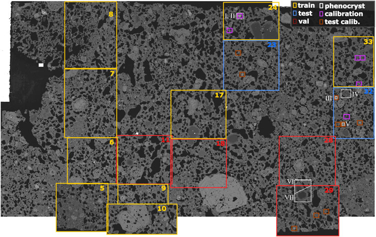
FIGURE 1. BSE map of the entire thin section with selected areas used for training (large yellow frames), testing (blue frames) and validation (red frames). Small purple frames contain areas with olivines used for calibrations of the BSE grey scale against EPMA mg#. These purple frames and small white filled rectangular on a left upper part of the Figure show the size of single EDS-BSE tiles. Numbers show analytical sessions. Olivines presented in this paper are white color contoured and labeled as I, II etc.

One of the most efficient and routine method employed by petrologists to record fine-scale chemical zoning in minerals is the use of grey scale calibrated high-resolution BSE images. The intensity of the backscattered signal depends on the mean atomic number (Z) of the targeted specimen (Goldstein et al., 2018). For example, BSE scans of olivine and pyroxenes (Morgan et al., 2004; Blundy and Cashman, 2008; Martin et al., 2008; Costa and Morgan, 2010; Saunders et al., 2012) show primary variations in the magnesian number mg# [mg# = Mg/(Fe + Mg)]; brighter pixels indicate a higher concentration of Fe), whereas BSE images of plagioclase (Ginibre et al., 2002) demonstrate variations in Anorthite-Albite content [Anorthite content, An# = Ca/(Ca + Na)]; brighter pixels indicate Ca-rich compositions). Using modern field-emission EPMA and depending on the beam conditions (accelerating voltage, current and contrast in atomic number), BSE images can be now acquired with a spatial resolution of 200–300 nm (Armstrong et al., 2013a; Armstrong et al., 2013b).

Subsequent calibration of the grey scale intensities of these high-quality BSE images against quantitative WDS point analyses (expressed e.g., as mg# or An# for respective minerals) provides 1D compositional traverses or 2D quantitative maps with a submicron (100 nm or less) spatial resolution and analytical uncertainty of $<1mol\%$. When applied to diffusion chronometry, such high spatial BSE resolution allows us to simulate a temporal resolution that is better by a factor of 100 (Costa and Morgan, 2010) than what can be achieved by a conventional EPMA analysis (which has an excitation volume never smaller than 1–1.5μm³, (Reed, 2005; Saunders et al., 2014)).

In practice, the selection of individual minerals with interesting zoning patterns (image segmentation) is usually performed by masking tools and/or threshold or watershed methods using commercial or freeware image processing software, with a large proportion of interactive work (e.g. Barraud (2006); Ebel et al. (2016); Zeng et al. (2018)). However, the manual treatment becomes time-consuming when applied to standard thin section areas, and this process is difficult to automate because the distributions of the grey scale intensities of different minerals (especially of solid solutions) in BSE maps usually overlap (Hrstka et al., 2018). In addition, BSE scans often contain numerous artifacts such as charging, surface contamination, and surface damage from sample preparation. In most studies dealing with small sample areas or large areas with reduced resolution, BSE maps are simultaneously acquired along with X-rays maps (EDS or WDS). In this case the task of image pixel classification and segmentation is directly translated into the task of construction of standard phase composition maps (Kotula et al., 2003; Friel and Lyman, 2006), which can be carried out using simple computer scripts (Togami et al., 2000; De Andrade et al., 2006; Muir et al., 2012; Akkaş et al., 2015; Münch et al., 2015; Buse and Kearns, 2018; Higgins et al., 2021; Sheldrake and Higgins, 2021) or stand-alone programs with graphical user interface (Pre’t et al., 2010; Lanari et al., 2014; Chouinard and Donovan, 2015; Liebske, 2015; Zeng et al., 2018; Yasumoto et al., 2018). This approach provides the best and most consistent method of pixel recognition. However, it becomes extremely time-consuming when applied to areas of thin section scale, due to long EDS- or WDS-map acquisition time. A few recent studies presented semi-automated analytical protocols to accurately and efficiently assign mineral (phase) identities (and chemical composition) to image pixels using only selected representative X-ray element intensity maps for calibration (Crapster-Pregont and Ebel, 2020), or X-Ray maps together with BSE grey scale scans parametrized separately for each mineral phase (Willis et al., 2017). Despite progress in facilitating image analysis, these analytical protocols still involved significant amount of time-consuming image pre- and/or post-processing steps.

It has also been shown recently that, as an alternative to traditional thresholding methods, the task of image segmentation can be successfully accomplished by Machine Learning, in particular by Deep Learning (DL) algorithms (Einsle et al., 2018; Volkenandt et al., 2018; Karimpouli and Tahmasebi, 2019; Dong et al., 2020; Lou et al., 2020). For example, Lormand et al. (2018) applied the trainable Weka segmentation (TWS) plugin in the ImageJ software (Abràmoff et al., 2004; Arganda-Carreras et al., 2017) for the sets of BSE images of glassy volcanic shards. In this way, these authors derived a plagioclase crystal segmentation for samples with low crystallinities. However, they also found inconsistent segmentations and failures in crystal boundary recognition in more crystalline samples, most likely due to the insufficient data for training. Since the training data must be generated by the user in a time-consuming interactive process, only a limited number of training examples are available. Even more problematic is that in this way only a part of the variability within the target class is mapped, since e.g., edges can only be captured with difficulty. The generalization behavior of the Fast Forest (FF) (Yates and Islam, 2021) model trained with this data is limited. Therefore manual interaction is obligatory for the application to new data. If sufficient training samples are available, FF and other classical machine learning techniques are outperformed by DL models like convolutional neural networks (CNN) (Le Cun et al., 1989; Krizhevsky et al., 2017) and their variants for pixel-wise classification, especially Fully Convolutional Neural Networks (FCN) (Long et al., 2015). This is thought to be due to the fact that DL methods learn to extract meaningful features from a larger receptive field in the training procedure, whereas traditional classifiers such as FF rely on hand-crafted features that are selected by the user at the beginning and they are not changed in the training process. This problem is aggravated if the hand-crafted features are only based on the pixel intensities, in which case no information of the local pattern of grey values is presented to the classifier. In contrast, DL methods explore all possible features in principle and use the most appropriate ones. However, this theoretical benefit of DL methods always comes at the cost of the requirement of a large amount of training data. Examples of the successful application of DL for the segmentation of electron microscope data can already be found in the literature. Chen et al. (2020) performed data mining on 300 SEM images acquired in secondary electron mode, and a FCN (a modified U-Net architecture (Ronneberger et al., 2015)) was able to effectively separate clay particles from the matrix mineral grains, with pixel grey scale levels that are nearly indistinguishable even for experienced researcher.

In this work we present a framework for such a largescale analysis covering a whole thin section and focusing on olivine crystals in a volcanic rock sample. However, the proposed methodology can be also applied to the analysis of other minerals. Several steps are required to perform this largescale analysis: 1) the identification of relevant areas, in our case the segments in which olivine crystals are present; 2) the data acquisition; and 3) the statistical analysis of the selected areas. All steps have to be automated and in 2) the dependence on time-consuming data acquisition methods has to be minimized. Our framework can be divided in three processing steps:

1) BSE images are automatically segmented into olivine patches using a FCN, which solves a) the identification of relevant areas. 2) Based on the BSE input and the segmentation results from step 1), the mg# is calculated for each pixel using a calibration of BSE intensities against mg# from microprobe data on selected areas (crystals). Applying the calibration leads to the identification of the mg# for each pixel with a quality comparable to the microprobe measurements. The generation of such a huge dataset would be dramatically time consuming when using microprobe measurements due to the long acquisition time. This processing step addresses b), the data acquisition within acceptable time. 3) Finally, a global statistical analysis is carried out. The combination of connected component analysis and estimation of rim to core ratio allows to classify the olivine crystals by their size and zoning characteristics. The respective results are used to tackle c), the automation of the statistical analysis.

The key part of the framework is the semantic segmentation of the olivine crystals. A major difference to the work of Ronneberger et al. (2015) is the automatic generation of a sufficient amount of training examples. We achieve this by using EDS scans acquired simultaneously with BSE. The advantage is that the pixel-wise classification of olivine in EDS scans can easily be done by thresholding the intensity signal values using key chemical elements. These olivine classifications can directly be used as training data for the BSE segmentation. Based on this method we train a model and use it to create a olivine segmentation for an entire thinsection. Subsequently, the segmentation is used for the prediction of the mg# and large-scale analysis of olivine crystals.

3 Methodology and Data

3.1 Dataset Sample

In this study we used a standard thin section (48 × 28 mm² with a sample working area of 40 × 24 mm²) of a high-magnesia basaltic andesite from the Bulochka cinder cone of the Klyuchevskoy volcano, Kamchatka (12% MgO, 52% SiO₂, (Ariskin et al., 1995; Almeev et al., 2013; Portnyagin et al., 2019). The investigated sample is a vesicular basalt with olivine and clinopyroxene phenocrysts with sporadic occurrence of orthopyroxene and rare spinel (which tend to occur as inclusion in olivine). Large phenocrysts of plagioclase are rare; this phase mostly occurs as microphenocryst or in intergrowths with evolved clinopyroxene. The groundmass is composed of olivine, clinopyroxene, plagioclase, Fe-Ti oxides and recrystallized matrix glass. The sample contains the most primitive magnesian clinopyroxene and olivine from the Klyuchevskoy volcano (e.g. mg# = 85–91mol%) and was previously investigated for melt inclusion studies (Mironov et al., 2015; Portnyagin et al., 2019). According to routine point counting methods using an optical microscope (21,000 points), the phase proportions in this sample are as follows (on vesicle-free basis, vesicles are $\sim 20\%$): $\sim 8.5\%$ olivine, $\sim 9\%$ clinopyroxene, $<0.2\%$ orthopyroxene and oxides, 82% groundmass (Almeev et al., 2013).

3.2 Analytical Methods

High quality BSE images of the entire thin section as well as EDS X-ray maps of selected areas within the thin section (Figure 1) were acquired at the Institute of Mineralogy, Leibniz University Hannover (LUH) using a field emission JEOL JSM-7610FPlus electron microscope, equipped with two Bruker XFlash 6|60 large area SDDs. Analytical conditions were as follows: 15kV acceleration voltage, 10 nA probe current, 10 cycles, 16μs dwell time, line average of 15. The size of tiles was chosen to be 512 × 338 pixels, which allowed a spatial resolution of 1 μm for one pixel.

Chemical profiles along selected olivine crystals were obtained using a Cameca SX-100 electron microprobe at the Institute of Mineralogy, LUH. We used an accelerating voltage of 15kV, probe currents of 40 nA and focused beam. The following internal standards were used for Kα line calibration: Mongol olivine standard (Batanova et al., 2019) for Si, Fe and Mg, wollastonite for Ca, and Mn3O4 for Mn. Peak counting times were 10s and background counting times were 5s on each side of the peak. The accuracy and reproducibility of the measurements were controlled by replicated measurements of Mongol (Batanova et al., 2019) and San Carlos (Jarosewich et al., 1980) reference olivines.

3.3 Input Data for the Automatic Analysis

The input data is composed of three subsets dedicated to subtasks of our framework.

DL-Data: consists of corresponding 2400 BSE and EDS tiles and is used for the training, testing and validation of the DL model. Note that the BSE and EDS tiles are pixel-wise aligned due to the sensing setup. Table 1 and Figure 1 show the rectangular areas which were used for the DL training (yellow frames), testing (blue frames) and validation (red frames). The net acquisition time for the DL-Data is ca. 7 days.

TABLE 1

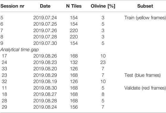
TABLE 1. Analytical subsets (colour frames in Figure 1) used for training, testing and validation.

Calibration-Data: are used for the calibration of the BSE grey intensities against the microprobe data (mg#). The olivines used for the generation of this data are marked with purple (calibrations) and brown (test of calibrations) frames in Figure 1. For this purpose, the data consist of pairs of 1D profiles, a microprobe profile and an extracted BSE profile. BSE profiles are extracted from the BSE images by manually setting the start and end points corresponding to the microprobe profiles.

The acquired accurate microprobe compositional profiles (from rim to rim of the olivine crystals) are used to calculate mg# for further BSE grey scale calibrations.

Thin Section-Data consisting of 9000 BSE tiles are used for statistical treatment and petrological assessments of all olivine crystals in the investigated thin section. This data is visualized by the whole grey value image in Figure 1. The net acquisition time for the Thin Section-Data is ca. 6 days.

3.4 General Task

The overall task is to create a framework which, uses a single channel BSE-image B, and automatically predicts: 1) a 2D binary mask O that indicates which pixel in B corresponds to an olivine crystal (we refer to this task as semantic segmentation); and 2) a two-dimensional map M that contains the corresponding mg# of all pixels in B (we refer to this task as regression). Lastly, there is the task 3) which is to detect complete instances of olivine crystals and typecast (see Table 2) each instance. The predicted mask O as well as the map M should be geometrically aligned with B such that the pixels having the same row and column indices correspond to the same location in the thin section. As shown in the literature, the regression task can be solved by simple parametrization of the BSE grey values against a mineral compositional proxy like mg# (Willis et al., 2017) or An# (Ginibre et al., 2002). The required measurements can e.g., be done by microprobe profiles through entire zoned crystals with subsequent calibration of the BSE grey scale intensity against its mg# for corresponding pixels. This approach, described in Section 4.4, delivers a straightforward solution for the regression task. However, the semantic segmentation task, i.e. the automated pixel-wise binary classification of each pixel in B into the classes olivine and background (non-olivine) is not straightforward, because the same BSE grey values could correspond to both classes. As experts can identify olivine crystals very precisely in BSE-images, we assume that the task is not ill-posed under the consideration of structural information, such as shape or texture. We thus tackle the semantic segmentation by training a convolutional neural network as further described in Section 4.5 Lastly, we exploit the availability of additional sensors, in particular EDS element maps, for the automated generation of the training data. Due to a lower precision (than EPMA), EDS maps are not suited for a pixel-wise analysis of chemical properties such as the mg#, but they contain enough information to automatically generate reference olivine maps to train the segmentation model, which is further elaborated in Section 4.1. The framework is shown in Figure 2.

TABLE 2

TABLE 2. Assignment rules for the automated classification of olivine crystals.

FIGURE 2

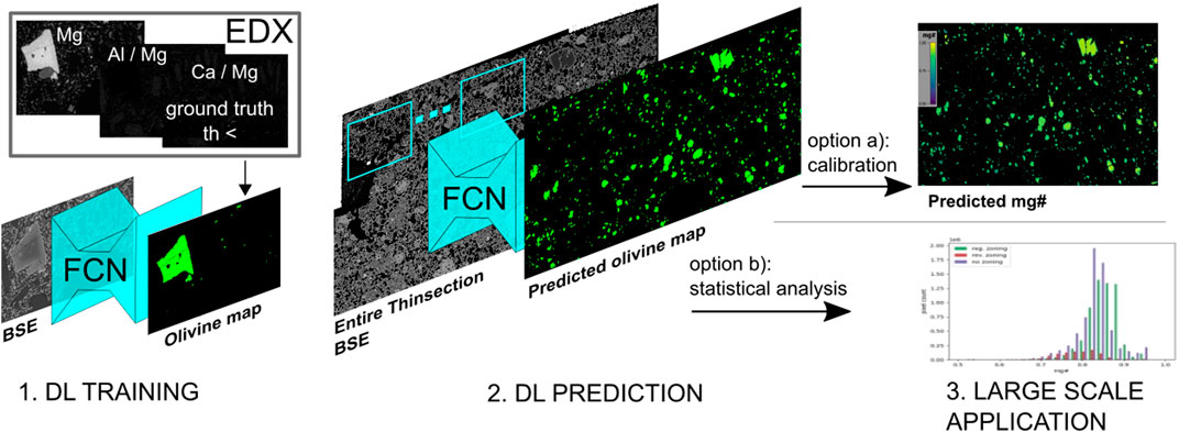
FIGURE 2. Working protocol of the presented method. 1. DL Training: BSE images are used as input and ground truth is generated from EDS data. 2) DL Prediction: Olivine segmentation from BSE image. 3. a) Calibration: Estimation of the relationship between EPMA and BSE values to determine mg#. For the pixels that are classified as Olivine, mg# values are predicted based on regression parameters. 3. b) Statistical analysis based on olivine segmentation.

3.5 Automated Generation of Olivine Maps

Because the semantic segmentation task is tackled using a learning approach, training samples are required. Each sample consists of a BSE image B and the corresponding reference olivine mask O. We propose to generate the reference masks by a pixel-wise rule based classification using the EDS X-Ray intensity criteria (Ca/Mg < 0.1, Al/Mg < 0.1 and Mg > 30) to discriminate olivine and non-olivine pixels in BSE images. As the absolute values for each element measured by the EDS also depend on the analytical mapping settings, the Ca/Mg and Al/Mg ratios are used in addition to the value of total Mg. If Mg = 0 then Ca/Mg is assumed as infinite. A pixel is classified as olivine if all rules hold.

An example of this threshold-based segmentation is shown in Figure 3 B where green pixels represent olivines and black pixels indicate the remaining non-olivine phases. It should be noted that, although in this paper we focus on automated segmentation of olivine crystals, the approach can be easily applied for the classification of other minerals that can be identified based on element ratios. In this way, a large number of training examples (input: BSE and output: olivine map) can be generated, which are used to train the Deep Learning model in the subsequent step.

FIGURE 3

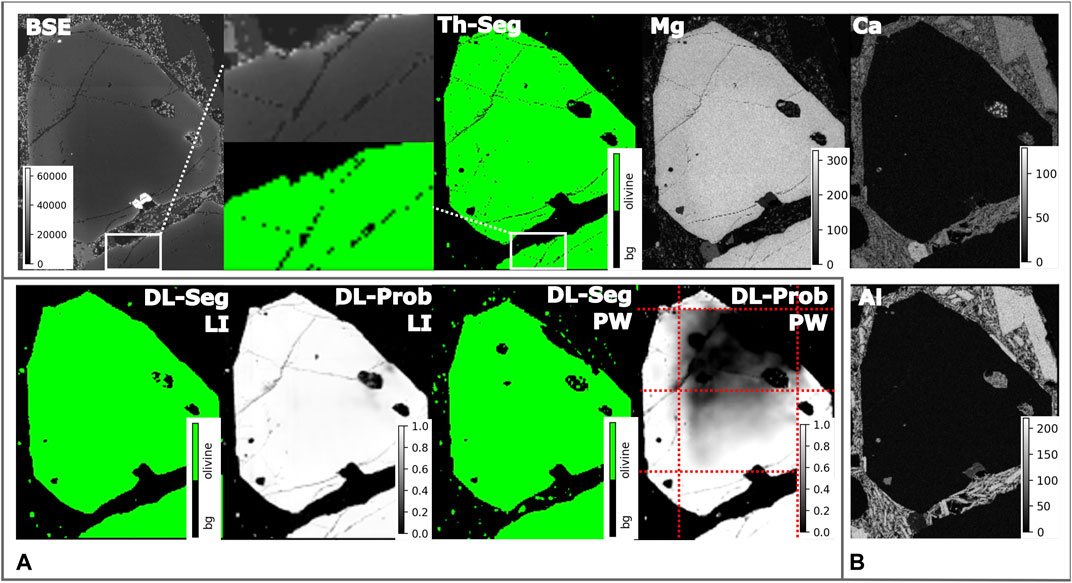
FIGURE 3. This figure shows crystal from the validation part othe DL-Data (Figure 1 VI). Panel (A) presents comparison between DL segmentation using the large image inference method described in Section 3.6.3 (LI) and patch wise segmentation result (PW). The DL-Seg subfigures shows the binary segmentation and the DL-Prob subfigures shows the inference result of the model before the application of the dl_th. Red dashed lines represent the patch borders. Panel (B) is composed of the BSE image and the Ca, Al, Mg X-Ray elemental maps used for the threshold segmentation and the resulting Th-Seg binary segmented olivine map.

3.6 Semantic Segmentation Task

Based on the obtained training data, as described in the previous section, a Fully Convolutional Neural Network (FCN) is trained for the pixel-wise classification. To that end, we rely on a well-known architecture DeepLabV3, shortly described in Section 3.6.1.

3.6.1 Model

The DeepLabV3 architecture used in this paper was originally designed for the pixel-wise classification of street-scenes, but it has been shown to be useful for tasks from other domains like medical image processing (Tang et al., 2018) and remote sensing Niu et al. (2019). We use a network pre-trained on the Common Objects in Context (CoCo) dataset (Lin et al., 2014). This dataset consists of three-channel RGB images of everyday objects and corresponding label maps. It is different from our data, but it allows the network to learn a low-level feature representation that can be reused. Whereas the high-level features may change during the training on our data, the low-level features do not have to be learned again, which enables a more efficient usage of the available data (Yosinski et al., 2014). In our case the inputs of the network are normalized BSE images with only one channel. To be able to feed data into all three input channels of the (pre-trained) network we replicate BSE images three times to artificially adjust the number of channels. The direct output of the model consists of a 2D map of probabilities between 0 and 1 for each pixel to belong to olivine. That is, a probability close to zero indicates that a pixel does not correspond to olivine, whereas a probability close to 1 indicates that a pixel is very likely to belong to olivine. The probabilities are converted into a binary segmentation by applying a threshold (dl_th). $d{l}_{th}\in \mathbb{R}\cap (\mathrm{0,1})$ is a scalar chosen in the interval between 0 and 1.

3.6.2 Training

The network is trained by iteratively minimizing the prediction error starting from a pre-trained state of the network. Particularly, in each iteration a set of images (called a mini-batch) of the training subset are presented to the network which will make a pixel-wise prediction for each image. Then the pixel-wise binary cross-entropy Murphy (2012) between the prediction and the reference is computed, acting as a measure for the difference between the two. In the update step of each iteration the parameters of the network are adjusted according to the negative gradient of the cross-entropy w.r.t. all parameters. This procedure is called Stochastic Gradient Descent (SGD). To be able to analyze the semantic segmentation accuracy and the model, we split the DL-Data into three disjoint subsets—“train”, “test” and “validate” (see Table 1). We use early termination based on the performance of the network on the validation set as measured by the cross-entropy on that set. The original tiles from the analytical sessions (Table 1) are used in training process. In order to avoid overfitting we rely on online data-augmentation, i.e., each training sample is rotated by a random rotation [0°, 90°, 180°, 270°] and flipped horizontally and vertically with a probability of 50%, respectively, before being presented to the network.

3.6.3 Large Image Inference

Our preliminary test has shown that the model performs worse with olivine only partially visible in the input image (cf. Figure 3 A). We assume that this is because the model’s predictions depend on contextual information which is partially missing when predicting close to the image border.

To counteract this effect, we apply two techniques. First, we feed much larger image patches to the network compared to the training stage, which reduces the fraction of pixels that are close to the border of the input image. Second, we perform multiple predictions for same areas in a sliding window approach with overlapping windows. In this way a pixel at the border of one input image will be classified again in an overlapping image, however, this time being in the centre of the image. The analytical sessions which are to be processed in the inference (as listed in Table 1) consist of a certain number of tiles. We perform image stitching based on the tiles to obtain larger, rectangular images SI (ad 1) In general, SI can be used as input to the FCN for segmentation. A FCN consists of a series of sequentially applied convolutions and transposed convolutions. Due to the nature of the (transposed) convolution operation a FCN can be applied to images with an arbitrary size, although practically the input size is limited by the available memory. Therefore we split the large input images into tiles of width LW and height LH pixel. Here, LW and LH are much larger than the size of the tiles used for training. The smaller size of the training tiles is necessary to enable the training on graphics cards, which are often even more limited in operational memory compared to CPUs but capable to highly parallelize the computation which speeds up the training process. The inference can, however, be performed on the CPU as it is far less computationally expensive (ad 2) For the sliding window approach we extend the approach described in Eq. 1 by the overlapping of the tiles. Two horizontally neighbouring LTs are shifted against each other by stride S. We select S always to be far smaller then LW, this results in a overlap of two horizontally neighbouring tiles of LW − S. The vertical dimension is processed analogously. For all LTs from one SI we predict the olivine probabilities per pixel, the direct output of the FCN. Due to overlap there are multiple predicted probabilities for most pixels. These probability values are aggregated by averaging them. To retrieve a binary segmentation we apply the threshold dl_th to the averaged probability values.

3.7 Regression Task

In order to determine the mg# of the predicted olivine pixels, a linear regression is performed based on a set of corresponding BSE intensities and EPMA-determined mg# in selected (predicted) olivines (Figure 1, purple frames). In this way, for each olivine pixel a mg# can be determined, which is a considerable advantage as opposed to EDS measurements, which can only determine individual measurements. Although EPMA measurements are significantly more accurate than e.g., the EDS measurements, EPMA still has two disadvantages. First, it requires an additional instrument and machine time, which affects automation. Second, the EPMA measurements do not fall into the raster of the BSE images acquired on SEM. Therefore an interpolation along the scanning line is required. Although theoretically possible, this step is not yet completely automated and a manual relocation of the microprobe scan-line in the corresponding BSE-images is a prerequisite. We performed a linear regression, which was then evaluated on separate test areas of the thin section using the root mean squared error (RMSE) between the predicted mg# and the one measured by EPMA.

3.8 Outlier Detection

Natural minerals have cracks and holes (vesicles). These artefacts are imaged with varying clarity by different sensors. EDS data show these artefacts less clearly because, despite a nominal resolution of 1μm, the sensor provides information over a larger area. In contrast, a BSE detector has a much higher spatial resolution and its images show the artefacts more clearly (e.g., see Figure 3 B).

The reference segmentation for the DL training process was generated from EDS data and the DeepLabV3 network used is less effective at segmenting small structures such as cracks. Accordingly, in the segmentation results by the DL network, the artefacts are mostly classified as olivines.

To minimize this effect, we applied an algorithm that identifies and removes artefacts, i.e. outliers, based on BSE images. This processing step is necessary in two places. When calibrating the BSE values against mg#, outliers in the BSE data are removed and replaced by linearly interpolated values; when predicting the mg# from the segmented images, the procedure is used for the second time.

The BSE values within the olivines are subject to natural variation. There are continuous changes due to zoning within the crystals and abrupt changes localised at the edge of the crystals. The intensity values in the middle of the artefacts are clearly different from those in the olivine itself. However, the transition to these values is not singular, but often in the form of a continuous gradient. Preliminary investigations have shown that such a progression from the edge to the centre of the artefact can only be poorly identified by a simple procedure such as Z-score (Caouette et al., 1968), as this procedure is based on the statistical distribution of the values and does not take spatial information into account.

The local outlier factor (LOF) (Breunig et al., 2000) algorithm is based on local density of the n-dimensional points, which is determined using a k nearest neighbor algorithm. The local orientation of the LOF algorithm is better suited to identify the artefacts. To generate an input suitable for the LOF algorithm from the BSE image, a 3D feature space is generated with the column and row indices as the first two features and the BSE intensity as the third feature.

3.9 Data Post-processing

As a result of DL segmentation, we obtained a thin section dataset of 9,000 tiles with olivine pixels separated from the remaining matrix. The next step includes automated evaluation of the entire thin section (i.e., not only the coloured frames in Figure 1), where olivine crystals can be distinguished according to their size and type of zoning pattern (based on their mg#). In this study, we define the crystal types as follows: first the crystals are categorised according to their size into Microlites, Microphenocrysts and Phenocrysts. In a last group the Phenocrysts are further divided into three sub-groups according to their zoning pattern: Phenocrysts with a normal zoning, where cores are more magnesian than rims, the Phenocrysts with a reversed zoning pattern, with rims that are more magnesian than cores, and Phenocrysts that do not show chemical gradients.

In order to automatically categorise each detected crystal, we implemented the following processing chain. Based on the binary segmentation map a connected components analysis is carried out. In this step a unique ID number is assigned to all olivine pixels that belong to a connected region. In the further processing steps we assume that each connected component represents one crystal. Based on that mask for each crystal its size is computed by counting the number of pixels.

To distinguish the zoning pattern in phenocrysts, the ratio of the BSE signal between core and rim region is computed. This requires a decision for every pixel of a phenocryst according to whether it belongs to the core or to the rim region. To that end, a distance transformation is carried out. In this step the shortest distance d_i from each pixel i of a crystal to its outline is computed. The result of the distance transformation allows us to separate each crystal into a core and a rim region. Particularly, the core region contains all pixels with d_i > d_max/2, where d_max is the largest distance from each pixel belonging to the same crystal to the corresponding border. The remaining pixels correspond to the rim region. However, we exclude the pixels in the border region with a width of b [px], assuming that those are susceptible to be wrongly classified as olivine pixels due to a noisy predictions of the olivine maps. Consequently, the rim region contains pixels with d_max/2 ≥ d_i > b. Finally, the core to rim ratio r is computed for each phenocryst. The classification rules and the selected thresholds are summarised in Table 2. After all detected crystals were classified, global statistics were obtained (see below). It should be noted that this is a simple approach, and further developments are still required in order to address more complex zoning, e.g., with repetitive (oscillatory) zoning patterns. Sets of crystals classified as no zonning pattern contain many crystals with more complex patterns, like crystals with magnesian cores and rims and iron rich mantle.

4 Experimental Results

4.1 Deep Learning Semantic Segmentation

In this section we present the results of the model with the best test set performance. The model has been trained for 29 epochs. In training process 1,328 unique tiles (before augmentation) has been presented to the network. The training duration has been 8 h using a GeForce GTX TITAN X (GM200) GPU. We applied a threshold dl_th of 0.1 to retrieve a binary segmentation. Preliminary investigations have shown that a value of 0.1 for dl_th parameter leads to better results, especially when predicting BSE images with shifted value ranges. We use overall accuracy (OA, in %) and intersection over union (IoU) as performance metrics to evaluate the accuracy and generalisation of the model. IoU is a measure between 0 and 100% indicating how well the predicted olivine segments fit to the ground truth and OA is the percentage of pixels that were predicted correctly. These metrics are defined and computed as follows:

$OA=\frac{TP+TN}{TP+TN+FP+FN}(1)$

$IoU=\frac{TP}{TP+FP+FN}(2)$

where True-Positive (TP) is the number of correctly identified olivine pixels, True-Negative (TN) is the number of correctly identified non olivine pixels, False-Negative (FN) denotes the number of incorrectly identified non olivine pixels, and False-Positive (FP) indicates the number of incorrectly identified olivine pixels. The positive pixels are such that has been identified by the model as olivine and negative are such pixels that has been identified by the model as background. We comparer the Prediciton of the model to the ground truth (see Section 3.5) and if the prediction matchs the ground truth the pixels are identified as True and therefore as TP and TN. In cases where the prediction didn’t match the ground truth the pixels are assumed as False and therefore as FP and FN. The performance values can be seen in Table 3. For both test and validation sets the IoU is approximately 85% and OA is over 98%.

TABLE 3

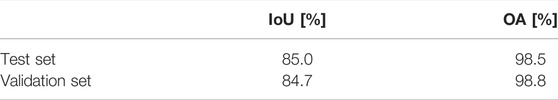
TABLE 3. Performance statistics of the applied DL model.

Figure 4 shows two exemplary results of the DL segmentation in detail. In both cases the model could correctly identify most olivine pixels. The largest error source, however, is a large number of false positive predictions in the area of the crystal rims (red areas in Figure 4). The model tends to overestimate the size of crystals and adds additional olivine pixels to the rim. In addition, false positive predictions can also be observed where the crystal has cracks and holes. However, larger holes as in Figure 4 A are usually correctly classified. In general, the misclassified olivine predictions have a very low probability to belong to an olivine. This can be seen in both Figure 4 (DL-Prob).

FIGURE 4

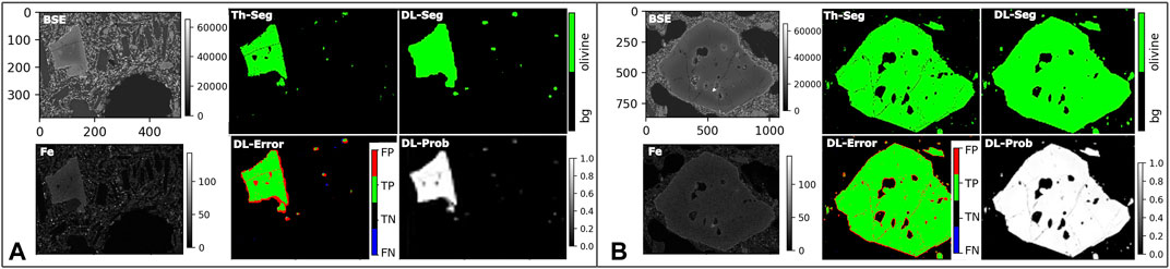
FIGURE 4. Result of the deep learning segmentation. The BSE image is used as input for the semantic segmentation model. For every pixel in the BSE image it is known whether it is olivine or non-olivine (Th-Seg) from to the corresponding EDS maps derived from threshold segmentation (e.g., Table 2). The semantic segmentation produced by DL (DL-Seg) slightly overestimates olivine pixels, mostly at crystal rims (red line in DL-Error). DL-Prob shows probabilities between 0 and 1 of being an olivine pixel predicted by the network. The threshold dl_th is applied to DL-Prob to retrieve DL-Seg. FP-, TP-, TN- and FN- are false positive, true positive, true negative and false negative pixels respectively. The panels (A) and (B) show the result for the crystals III and IV (cf. Figure 1) respectively. The BSE and Fe in the A panel show olivine with almost nested clinopyroxene at the lower end.

It is very important to note that the model is also able to distinguish clinopyroxene and olivine. This can be seen e.g., in Figure 4, where the clinopyroxene subpenocrysts located in the corners of the tile are correctly predicted as non-olivine pixels. These minerals have overlapping BSE grey scale intensities, which is the reason why they cannot be separated by merely thresholding the grey values.

4.2 Variations in Input Data

Both BSE and EDS data can be strongly affected by the instrumental drift which strongly alter the result of regression (see below), and also has a serious effect on correctness of olivine segmentation. Although we used the same EDS mapping settings and also selected the same BSE contrast and brightness, in both cases we observed a shift of the signals between analytical sessions performed with a ∼20 days’ time gap (Table 1). The histograms in Figure 5 show a shift between the intensity of BSE and EDS values. This can cause problems when applying the threshold based approach described in 3.5 and lead to a noisy incomplete ground truth (the false color image in Figure 5 demonstrates the intensity difference between analytical sessions). The DL-Data used in training was created in a shorter period of time, which allowed us to reduce the effect of divergence. Furthermore, the input data is normalized before being feed to the DL model. In addition, DL models are known to be robust against a limited amount of outliers in the training set and is capable to generalize from imperfect data. The FCN trained on the DL-Data predicts olivine with similar accuracy for the default and for the drifted case (Figure 4 DL-Seg A and B). The model only erroneously identifies pixels of small olivine in the last case (Figure 4, DL-Seg B)).

FIGURE 5

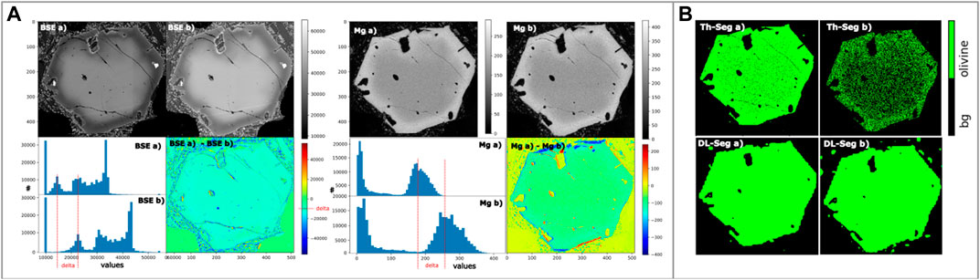
FIGURE 5. Panel (A) Samples I) and II) (cf. Figure 1) depict the same crystal obtained with a $\sim 20$ days time gap. BSE (left A) and EDS X-Ray Mg intensity (right A) signal drift in sessions acquired with 20 days interval (clearly visible in histograms). False-color image show difference between analytical sessions. Panel (B) Threshold segmentation results for 2 analytical sessions (I and II). Despite the difference in input data (intensity), the resulting DL segmentation is comparable (bottom images DL-Seg I) and DL-Seg (B)).

4.3 Outlier Removal

In the next step, outlier olivine pixels are removed. Figure 6 shows BSE image with filtered outliers (red). This is a representative example demonstrating the performance of the algorithm to identify all cracks and holes within the olivine crystal as outlier. Also small olivines next to the phenocryst and the false positive segmented rim are classified as outliers. The remaining few outlier pixels that could not be identified are located at large bubbles and clusters of cracks. Figure 6 shows that the natural zoning profile (green) is preserved while outliers (black) are correctly identified and removed. The points extracted from the filtered profile show low BSE values (see regression in Figure 6).

FIGURE 6

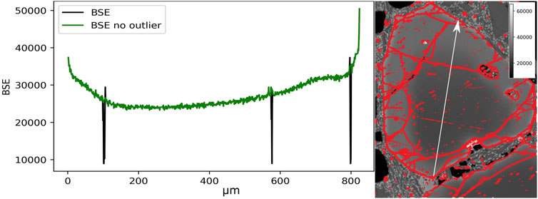
FIGURE 6. The BSE image of zoned olivine crystal (VI cf. Figure 1) with the outliers marked in red and the BSE grey scale intensity profile illustrating the presence of signal outliers (cracks, impurities, holes, surface distractions). The green profile shows filtered data obtained along the white arrow.

4.4 Regression to Determine Mg#

The linear regression of the BSE grey scale intensity against mg# has been performed using the Calibration-Dataset composed of 1,357 olivine pixels. The total range of olivine mg# is within 0.70 and 0.93 in the training data. Only phenocrysts and microphenocrysts were included in Calibration-Data and microlites of olivine present in the matrix were not considered. However, the linear character of the regression allows us to consider that most evolved Fe-rich olivines (which could be potentially under-represented in the training part of Calibration-data) are correctly predicted by extrapolation to mg# lower than 0.7. In future work, a larger compositional range of olivine compositions would be useful. The result of the regression is evaluated using the root mean squared error (RMSE) and coefficient of determination (R²). They are defined in our case as follows. BSE_i and mg#_i are the corresponding BSE intensity value and mg# value with the same index i ∈ [1, N]. Furthermore $\widehat{mg{\#}_i}$ is the predicted mg# with the index i from the BSE_i. The total number of samples is N. Finally the mean mg# is $\overline{mg\#}$. The R² is defined in Eq. 3 and the RMSE is calculated for the predicted and reference mg# is defined in Eq. 4.

$R^2=1-\frac{{\sum }_{i=1}^N{\left(mg{\#}_i-\widehat{mg{\#}_i}\right)}^2}{{\sum }_{i=1}^N{\left(mg{\#}_i-\overline{mg\#}\right)}^2}(3)$

$RMSE=\sqrt{\frac{{\sum }_{i=1}^N{\left(mg{\#}_i-\widehat{mg{\#}_i}\right)}^2}{N}}(4)$

$RMS{E}_{10}=\sqrt{\frac{{\sum }_{i=11}^{N-10}{\left(mg{\#}_i-\widehat{mg{\#}_i}\right)}^2}{N}}(5)$

The RMSE₁₀ of a profile is same as the regular RMSE but without taking in to account the first and last 10 points of a profile, this allows to evaluate the error with reduced influence of the manually registered ends of the profile. The RMSE₁₀ is defined in Eq. 5. In order to investigate the error without the systematic part we define the shifted version of the metrics. We shift the predicted profile along the mg# axis by the RMSE₁₀ to the microprobe reference profile and recalculate the RMSE, in following we refer to it as RMSE_sh for the shifted RMSE and RMSE_sh10 for the shifted RMSE₁₀.

Table 4 and Figure 7 show the difference between the results of the calibration with original BSE data (not filtered) and BSE data after the outlier removal (filtered). The (RMSE) with and without filtering are 0.0045 and 0.0076 respectively. The regression was also tested on the test part of Calibration-Data and resulted with 0.0101 (nonfiltered RMSE) and 0.0097 (filtered RMSE) values. R² of the filtered data is 0.9950 and is slightly better than for not filtered data. The determined function for filtered data is presented in Equation 6:

$\widehat{mg{\#}_i}\left(BS{E}_i\right)=-7.4214BS{E}_i+1.0059(6)$

TABLE 4

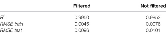
TABLE 4. Performance statistics of the filtered and not filtered calibration.

FIGURE 7

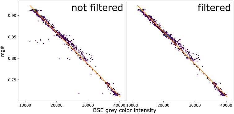
FIGURE 7. Regression task–simple parameterization of the microprobe mg# against SEM BSE grey level intensity performed on the Calibration-Data using selected representative normally and reversely zoned olivines. The calibration lines are shown in orange. On the filtered left image outlier points are visible to the left of the calibration line and on the right image the outliers are removed.

Examples of application of the filtered regression to image tiles with segmented olivine phenocrysts are shown in Figure 8. In Figure 8 A the BSE tile from the validation DL-Data was used in DL training and the resulting mg# profile (red colored line) predicted from the $\widehat{mg{\#}_i}(BS{E}_i)$ function is almost identical to the reference EPMA profile (black) from the microprobe dataset. The RMSE between those two profiles is 0.0064. There are mainly two differences between the predicted mg# and the corresponding reference. The first is that the predicted values have a light scatter around the microprobe mg# profile. The second is the discrepancy at both rims of the olivine crystal. The RMSE₁₀ for the profiles (Figure 8 A) without the first and last 10 values is only 0.0033.

FIGURE 8

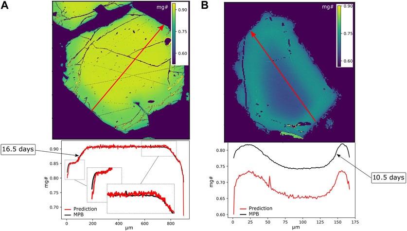
FIGURE 8. Panel (A) Compositional 2D map of mg# in DL-segmented olivine (VII cf. Figure 1) predicted from the BSE grey level. The image tile is from DL-Data and was used in DL training. Red and black lines demonstrate predicted and original (EPMA) mg# profiles. Diffusion modelling along this profile reveals that Fe-Mg exchange occurred for $\sim 16.5$ days, assuming following boundary conditions: T =1200C, 1atm pressure and NNO oxygen buffer, diffusion proceeds along [001] axis (Costa et al., 2008). Panel (B) Compositional 2D map of predicted (from the BSE grey level) mg# in DL-segmented reversely zoned olivine (V cf. Figure 1). The image tile is from the session 32 and was not used in DL training. Red and black lines demonstrate predicted and original (EPMA) mg# profiles. Diffusion modelling along this profile (its right part) revealed that Fe-Mg exchange occurred for 10.5 days, assuming following boundary conditions: T = 1180C, 1atm pressure and NNO oxygen buffer, diffusion proceeds along [010] axis (Costa et al., 2008). The left part of the profile is strongly distorted and cannot be modelled.

The second example in Figure 8 B shows the prediction of the mg# in a 2D (map) and a 1D (profile below) for a reversely zoned olivine in the image tile which was acquired during the session 32. The RMSE between the profiles is 0.0889. If the first and last ten values are ignored RMSE₁₀ is 0.0877. These values represent mainly the shift between the two profiles. The resulting RMSE_sh and RMSE_sh10 are 0.0090 and 0.0053. Similar to the olivine from the session 29, the predicted 1D profile has more noisy patterns and problems at the crystal rims. However, the most fundamental error is caused by a systematic shift of the predicted and observed profiles due to the instrumental drift discussed above.

4.5 Olivine Crystal Segmentation and Classification in Thin Section

In Figure 9 A we present a composite mg# map for the entire thin section with olivines segmented by the DL model. The automated construction of the map using a standard personal computer with 32 GB RAM operational memory, an i5-9600KCPU and a M.2 SSD drive took 16 h. As described in Section 3.6.3, inference for large images uses a larger input size and determines several predictions per pixel. The input size leads to a high demand of operational memory (approx. 128GB) which makes prediction on our GPU impossible and makes it necessary to swap the operational memory to the SSD memory. This combined with the repeated prediction determines the time required for the process. Figure 9 A demonstrates that when the model is trained using in Section 3.6.2 described method (in case of this thin section, about 20% of its area was used in training), the trained model can be used for other thin section BSE maps if BSE intensities of all analytical sessions are corrected against the same references with contrasting grey intensities to remove the instrumental drift. This will dramatically increase the efficiency of studies (e.g., diffusion chronometry) in which a large compositional dataset is necessary to deduce statistical information.

FIGURE 9

FIGURE 9. Panel (A) Composite mg#-in-olivine map for the entire thin section produced from 9000 BSE tiles. Olivine segmentation is performed by DL. Values of mg# are recovered from BSE grey intensities of representative olivines using microprobe compositional data. The original image has a resolution of 1 pixel $\sim 1$ micron and requires 30 Gb of memory. Panel (B) Thin section image with highlighted olivine crystals classified into five groups: microlites (blue color contours), microphenocrysts (magenta), phenocrysts with normal zoning (yellow), phenocrysts with reversed zoning (red) and phenocrysts with no zoning (white). See high resolution image https://www.icaml.org/olmap/.

As a main result of DL olivine segmentation and crystal classification, we present a map of a thin section where all olivine crystals are automatically contoured by different colors depending on the crystal size (area in μm²) and the type of zoning (Figure 9 B). In total, 20,293 micolites (blue contoured areas), 975 microphenocrysts (magenta) and 660 phenocrysts in the entire thin section have been segmented. Among the group of phenocrysts, 124 (yellow), 61 (red) and 475 (white) crystals with normal, reversed and no zoning pattern were classified, respectively (Figure 10 A). As it can be seen in Figure 9 B (see high resolution image https://www.icaml.org/olmap/), the simple criteria (Table 2) proposed in this study for classification of the phenocryst zoning were quite effective to successfully distinguish crystals from the three suggested groups, although some segmentation and classification problems still exist, for example related to broken crystal fragments, mineral inclusions, or olivines with more complex zoning patterns (Figure 10 B-F, see also Discussion below).

FIGURE 10

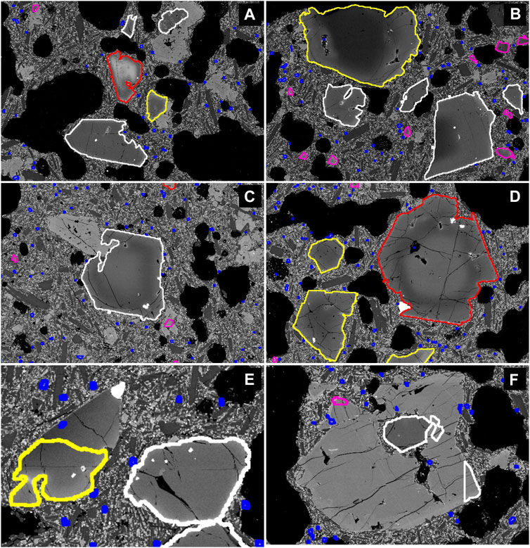
FIGURE 10. Examples of successful (A) and failed automated phenocryst classification (B–D) and olivine DL segmentation (E–F). (A) successful classification of the “normal” (yellow), “reversed” (red) and “no zoning” (white) patterns. The overwhelming majority of the phenocrysts is correctly classified (see full thin section image with segmented olivines here); (B) Two large olivine phenocrysts with normal zoning are classified as “normal” (correct) and “no zoning” (incorrect). The phenocryst with incorrectly recognized zoning pattern in (E) represent a broken fragment (yellow) of a larger crystal; (C) and (D) demonstrate two incorrect cases of classification into “no zoning” (C) and reversed (D) groups for crystals with more complex zoning pattern with iron rich core and rim and more magnesian mantle; (E) olivine phenocryst with normal zoning (yellow) which was only partly recognized as olivine; (F) clinopyroxene phenocryst with areas incorrectly segmented as olivine (small inclusions and triangle-shaped area). See text for details.

5 Discussion

5.1 General Performance of Semantic Segmentation

The presented DL model for the pixel-wise classification of olivine crystals is a nearly perfect tool to distinguish olivine from other mineral phases like plagioclase and clinopyroxene as well as the remaining matrix and holes.

All investigations are performed with data acquired from a single thinsection and therefore there is no information on how well the model performs on data from other thinsection with possible differing background and unseen variations of olivine. The experiments performed here show that the applied FCN model well capable for the segmentation of olivine. Typical features of the crystals such as shape, texture and density variation seem to be sufficient to predict the olivine correctly and also to distinguish it from other phases, despite of overlapping BSE intensity values. The FCN models automatically determines suitable features to perform a good semantic segmentation. These features are encoded in the network and can only be analysed by a human only with difficulties or not at all.

5.1.1 Wrong Pixel Assignments

At the current state, our DL model has a good performance with an IoU value of 85% for the test set and only 1.5–1.2% of erroneously classified pixels (OA: 98.5–98.8%). In a study based on a comparable approach to ours, Chen et al. (2020) achieved an IoU of 0.917 for segmentation of electron microscope data. However, those two values can’t be compared directly, because they represent the performance for different tasks with different properties and challenges. Nevertheless, this shows that the performance achieved with the presented method is close to a state-of-the-art level for electron microscope image segmentation. The model demonstrates the best performance when applied to large phenocrysts. Crystal impurities (holes, inclusions of other phases and cracks) occasionally present in phenocrysts are also identified and segmented successfully. The largest error source is false-positive predictions present at edges of cracks and small structures resulting in a small overestimation of the crystal sizes. These errors are negligible when large olivines are segmented (Figure 4 B), but in the case of smaller crystals they can have a strong negative impact on the predictions (Figure 4 A). This problem can be reduced in future work by applying three approaches: an optimisation of the model parameters i. e., dl_th, using a more suitable model for segmentation of small structures, or improving the quality of the training data. A combination of these measures is also possible. A first solution could be to further optimise the probability threshold for the binary segmentation, as the predicted probabilities are lower for the rim and for the cracks. These errors could be caused or amplified by the up-sampling operation in the DeepLabV3 model that was used. A better alternative could be to use another CNN architecture like HRNet (Wang et al., 2020) which is more suitable to predict small structures. The ground truth generated from EDS element maps, even having a nominal spatial resolution of 1 μm, is in fact characterised by lower spatial resolution when compared to the corresponding BSE tile. This effect can be seen by comparing BSE image (Figure 3 B BSE) and corresponding threshold segmentation (Figure 6 A Th-Seg)). Cracks are less pronounced in the threshold segmentation result than in the BSE image. A pre-processing step could be applied to the training data in order to merge the crack information from the BSE images and the ground truth, i.e. by detecting crack-pixels in the BSE images and not considering these pixels during training.

In order to perform a statistical analysis of the whole thin section we presented an example post-processing step. By applying the trained DL model to the whole thin section, a binary mask was obtained and the regression model was used to predict the mg#for all olivine pixels. Using only expert-knowledge we performed a connected component analysis and a succeeding classification of all crystal instances. Although this approach already results in useful global statistics, there are still some issues which are discussed in the following.

First, the instance segmentation itself may not result in correct instances in all case. If a crystal is separated by a large crack (cf. Figure 5 A, Figure 10 E), this would result in two instances, leading to a wrong interpretation of the size of that crystal and all further derived attributes, e.g. the type. However, in a visual inspection of the instance segmentation, we observed only rarely such a scenario (artificial separation of different crystals due to cracks) and it is not expected to have a large impact on the statistical results in the investigated sample. Nevertheless, this could be improved in further developments.

In addition to systematic errors occurring mostly at olivine boundaries, there are few non-systematic failures in olivine segmentation in areas with a lack of strong BSE gradients in the crystal interior. For example, in Figure 10 E the part of the olivine phenocryst was erroneously not classified as olivine. In addition, in this “non-olivine” area, one microlite was found by the DL model (small blue contoured area). In Figure 10 F, some areas in clinopyroxene phenocrysts were incorrectly classified as olivine (small inclusions and triangular area at the right-bottom side of the crystal). Although such artefacts are extremely rare, a multi class segmentation approach with a dedicated class for clinopyroxene may allow the model to better distinguish between these mineral phases.

5.1.2 Best Model Performance Depends on Input Data

The segmentation model has shown to be robust against constant shifts in the BSE input (cf. Figure 5B). This can be improved e.g., by the extension of the augmentation step with random shift of the BSE input values.

The regression of the mg# is possible with a low error (RMSE = 0.0097 on the test data) and the predicted profiles fit well to the microprobe profiles. The most striking difference is the shift in the profile that sometimes occurs (cf. Figure 8 B). This is caused by the shifts of the BSE image values between different analytical sessions (instrumental drift) and is not a calibration problem. To prevent the BSE and EDS intensity instrumental drift, analytical sessions should be conducted without interruptions. In addition, analytical protocols should include measurements of the standard samples with contrasting BSE intensity at the beginning and at the end of the session.

5.1.3 Uncertainties due to Imperfect Fit Between Pixel Signals Acquired by Different Analytical Instruments

The difference between the RMSE and RMSE₁₀ presented in Section 4.4 shows that the main drawback of the proposed calibration process is the manual assignment of the corresponding BSE intensity (in our case obtained using SEM) and mg# values obtained using the electron microprobe: in our current approach, corresponding pixels have to be assigned manually. In future work, using an automated algorithm to find correspondences between BSE measurements and mg# of arbitrary pixels would allow us to consider a larger amount of data and potentially lead to significant reduction of the errors.

5.2 Crystal Classification

Figure 11 demonstrates an overview of the olivine crystal size distribution obtained for all olivine crystals recovered from the entire thin section. The plot demonstrates that the majority of the crystals $(>80,-,90\%)$ of the phenocryst group range between 10⁴–10⁵ μm² in size and can be confidently distinguished from large phenocrysts with a size of $\sim 10^5-10^6\mu m^2$. Another observation is that almost all olivines with no zoning pattern and reversely zoned olivines range in size between 10⁴–3 × 10⁵ μm². Groups of microlites and microphenocrysts can be confidently separated from each other by a size gap of 500, −,1000 μm². In contrast, the transition between large microphenocrysts and small phenocrysts seems more gradual, and might require consideration of an additional cluster of e.g., subphenocrysts, to separate small microphenocrysts and super large phenocrysts. An expert visual check of the zoning patterns automatically determined within each group of phenocrysts demonstrates that almost all phenocrysts with normal and reversed zoning were correctly identified (see https://www.icaml.org/olmap/with an example of phenocrysts categorized in different groups.). Only three of 124 “normal” phenocrysts were incorrectly determined as “reversed”; however in all three cases they represent broken fragments of initially large crystals (Figure 10 B). Figure 10 C and D. Rare crystals with more complex zoning patterns with iron rich core and rim and more magnesian mantle were classified as “no zoning” and “reversely zoned” crystals. The third group of “no zoning” phenocrysts is more problematic since it contains both crystals with normal and reversed zoning. When compared to the previous two groups, this zoning is weaker, less pronounced but real. It should be noted that in general there are no crystals with complete lack of zoning. Initially it was planned to use this “no zoning” group for a set of phenocrysts with homogeneous interior and very thin iron rich rims formed at the stage of lava cooling after the eruption (quench compositions). However, the results of automated phenocryst classification of the third group demonstrate that the numerical parameters used in this study (e.g., core to rim ratio r) for classification are not accurate to predict such tiny variations in natural zoning pattern and need further improvements. In addition, the current classification approach tries to separate the crystal into a core and a rim area, based on the shortest distance to the boundary of the crystal. However, in the current implementation, holes and cracks inside the crystal are also considered as boundaries, implying that the separation may fail if holes or cracks appear in the central area of the crystal (cf. Figure 4 B). We observed such a situation in some cases, leading to a misclassification of the crystals zoning pattern. This could be improved, e.g., by considering only the external limit of the crystal as boundary. Finally, the current implementation of the connected component analysis and classification is rather slow because it was not optimized yet with respect to the computational efficiency. In the present work, we halved the resolution by removing every second row and column before performing the post-processing, which results in a processing time of 10 h on a regular computer. However, we estimate that after optimization of the implementation, the processing time of the thin section at full resolution could be done in a few hours or even minutes especially when using parallel processing. Future studies may also include considerations of classification of olivine into additional groups such as mineral inclusions, crystal clots and crystal intergrowths.

FIGURE 11

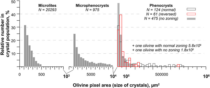
FIGURE 11. Distribution of olivine crystal sizes (pixel area in μm²) in microlite, microphenocryst and phenocryst groups recovered from the entire thin section. See text for details.

5.3 Distribution of Mg# Within Groups and Petrological Interpretations

The full petrological assessment of the results obtained for olivine compositions from different crystal generations cannot be conducted without proper classification of the olivines, which is not yet fully solved at this stage. The main problem is the classification of numerous phenocrysts with weak zoning patterns. Nevertheless, we present a set of histograms (Figure 12) of olivine compositions for four different populations representing phenocrysts with normal zoning, phenocrysts with reversed zoning, microlites and microphenocrysts. An additional population representing phenocrysts with no or little zoning is also given for comparison. Figure 12 shows that almost all crystal populations contain small artificial peaks with high (mg# ∼ 0.94) and low (mg# ∼ 0.54) mg#, indicating cracks and inclusion pixels in olivines, respectively. The presence of such artefacts poses a problem, and the automated detection and elimination of such artefacts needs to be considered in future developments.

FIGURE 12

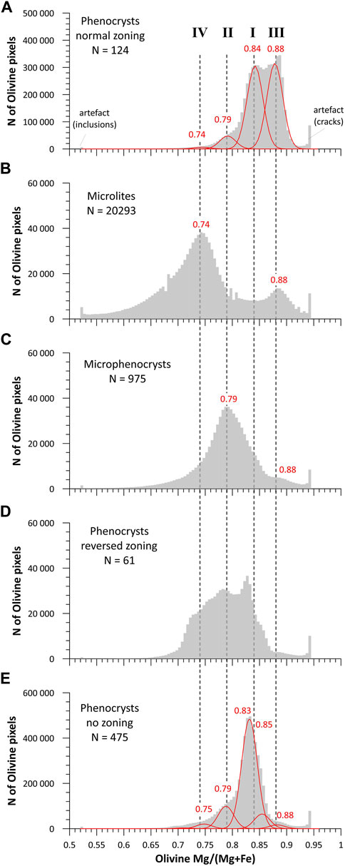
FIGURE 12. Histograms showing distribution of olivine compositions (mg#) for five automatically classified groups: Phenocrysts with normal (A), reversed (D) and “no zoning” (E) zoning, microlites (B) and microphenocrysts (C). Mg# distributions in (A) and (E) were de-convoluted to highlight the presence of hidden compositional populations which exist in all crystal generations. See text for details.

It is out of the scope of this study to discuss in detail the petrological implications of the Machine Learning approach presented here for the magmatic processes at Klyuchevskoy volcano. Here we present briefly possible applications of the data presented in Figure 12. By default phenocrysts represent the earliest and microlites represent the latest crystallization products and should differ in compositions. Thus, with cooling, a magma is expected to have primitive phenocryst cores (with high mg#) and evolved microlites (with lower mg#), but compositions of microlites and phenocryst rims can be more or less identical. The mg# in olivine phenocrysts with normal zoning pattern (Figure 12 A) shows a complex distribution which can result from the overlapping of two major peaks at mg# = 0.88 and 0.84, and two minor peaks at 0.79 and possibly 0.74. The two minor peaks are representative of the rims of the phenocrysts (where compositional zoning is observed). The two major peaks are representative of the core of the zoned phenocrysts and clearly indicate that two populations of olivine were probably affected by the same diffusion process at some stage of the magmatic history. Phenocrysts with mg# = 0.88 may represent a crystal generation from a very primitive magma that mixed with a slightly more evolved reservoir (mg# = 0.84). Note that these highest mg# numbers have been recovered from the few most biggest superphenocrysts. The population of normally zoned phenocrysts composed of olivines with mg# = 0.84 is compositionally similar to the most prominent population of olivines with “no zoning” (Figure 12 E). We interpret this peak at mg# of 0.84 as the composition of the olivines which were formed in the original host “magma” prior to hybridization processes.

The mg# distribution in the microlites has a clear bimodal character with prominent peaks at mg# = 0.88 and 0.74 (Figure 12 B). The microlites have no zoning and, in general, these unzoned microlites are supposed to be the last products crystallizing in the magma and thus represent the last equilibrium stage prior to the eruption. The presence of the two prominent peaks in microlite compositions indicates that the investigated sample results most likely from a mixture of two magmas which contained microlites with different compositions. The microlites with mg# = 0.74 could be formed in an evolved magma stored at shallow level in the plumbing system. The second magma with microlite composition of mg# = 0.88 could be more primitive and was probably stored deeper. Thus, the eruption may have been triggered by the injection of the primitive magma into shallower reservoirs filled with evolved magma. Since microlites with mg# = 0.88 were not re-equilibrated in this new magmatic environment to more iron rich compositions, the mixing event was probably immediately followed by subsequent ascent and eruption.

Although reversely zoned crystals are confidently classified (Figure 12 D), the interpretation of the mg# distribution is complex. This is not surprising, since the shape of these crystals (irregular crystal shapes with extensive resorptions and embayments) and the presence of numerous patchy zones within a more general reversed zoning pattern indicate that these crystals record complex re-equilibration history from evolved (perhaps at mg# = 0.74) towards more primitive compositions during magma replenishments preceeding the final mixing that triggered the eruption.

Finally, in addition to the identification of different populations within one single phase, the automated processing of the zoned olivine crystals provides a unique opportunity to understand magma mixing processes, to constrain thermal evolution of magmas, and to extract time scales of geological processes by applying diffusion chronometry on zoned crystals.

5.4 Olivine Crystal Curating and Catalogue With Different Groups

The automated processing of the olivine crystals (including size, and composition) presented in this study is an ideal tool to characterise quickly and extract high quality 2D textural and compositional information from a whole thin section. However, in addition to this mapping facility, all olivines are separated and classified and each crystal can be individually curated, since it has an unique ID number, providing an excellent archive that can be easily used by other scientists. In https://www.icaml.org/olmap/ we present an example of images, where classified olivines are presented for each group in separate folders. The distribution of the mg# number can be also automatically provided for each olivine.

6 Conclusion and Future Work

In this work fully convolutional neural networks were used to characterize thin sections of volcanic rocks. It has been shown that a model (DeepLabV3) designed for segmentation of RGB images can be used to segment back-scattered electron images of thin sections from volcanic rocks composed of phenocrysts and partly microcrystalline vesicular matrix. The requirement for a large amount of training samples for the training of the CNN has been solved by an automated generation of reference data. The resulting model was found to be successful when applying it to an unknown test dataset. All investigations were performed using a single thin section, therefore future investigations would profit from testing additional samples. The results presented for olivine can be extended to other minerals using a similar approach. A DL model based instance segmentation, i.e., a segmentation that also identifies individual instances of olivine crystals, can offer the opportunity to calculate a large number of statistical features.

The example selected for this study is not an exception but is rather representative of typical lavas from subduction-related volcanoes. It clearly shows that Machine Learning approaches are extremely useful to decode the multiple and complex information that is stored in crystal-bearing lavas. A significant part of the information stored by mineral phases would be definitely unexploited if a simple approach based on a manual selection of a few mineral of interest would have been applied. By analyzing several selected thin sections with the approach presented in this study, samples collected along geological profiles (e.g., drill cores) would provide extremely useful information on temporal and spacial evolutions of volcanic rocks with a considerably reduced man-power and an unprecedented high resolution.

Data Availability Statement

The raw data supporting the conclusion of this article will be made available by the authors, without undue reservation.

Author Contributions

All authors were actively involved in this project, and participated in writing and editing of the presented manuscript. AL, as first author, carried major workload on implementation of the approach, execution of the experiments and writing of the manuscript. RA supervised the acquisition of the used data, is responsible for the development of the automatic training data generation and for the evaluation of the analytical results. DW is responsible for the data post processing development and participated the implementation of the presented approach. PB performed the data acquisition and preliminary data analysis. FR, FH, and MS are responsible for the conceptual development of the approach and the discussion of the results. All authors have (co-)edited corresponding parts of the manuscript.

Conflict of Interest

The authors declare that the research was conducted in the absence of any commercial or financial relationships that could be construed as a potential conflict of interest.

Publisher’s Note

All claims expressed in this article are solely those of the authors and do not necessarily represent those of their affiliated organizations, or those of the publisher, the editors and the reviewers. Any product that may be evaluated in this article, or claim that may be made by its manufacturer, is not guaranteed or endorsed by the publisher.

Acknowledgments

This work has been conducted in the frame of the Forschungsgruppe FOR 2881 “Diffusion chronometry of magmatic systems” funded by the German Science Foundation (DFG). Discussions and comments by S. Chakraborty as well as comments and reviews by AE DP, AB, and MR greatly improved this study and manuscript. M. Oeser is thanked for his help with diffusion modeling.

Footnotes

¹wt%: weight percent

References

Abràmoff, M. D., Magalhães, P. J., and Ram, S. J. (2004). Image Processing with Imagej. Biophotonics Int. 11, 36–42.

Google Scholar

Akkaş, E., Akin, L., Evren Çubukçu, H., and Artuner, H. (2015). Application of Decision Tree Algorithm for Classification and Identification of Natural Minerals Using Sem–Eds. Comput. Geosciences 80, 38–48. doi:10.1016/j.cageo.2015.03.015

CrossRef Full Text | Google Scholar

Albert, H., Costa, F., and Martí, J. (2015). Timing of Magmatic Processes and Unrest Associated with Mafic Historical Monogenetic Eruptions in Tenerife Island. J. Petrol. 56, 1945–1966. doi:10.1093/petrology/egv058

CrossRef Full Text | Google Scholar

Almeev, R. R., Kimura, J.-I., Ariskin, A. A., and Ozerov, A. Y. (2013). Decoding crystal Fractionation in Calc-Alkaline Magmas from the Bezymianny Volcano (Kamchatka, russia) Using mineral and Bulk Rock Compositions. J. Volcanology Geothermal Res. 263, 141–171. doi:10.1016/j.jvolgeores.2013.01.003

CrossRef Full Text | Google Scholar

Arganda-Carreras, I., Kaynig, V., Rueden, C., Eliceiri, K. W., Schindelin, J., Cardona, A., et al. (2017). Trainable Weka Segmentation: a Machine Learning Tool for Microscopy Pixel Classification. Bioinformatics 33, 2424–2426. doi:10.1093/bioinformatics/btx180

PubMed Abstract | CrossRef Full Text | Google Scholar

Ariskin, A., Barmina, G., Ozerov, A. Y., and Nielsen, R. (1995). Genesis of High-Alumina Basalts from Klyuchevskoi Volcano. Petrology 3, 449–472.

Google Scholar

Armstrong, J. T., McSwiggen, P., and Nielsen, C. (2013a). A Thermal Field Emission Electron Probe Microanalyzer for Improved Analytical Spatial Resolution. Microscopy and Analysis 27, 18–22.

Google Scholar

Armstrong, J. T., McSwiggen, P., and Nielsen, C. (2013b). Bridging the Gap Between EPMA and AEM: The Performance of High Resolution Field-Emission Electron Microprobes in the Analysis of Geological Materials. Microscopy and Microanalysis 19, 1254–1255.

CrossRef Full Text | Google Scholar

Barraud, J. (2006). The Use of Watershed Segmentation and Gis Software for Textural Analysis of Thin Sections. J. Volcanology Geothermal Res. 154, 17–33. doi:10.1016/j.jvolgeores.2005.09.017

CrossRef Full Text | Google Scholar

Batanova, V. G., Thompson, J. M., Danyushevsky, L. V., Portnyagin, M. V., Garbe‐Schönberg, D., Hauri, E., et al. (2019). New Olivine Reference Material for In Situ Microanalysis. Geostand Geoanal Res. 43, 453–473. doi:10.1111/ggr.12266

CrossRef Full Text | Google Scholar

Blundy, J., and Cashman, K. (2008). Petrologic Reconstruction of Magmatic System Variables and Processes. Rev. Mineralogy Geochem. 69, 179–239. doi:10.2138/rmg.2008.69.6

CrossRef Full Text | Google Scholar

Breunig, M. M., Kriegel, H.-P., Ng, R. T., and Sander, J. (2000). “Lof,” in SIGMOD ’00: Proceedings of the 2000 ACM SIGMOD International Conference on Management of Data (New York, NY, USA: Association for Computing Machinery), 93–104. doi:10.1145/342009.335388

CrossRef Full Text | Google Scholar

Buse, B., and Kearns, S. (2018). Evaluating X-ray Microanalysis Phase Maps Using Principal Component Analysis. Microsc. Microanal 24, 116–125. doi:10.1017/S1431927618000090

PubMed Abstract | CrossRef Full Text | Google Scholar

Caouette, J. B., Altman, E. I., Narayanan, P., and Altman, Z. (1968). 1.6 Z-Score Estimated for Non-manufacturers & Emerging Markets. Altman Z-Score 189, 1.

Google Scholar

Cashman, K., and Blundy, J. (2013). Petrological Cannibalism: the Chemical and Textural Consequences of Incremental Magma Body Growth. Contrib. Mineral. Petrol. 166, 703–729. doi:10.1007/s00410-013-0895-0

CrossRef Full Text | Google Scholar

Chakraborty, S. (2008). Diffusion in Solid Silicates: A Tool to Track Timescales of Processes Comes of Age. Annu. Rev. Earth Planet. Sci. 36, 153–190. doi:10.1146/annurev.earth.36.031207.124125

CrossRef Full Text | Google Scholar

Chen, Z., Liu, X., Yang, J., Little, E., and Zhou, Y. (2020). Deep Learning-Based Method for Sem Image Segmentation in mineral Characterization, an Example from Duvernay Shale Samples in Western canada Sedimentary basin. Comput. Geosciences 138, 104450. doi:10.1016/j.cageo.2020.104450

CrossRef Full Text | Google Scholar

Cheng, G., and Guo, W. (2017). Rock Images Classification by Using Deep Convolution Neural Network. J. Phys. Conf. Ser. 887, 012089. doi:10.1088/1742-6596/887/1/012089

CrossRef Full Text | Google Scholar

Chouinard, J., and Donovan, J. (2015). Quantitative Elemental Mapping with Electron Microprobe and Automated Data Analysis. Microsc. Microanal 21, 2193–2194. doi:10.1017/S1431927615011745

CrossRef Full Text | Google Scholar

Costa, F., Dohmen, R., and Chakraborty, S. (2008). Time Scales of Magmatic Processes from Modeling the Zoning Patterns of Crystals. Rev. Mineralogy Geochem. 69, 545–594. doi:10.2138/rmg.2008.69.14

CrossRef Full Text | Google Scholar

Costa, F., and Morgan, D. (2010). Time Constraints from Chemical Equilibration in Magmatic Crystals. Hoboken, NJ, USA: John Wiley I& Sons, Ltd, 125–159. chap. 7. doi:10.1002/9781444328509.ch7

CrossRef Full Text | Google Scholar

Costa, F., Shea, T., and Ubide, T. (2020). Diffusion Chronometry and the Timescales of Magmatic Processes. Nat. Rev. Earth Environ. 1, 201–214. doi:10.1038/s43017-020-0038-x

CrossRef Full Text | Google Scholar

Crapster-Pregont, E. J., and Ebel, D. S. (2020). Reducing Supervision of Quantitative Image Analysis of Meteorite Samples. Microsc. Microanal 26, 63–75. doi:10.1017/S1431927619015216

PubMed Abstract | CrossRef Full Text | Google Scholar

Davidson, J. P., Morgan, D. J., Charlier, B. L. A., Harlou, R., and Hora, J. M. (2007). Microsampling and Isotopic Analysis of Igneous Rocks: Implications for the Study of Magmatic Systems. Annu. Rev. Earth Planet. Sci. 35, 273–311. doi:10.1146/annurev.earth.35.031306.140211

CrossRef Full Text | Google Scholar

De Andrade, V., Vidal, O., Lewin, E., O'Brien, P., and Agard, P. (2006). Quantification of Electron Microprobe Compositional Maps of Rock Thin Sections: an Optimized Method and Examples. J. Metamorphic Geology. 24, 655–668. doi:10.1111/j.1525-1314.2006.00660.x

CrossRef Full Text | Google Scholar

de Maisonneuve, C. B., Costa, F., Huber, C., Vonlanthen, P., Bachmann, O., and Dungan, M. A. (2016). How Do Olivines Record Magmatic Events? Insights from Major and Trace Element Zoning. Contrib. Mineral. Petrol. 171, 1–20. doi:10.1007/s00410-016-1264-6

CrossRef Full Text | Google Scholar

Dong, P., Provencher, B., Basim, N., Piché, N., and Marsh, M. (2020). Forget about Cleaning up Your Micrographs: Deep Learning Segmentation Is Robust to Image Artifacts. Microsc. Microanal 26, 1468–1469. doi:10.1017/s1431927620018231

CrossRef Full Text | Google Scholar

Ebel, D. S., Brunner, C., Konrad, K., Leftwich, K., Erb, I., Lu, M., et al. (2016). Abundance, Major Element Composition and Size of Components and Matrix in Cv, Co and Acfer 094 Chondrites. Geochimica et Cosmochimica Acta 172, 322–356. doi:10.1016/j.gca.2015.10.007

CrossRef Full Text | Google Scholar

Einsle, J. F., Martineau, B., Buisman, I., Vukmanovic, Z., Johnstone, D., Eggeman, A., et al. (2018). All Mixed up: Using Machine Learning to Address Heterogeneity in (Natural) Materials. Microsc. Microanal 24, 562–563. doi:10.1017/S1431927618003306

CrossRef Full Text | Google Scholar

Friel, J. J., and Lyman, C. E. (2006). Tutorial Review: X-ray Mapping in Electron-Beam Instruments. Microsc. Microanal. 12, 2–25. doi:10.1017/S1431927606060211

PubMed Abstract | CrossRef Full Text | Google Scholar

Ginibre, C., Kronz, A., and Wörner, G. (2002). High-resolution Quantitative Imaging of Plagioclase Composition Using Accumulated Backscattered Electron Images: New Constraints on Oscillatory Zoning. Contrib. Mineral. Petrol. 142, 436–448. doi:10.1007/s004100100298

CrossRef Full Text | Google Scholar

[Dataset] Goldstein, J. I., Newbury, D. E., and Michael, J. R. (2018). Scanning Electron Microscopy and X-ray Microanalysis. Berlin, Germany: Springer.

Google Scholar

Higgins, O., Sheldrake, T., and Caricchi, L. (2021). Quantitative Chemical Mapping of Plagioclase as a Tool for the Interpretation of Volcanic Stratigraphy: an Example from Saint Kitts, Lesser Antilles. Bull. volcanology 83, 1–15. doi:10.1007/s00445-021-01476-x

CrossRef Full Text | Google Scholar

Hrstka, T., Gottlieb, P., Skála, R., Breiter, K., and Motl, D. (2018). Automated Mineralogy and Petrology - Applications of Tescan Integrated mineral Analyzer (Tima). J. Geosci. 63, 47–63. doi:10.3190/jgeosci.250

CrossRef Full Text | Google Scholar

Jarosewich, E., Nelen, J. A., and Norberg, J. A. (1980). Reference Samples for Electron Microprobe Analysis*. Geostandards Newsl. 4, 43–47. doi:10.1111/j.1751-908X.1980.tb00273.x

CrossRef Full Text | Google Scholar

Kahl, M., Chakraborty, S., Costa, F., and Pompilio, M. (2011). Dynamic Plumbing System beneath Volcanoes Revealed by Kinetic Modeling, and the Connection to Monitoring Data: An Example from Mt. etna. Earth Planet. Sci. Lett. 308, 11–22. doi:10.1016/j.epsl.2011.05.008

CrossRef Full Text | Google Scholar

Kahl, M., Chakraborty, S., Costa, F., Pompilio, M., Liuzzo, M., and Viccaro, M. (2013). Compositionally Zoned Crystals and Real-Time Degassing Data Reveal Changes in Magma Transfer Dynamics during the 2006 summit Eruptive Episodes of Mt. etna. Bull. Volcanol 75, 1–14. doi:10.1007/s00445-013-0692-7

CrossRef Full Text | Google Scholar

Kahl, M., Viccaro, M., Ubide, T., Morgan, D. J., and Dingwell, D. B. (2017). A Branched Magma Feeder System during the 1669 Eruption of Mt Etna: Evidence from a Time-Integrated Study of Zoned Olivine Phenocryst Populations. J. Petrol. 58, 443–472. doi:10.1093/petrology/egx022

CrossRef Full Text | Google Scholar

Karimpouli, S., and Tahmasebi, P. (2019). Segmentation of Digital Rock Images Using Deep Convolutional Autoencoder Networks. Comput. Geosciences 126, 142–150. doi:10.1016/j.cageo.2019.02.003

CrossRef Full Text | Google Scholar

Kotula, P. G., Keenan, M. R., and Michael, J. R. (2003). Automated Analysis of Sem X-ray Spectral Images: A Powerful New Microanalysis Tool. Microsc. Microanal 9, 1–17. doi:10.1017/S1431927603030058

CrossRef Full Text | Google Scholar

Krizhevsky, A., Sutskever, I., and Hinton, G. E. (2017). Imagenet Classification with Deep Convolutional Neural Networks. Commun. ACM 60, 84–90. doi:10.1145/3065386

CrossRef Full Text | Google Scholar

Lanari, P., Vidal, O., De Andrade, V., Dubacq, B., Lewin, E., Grosch, E. G., et al. (2014). XMapTools: A MATLAB-Based Program for Electron Microprobe X-ray Image Processing and Geothermobarometry. Comput. Geosciences 62, 227–240. doi:10.1016/j.cageo.2013.08.010

CrossRef Full Text | Google Scholar

Le Cun, Y., Boser, B., Denker, J. S., Henderson, D., Howard, R. E., Hubbard, W., et al. (1989). “Handwritten Digit Recognition with a Back-Propagation Network,” in NIPS’89: Proceedings of the 2nd International Conference on Neural Information Processing Systems (Cambridge, MA, USA: MIT Press), 396–404.

Google Scholar

Liebske, C. (2015). iSpectra: An Open Source Toolbox for the Analysis of Spectral Images Recorded on Scanning Electron Microscopes. Microsc. Microanal 21, 1006–1016. doi:10.1017/S1431927615014336

PubMed Abstract | CrossRef Full Text | Google Scholar

Lin, T.-Y., Maire, M., Belongie, S., Hays, J., Perona, P., Ramanan, D., et al. (2014). “Microsoft Coco: Common Objects in Context,” in European conference on computer vision (Berlin, Germany: Springer), 740–755. doi:10.1007/978-3-319-10602-1_48

CrossRef Full Text | Google Scholar

Long, J., Shelhamer, E., and Darrell, T. (2015). “Fully Convolutional Networks for Semantic Segmentation,” in Proceedings of the IEEE Conference on Computer Vision and Pattern Recognition (CVPR). doi:10.1109/cvpr.2015.7298965

CrossRef Full Text | Google Scholar

Lormand, C., Zellmer, G. F., Németh, K., Kilgour, G., Mead, S., Palmer, A. S., et al. (2018). Weka Trainable Segmentation Plugin in Imagej: A Semi-automatic Tool Applied to crystal Size Distributions of Microlites in Volcanic Rocks. Microsc. Microanal 24, 667–675. doi:10.1017/S1431927618015428

PubMed Abstract | CrossRef Full Text | Google Scholar

Lou, W., Zhang, D., and Bayless, R. C. (2020). Review of mineral Recognition and its Future. Appl. Geochem. 122, 104727. doi:10.1016/j.apgeochem.2020.104727

CrossRef Full Text | Google Scholar

Martin, V. M., Morgan, D. J., Jerram, D. A., Caddick, M. J., Prior, D. J., and Davidson, J. P. (2008). Bang! Month-Scale Eruption Triggering at Santorini Volcano. Science 321, 1178. doi:10.1126/science.1159584

PubMed Abstract | CrossRef Full Text | Google Scholar

Mironov, N., Portnyagin, M., Botcharnikov, R., Gurenko, A., Hoernle, K., and Holtz, F. (2015). Quantification of the CO 2 Budget and H 2 O-CO 2 Systematics in Subduction-Zone Magmas through the Experimental Hydration of Melt Inclusions in Olivine at High H 2 O Pressure. Earth Planet. Sci. Lett. 425, 1–11. doi:10.1016/j.epsl.2015.05.043

CrossRef Full Text | Google Scholar

Morgan, D. J., Blake, S., Rogers, N. W., DeVivo, B., Rolandi, G., Macdonald, R., et al. (2004). Time Scales of crystal Residence and Magma Chamber Volume from Modelling of Diffusion Profiles in Phenocrysts: Vesuvius 1944. Earth Planet. Sci. Lett. 222, 933–946. doi:10.1016/j.epsl.2004.03.030

CrossRef Full Text | Google Scholar

Muir, D. D., Blundy, J. D., and Rust, A. C. (2012). Multiphase Petrography of Volcanic Rocks Using Element Maps: a Method Applied to Mount St. Helens, 1980-2005. Bull. Volcanol 74, 1101–1120. doi:10.1007/s00445-012-0586-0

CrossRef Full Text | Google Scholar

Münch, B., Martin, L. H. J., and Leemann, A. (2015). Segmentation of Elemental Eds Maps by Means of Multiple Clustering Combined with Phase Identification. J. Microsc. 260, 411–426. doi:10.1111/jmi.12309

PubMed Abstract | CrossRef Full Text | Google Scholar

Murphy, K. P. (2012). Machine Learning: A Probabilistic Perspective. Cambridge, MA, USA: MIT press.

Google Scholar

Niu, Z., Liu, W., Zhao, J., and Jiang, G. (2019). Deeplab-based Spatial Feature Extraction for Hyperspectral Image Classification. IEEE Geosci. Remote Sensing Lett. 16, 251–255. doi:10.1109/LGRS.2018.2871507

CrossRef Full Text | Google Scholar

Portnyagin, M., Mironov, N., Botcharnikov, R., Gurenko, A., Almeev, R. R., Luft, C., et al. (2019). Dehydration of Melt Inclusions in Olivine and Implications for the Origin of Silica-Undersaturated Island-Arc Melts. Earth Planet. Sci. Lett. 517, 95–105. doi:10.1016/j.epsl.2019.04.021

CrossRef Full Text | Google Scholar

Pret, D., Sammartino, S., Beaufort, D., Meunier, A., Fialin, M., and Michot, L. J. (2010). A New Method for Quantitative Petrography Based on Image Processing of Chemical Element Maps: Part I. Mineral Mapping Applied to Compacted Bentonites. Am. Mineral. 95, 1379–1388. doi:10.2138/am.2010.3431

CrossRef Full Text | Google Scholar

Putirka, K. D. (2008). Thermometers and Barometers for Volcanic Systems. Rev. Mineralogy Geochem. 69, 61–120. doi:10.2138/rmg.2008.69.3

CrossRef Full Text | Google Scholar

Reed, S. J. B. (2005). Electron Microprobe Analysis and Scanning Electron Microscopy in Geology. Cambridge, MA, USA: Cambridge University Press.

Google Scholar

Ronneberger, O., Fischer, P., and Brox, T. (2015). “U-net: Convolutional Networks for Biomedical Image Segmentation,” in International Conference on Medical image computing and computer-assisted intervention (Berlin, Germany: Springer), 234–241. doi:10.1007/978-3-319-24574-4_28

CrossRef Full Text | Google Scholar

Ruth, D. C. S., Costa, F., Bouvet de Maisonneuve, C., Franco, L., Cortés, J. A., and Calder, E. S. (2018). Crystal and Melt Inclusion Timescales Reveal the Evolution of Magma Migration before Eruption. Nat. Commun. 9, 1–9. doi:10.1038/s41467-018-05086-8

PubMed Abstract | CrossRef Full Text | Google Scholar

Saunders, K., Blundy, J., Dohmen, R., and Cashman, K. (2012). Linking Petrology and Seismology at an Active Volcano. Science 336, 1023–1027. doi:10.1126/science.1220066

PubMed Abstract | CrossRef Full Text | Google Scholar

Saunders, K., Buse, B., Kilburn, M. R., Kearns, S., and Blundy, J. (2014). Nanoscale Characterisation of crystal Zoning. Chem. Geology. 364, 20–32. doi:10.1016/j.chemgeo.2013.11.019

CrossRef Full Text | Google Scholar

Seddio, S. M., and Donovan, J. J. (2016). Comparing the Intensities and Spectral Resolution Achieved by Wavelength-Dispersive Spectrometers on Microprobes and Sems. Microsc. Microanal 22, 444–445. doi:10.1017/S143192761600307X

CrossRef Full Text | Google Scholar

Shea, T., Costa, F., Krimer, D., and Hammer, J. E. (2015). Accuracy of Timescales Retrieved from Diffusion Modeling in Olivine: A 3d Perspective. Am. Mineral. 100, 2026–2042. doi:10.2138/am-2015-5163

CrossRef Full Text | Google Scholar

Sheldrake, T., and Higgins, O. (2021). Classification, Segmentation and Correlation of Zoned Minerals. Comput. Geosciences 156, 104876. doi:10.1016/j.cageo.2021.104876

CrossRef Full Text | Google Scholar

Streck, M. J. (2008). Mineral Textures and Zoning as Evidence for Open System Processes. Rev. Mineralogy Geochem. 69, 595–622. doi:10.2138/rmg.2008.69.15

CrossRef Full Text | Google Scholar

Tang, W., Zou, D., Yang, S., and Shi, J. (2018). “Dsl: Automatic Liver Segmentation with Faster R-Cnn and Deeplab,” in International Conference on Artificial Neural Networks (Berlin, Germany: Springer), 137–147. doi:10.1007/978-3-030-01421-6_14

CrossRef Full Text | Google Scholar

Togami, S., Takano, M., Kumazawa, M., and Michibayashi, K. (2000). An Algorithm for the Transformation of XRF Images into Mineral-Distribution Maps. Can. Mineral. 38, 1283–1294. doi:10.2113/gscanmin.38.5.1283

CrossRef Full Text | Google Scholar

Volkenandt, T., Freitag, S., and Rauscher, M. (2018). Machine Learning Powered Image Segmentation. Microsc. Microanal 24, 520–521. doi:10.1017/S1431927618003094

CrossRef Full Text | Google Scholar

Wang, J., Sun, K., Cheng, T., Jiang, B., Deng, C., Zhao, Y., et al. (2021). Deep High-Resolution Representation Learning for Visual Recognition. IEEE Trans. Pattern Anal. Mach. Intell. 43, 3349–3364. doi:10.1109/TPAMI.2020.2983686

PubMed Abstract | CrossRef Full Text | Google Scholar

Willis, K. V., Srogi, L., Lutz, T., Monson, F. C., and Pollock, M. (2017). Phase Composition Maps Integrate mineral Compositions with Rock Textures from the Micro-meter to the Thin Section Scale. Comput. Geosciences 109, 162–177. doi:10.1016/j.cageo.2017.08.009

CrossRef Full Text | Google Scholar

Yasumoto, A., Yoshida, K., Kuwatani, T., Nakamura, D., Svojtka, M., and Hirajima, T. (2018). A Rapid and Precise Quantitative Electron Probe Chemical Mapping Technique and its Application to an Ultrahigh-Pressure Eclogite from the Moldanubian Zone of the Bohemian Massif (Nové Dvory, Czech Republic). Am. Mineral. 103, 1690–1698. doi:10.2138/am-2018-6323CCBY

CrossRef Full Text | Google Scholar

Yates, D., and Islam, M. Z. (2021). Fastforest: Increasing Random forest Processing Speed while Maintaining Accuracy. Inf. Sci. 557, 130–152. doi:10.1016/j.ins.2020.12.067

CrossRef Full Text | Google Scholar

Yosinski, J., Clune, J., Bengio, Y., and Lipson, H. (2014). How Transferable Are Features in Deep Neural Networks? CoRR abs/1411.1792.

Google Scholar

Zeng, L., Cheng, L., Costa, F., and Herrin, J. (2018). Cemin: A Matlab-Based Software for Computational Phenocryst Extraction and Statistical Petrology. Geochem. Geophys. Geosyst. 19, 1378–1392. doi:10.1002/2017gc007346

CrossRef Full Text | Google Scholar