 Xibo Jin
 Gang Luo
 Wentao Zhao1
95% of researchers rate our articles as excellent or good
Learn more about the work of our research integrity team to safeguard the quality of each article we publish.
Find out more
ORIGINAL RESEARCH article
Front. Earth Sci. , 17 January 2023
Sec. Environmental Informatics and Remote Sensing
Volume 10 - 2022 | https://doi.org/10.3389/feart.2022.1094623
This article is part of the Research Topic Advances in Geophysical Inverse Problems View all 7 articles
Accurate inversion of seismic fault parameters has been a challenge in the studies of geophysical non-linear inversion problems. Many non-linear methods such as Simulated Annealing (SA), Genetic Algorithm (GA), Particle Swarm Optimization (PSO), and Multipeaks Particle Swarm Optimization (MPSO), have usually been applied to inverse the fault parameters from geodetic observation data. However, their accuracy and availability can vary from different-type fault earthquakes (pure strike-slip, pure dip-slip fault, oblique-slip fault earthquakes). In order to evaluate the accuracy and availability of these non-linear methods on inversion for fault parameters of different-type fault earthquakes, we applied the SA, GA, PSO, MPSO methods and a new non-linear method—Black Hole Particle Swarm Optimization (BHPSO), to inverse fault parameters of different-type earthquakes from synthetic and observed GPS and InSAR data. We found that the MPSO and BHPSO performed better than SA, GA, and PSO for inversion from both the synthetic and observed data. The synthetic data simulation results showed that the Root-Mean-Square Errors (RMSEs) of MPSO and BHPSO methods were 0.01–0.06 m, smaller than those of SA, GA and PSO. We then applied these five methods to inverse fault parameters of two real earthquakes—the 2020 Nevada Mw 6.4 earthquake and 2021 Maduo Mw 7.4 earthquake, from observed GPS and InSAR data. We found that the RMSEs of MPSO and BHPSO were 0.005–0.195 m, also smaller than those of SA, GA, and PSO, and the MPSO and BHPSO performed better than SA, GA, and PSO. The results in this study demonstrated that the MPSO and BHPSO, can hold high accuracy and availability for inversion of fault parameters of different-type fault earthquakes.
Seismic fault parameters inversion is an essential part of geophysical inversion problems, and the accurately inversed seismic fault parameters can provide insights into the rupture processes and dynamics of fault earthquakes (McGinty et al., 2001; Matsu’ura et al., 1986; Nowroozi, 1985). Seismic fault parameter inversion mainly aims to obtain seismogenic fault parameters, such as the strike, dip, length, depth, slip displacement, slip angle, and epicenter, using mathematical methods, physical models, and observed data via geodetic, geomagnetic, geoelectric, gravitational, or other methods (Okada, 1985; Okada, 1992; De Natale et al., 2011).
Using the rectangular dislocation model to inverse seismic fault parameters is an effective method (Okada, 1985; Okada, 1992; De Natale et al., 2011). This model establishes a non-linear relationship between fault parameters and surface deformation, and has been verified and applied in many previous studies (Dominguez et al., 2003; De Natale et al., 2011; Magen et al., 2020). Other usually used inversion methods include the linear methods such as least square method (Shaorong, 1991), and the non-linear methods such as simulated annealing (SA) Method (Jónsson et al., 2002; Pedersen et al., 2003), genetic algorithm (GA) (Nunnari et al., 2005; Caijun and Yangmao, 2008; Díaz-Mojica et al., 2014), artificial neural network algorithm (ANNA) (Zhang et al., 2002), particle swarm optimization (PSO) (Mirwald et al., 2019), and multipeaks particle swarm optimization (MPSO) (Wanpeng and Zhenhong, 2010).
Previous studies have mostly focused on the relative merits and computational efficiency of the different algorithms, but their accuracy and availability in the fault parameter inversion of different types of earthquakes have not been sufficiently investigated and discussed. For example, Shi et al. showed that SA has low computational efficiency and it is difficult to obtain the global minimum solution due to the limit of parameters in practice (Xueming and Jiaying, 2007). GA is widely used in fault parameter inversion, but its calculation structure is complex and the related parameters are hard to control (Xueming and Jiaying, 2008). MPSO uses local PSO and the simplex algorithm to obtain the optimal parameters, but it may lose the global optimum. To a certain extent, these methods have been applied for different types of earthquakes, such as normal, reverse, and strike-slip fault earthquakes, but their accuracy, availability, and applicability have not been systematically evaluated. Considering the high-precision results of the black hole PSO (BHPSO) method in Mogi, Yang, and composite dislocation (CDM) models (Leyang et al., 2021), we evaluate the accuracy and availability of BHPSO in seismic fault parameter inversion.
In this study, we systematically investigate and evaluate the accuracy and applicability of the commonly used SA, GA, PSO, and MPSO methods and the new BHPSO method using the artificially simulated and observed GPS and InSAR data for different-type fault earthquakes. Additionally, we use root-mean-square errors (RMSEs) to evaluate the accuracy and availability of the fault parameter inversion results of these five methods for pure strike-slip, pure dip-slip, and oblique-slip fault earthquakes and determine the best or optimal method for the fault parameter inversion of different-type earthquakes.
SA, GA, PSO, and MPSO are commonly used methods in seismic fault parameter inversion. Recently, a new non-linear method, BHPSO method, has been developed and applied in volcanic Mogi, Yang, and CDM models (Leyang et al., 2021). This new method performed well and showed a high precision in these studies (Leyang et al., 2021). However, it has not been used to inverse seismic fault parameters, so its performance is unclear in seismic fault parameter inversion. In this study, we systematically investigated and evaluated the accuracy, availability, and application range of SA, GA, PSO, MPSO, and BHPSO methods in seismic fault parameter inversion.
SA (Metropolis et al., 1953) is a non-linear algorithm and has been applied to geophysical inverse problems successfully (Kirkpatrick et al., 1983). This method simulates the dissipation of the temperature field to obtain the optimal parametric solution of a non-linear function. All of parameter in the nonlinear function can be considered as temperatures at different spatio-temporal locations, and the changes of temperatures mean the changes of these parameters. When the probability of the best temperature is maximum, the best parameters can be obtained. The basic SA method is expressed as below:
where, P is the probability density, k is the Boltzmann constant, and
GA (Holland, 1975) has been applied in geophysical inverse problems (Stoffa and Sen, 1991). This method is analogous to the hybridization law of genetic inheritance. The parameters to be solved are taken as the results of hybridization. The optimal solution is obtained through the mutation of the initial value and hybridization. Two key parameters exist in basic GA method, and they are coefficient of mutation and crossover probability. Please see more details on this method (Holland, 1975).
PSO (Kennedy, 1995)is a bionic artificial intelligence non-linear inversion algorithm, and it has been effectively applied in geophysical inversion problems (Mirwald et al., 2019). In basic PSO method, the solution to the non-linear problem is regarded as the food in space. The initial solution space is regarded as birds, and the way we obtain the optimal solution is similar to birds searching for food. The theoretical equation is described:
where,
MPSO is the improved PSO method (Wanpeng and Zhenhong, 2010), and has also been applied to seismic fault parameter inversion. The MPSO method uses the probability density peak to calculate the minima of the local PSO algorithm, and obtains the optimal parameters of the non-linear equation. This method accelerates the search process, but it will not afford the global optimal solution when the local minimum is inaccurate.
BHPSO is a new geophysical inversion method and has been effectively applied in the parameter inversion of volcanic magma sacs (Leyang et al., 2021). This method combines the attraction of the black hole to the surrounding celestial bodies with the global PSO, and obtains the optimal solution of the non-linear function by adjusting the flight speed and trajectory of particles through the gravity of the black hole. The equation follows as below:
where,
where, M is the maximum allowed number of iterations and t is the current number.
To investigate the accuracy and availability of these five methods for seismic fault parameter inversion, we conducted three different types of experiments. We setup three types of earthquakes, including pure strike-slip, pure dip-slip, and oblique-slip fault earthquakes, and simulated the surface deformation data of their GPS and InSAR observations. Then, we used these five methods for the inversion of the simulated and observation data of GPS and InSAR, calculated the RMSE of each inversion method, and wrote down the calculation time. Optimal inversion results are obtained when RMSE is minimum.
We set a region with 400 × 400 km on surface (−200–200 km in west-east direction, and −200–200 km in south-north direction) for GPS data, and a region with 200 × 200 km on surface (−100–100 km in west-east direction, and −100–100 km in south-north direction) for InSAR data. We assumed that the epicenter is at the center of the region (located at the origin (0, 0)), the length of fault rupture is 100 km; the fault strike is along south-north direction, and the average slip displacement on the fault is 3 m. The dip angle, slip angle (rake direction of movement on the fault), and fault rupture area depend on the types of earthquakes (pure strike-slip, pure dip-slip, and oblique-slip fault earthquake). In this paper, we only use the finite fault model, and use the upper, lower and dip to calculate the width of fault. Hence seismic moment magnitude of the simulated earthquakes can vary from Mw 7.2 to Mw 7.7. The parameters we used in this study are shown in Tables 1–3. We installed 75 GPS stations in the study area (Figure 1), and these GPS stations are concentrated near the fault but sparsely distributed far away from the fault (Figure 1). This is a typical installation pattern of GPS stations near a fault zone, including the number and distribution of GPS stations.
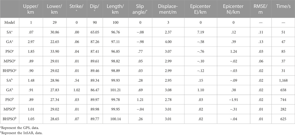
TABLE 1. Parameter settings of simulated strike-slip fault earthquake and inversion results of different methods.
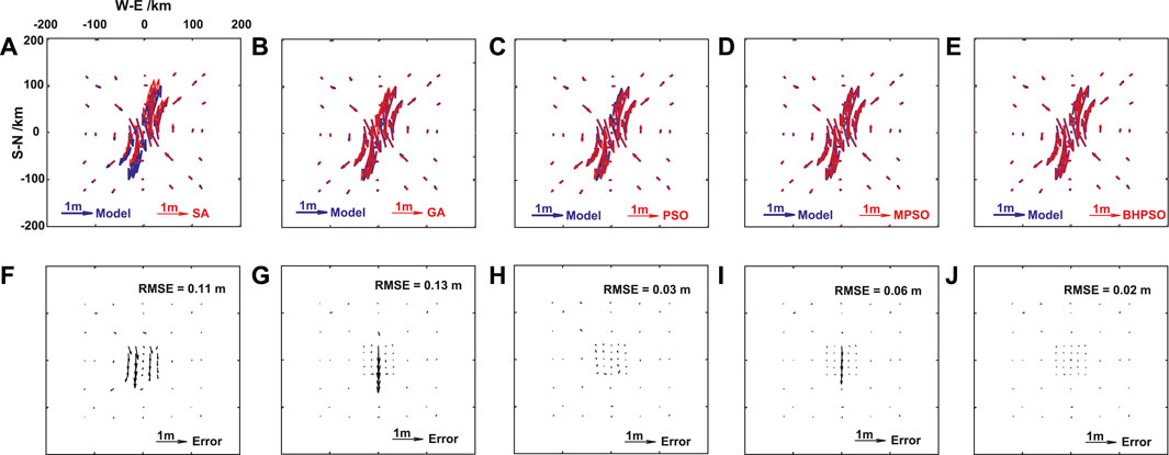
FIGURE 1. The comparisons of surface horizontal deformation (GPS data) of the Okada model results from the pure strike-slip fault earthquake by using fault parameters given by the model and inversed from five methods in Table 1. The surface horizontal deformation obtained by model and SA method (A), model and GA method (B), model and PSO method (C), model and MPSO method (D), and model and BHPSO method (E). The residual of surface horizontal deformation between the results of model and SA method (F), model and GA method (G), model and PSO method (H), model and MPSO method (I), model and BHPSO method (J). The blue arrows show the simulated surface horizontal deformation by the model in Table 1. The red arrows show the simulated surface horizontal deformation by using the fault parameters inversed from the five methods. The black arrows show the fitting residuals.
First, we used the Okada’s rectangular dislocation model and the parameters in Tables 1–3 to determine the static coseismic displacement field (Okada, 1985; Okada, 1992). We then added a normal distribution noise (errors) (mean = 0 and standard deviation = 1 cm) into the calculated coseismic displacement field and obtained the simulated GPS data. We calculated the LOS coseismic deformation field observed by InSAR (incident angle = 23° and azimuth angle = 105°), added a normal distribution noise (mean = 0 and standard deviation = 1 cm) into this coseismic deformation field, and obtained the simulated InSAR data. Finally, we used the above five methods and the simulated GPS and InSAR observation data for the fault parameter inversion. We calculated the corresponding fault parameters and RMSE of each method and wrote down the calcuation time of each fault parameter inversion (Tables 1–3; Figures 1–6). The computer used has Intel i5 (10th) CPU and 8 Gb RAM.
When we use the GPS data, the RMSEs of PSO and its improved algorithms (i.e., MPSO and BHPSO) are smaller than those of SA and GA for the pure strike-slip fault earthquake (Table 1). The major differences among the results of the five methods occur near the fault (black arrows in Figure 1), and their residual errors that occur along the strike are large (Figure 1). The residual errors of SA on both sides of the fault are big and consistent, and those on the fault trace line are small (Figure 1F). The residuals of GA are concentrated on the fault trace line and are considerably larger than those at other locations (Figure 1G). Based on the results in Table 1, we suggested that these differences stem from the large differences between the calculated average displacement and the true value on the fault.
Moreover, when we used the GPS data for the pure dip-slip fault earthquake, MPSO and BHPSO exhibit the best performance because they yield smallest RMSEs among the five methods (Table 2; Figure 2). For the pure dip-slip fault earthquake, the RMSEs of SA and GA are smaller than those for the pure strike-slip fault earthquake (Tables 1; 2, Figure 1; 2). The differences in the results of the five methods are concentrated in the hanging wall of the fault, and the residual errors are opposite on either sides of the fault (Figures 2F–H). The results from SA exhibit some big residual errors (black arrow in Figure 2F) near the fault, and the errors in the hanging wall are considerably larger than those in the footwall. This is consistent with the observations around real dip-slip fault earthquakes, such as the 1999 Mw 7.6 chi-chi earthquake, wherein the coseismic displacement in the hanging wall was bigger than that in the footwall (Ji et al., 2003). Far away from the fault, the inversion results of GA are bad, and an abnormally big residual error is present in the southern section of the fault (Figure 2G). The residual errors of the GA method in the hanging wall and footwall have the same order of magnitude, which is different from that observed for SA (comparison of Figure 2G; Figure 2F).

TABLE 2. Parameter settings of simulated dip-slip fault earthquake and inversion results of different methods.
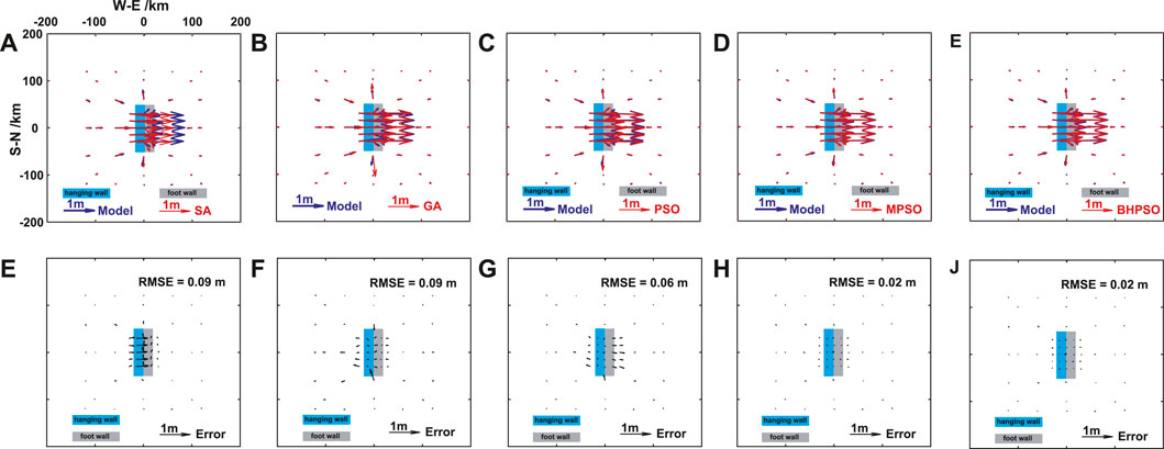
FIGURE 2. The comparisons of surface horizontal deformation (GPS data) of the Okada model results from the pure dip-slip fault earthquake by using fault parameters given by the model and inversed from five methods in Table 2. The surface horizontal deformation obtained by model and SA method (A), model and GA method (B), model and PSO method (C), model and MPSO method (D), and model and BHPSO method (E). The residual of surface horizontal deformation between the results of model and SA method (F), model and GA method (G), model and PSO method (H), model and MPSO method (I), model and BHPSO method (J). The blue arrows show the simulated surface horizontal deformation by the model in Table 2. The red arrows show the simulated surface horizontal deformation by using the fault parameters inversed from the five methods. The black arrows show the fitting residuals.
For the oblique-slip fault earthquake, when we use the GPS data, the MPSO and BHPSO exhibit the best performance among the five methods (Table 3; Figure 3). Moreover, SA, GA, and PSO exhibit relatively bad accuracy near the fault (black arrow in Figures 3F–H). SA affords an abnormally big residual error in the southern section of the fault (Figure 3F). The residual errors of GA gradually decrease from NE to SW (Figure 3G), showing bad inversion results on the northeastern part of the fault. The residual errors of PSO on the western side of the fault are bigger than those on the eastern side (Figure 3H). Table 3 signifies that these differences may be related to the difference between the inversed fault dip angle and the inversed fault slip angle.
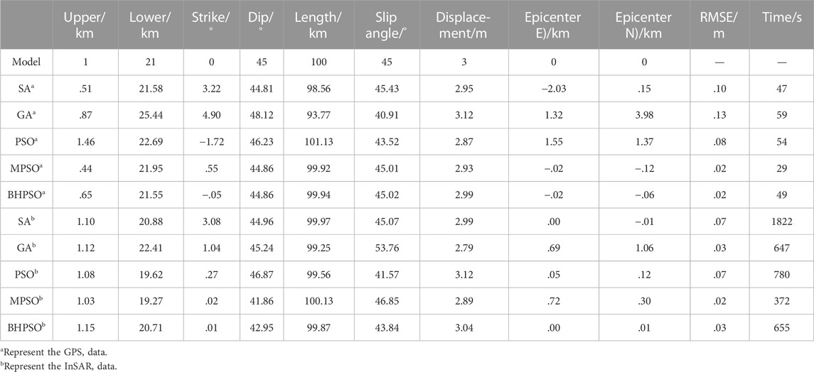
TABLE 3. Parameter settings of simulated oblique-slip fault and inversion results of different methods.
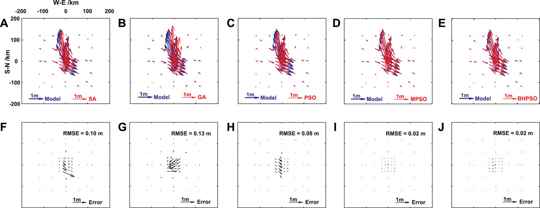
FIGURE 3. The comparisons of surface horizontal deformation (GPS data) of the Okada model results from the oblique-slip fault earthquake by using fault parameters given by the model and inversed from five methods in Table 3. The surface horizontal deformation obtained by model and SA method (A), model and GA method (B), model and PSO method (C), model and MPSO method (D), and model and BHPSO method (E). The residual of surface horizontal deformation between the results of model and SA method (F), model and GA method (G), model and PSO method (H), model and MPSO method (I), model and BHPSO method (J). The blue arrows show the simulated surface horizontal deformation by the model in Table 3. The red arrows show the simulated surface horizontal deformation by using the fault parameters inversed from the five methods. The black arrows show the fitting residuals.
For the pure strike-slip fault earthquake (using InSAR data), all the RMSEs of the five methods are small (Table 1; Figure 4). The MPSO and BHPSO have the lowest RMSEs, and perform best in these methods (Table 1; Figure 4). Hence, the results indicate that all the five methods are valid and accurate.
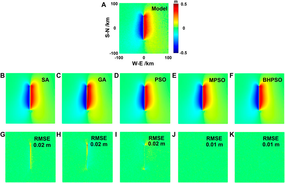
FIGURE 4. The comparisons of surface horizontal deformation (InSAR data) of the Okada model results from the pure strike-slip fault earthquake by using fault parameters given by the model and inversed from five methods in Table 1. The surface horizontal deformation obtained by model (A), SA method (B), GA method (C), PSO method (D), MPSO method (E), and BHPSO method (F). The residual of surface horizontal deformation between the results of model and SA method (G), model and GA method (H), model and PSO method (I), model and MPSO method (J), model and BHPSO method (K). The blue arrows show the simulated surface horizontal deformation by the model in Table 1. The red arrows show the simulated surface horizontal deformation by using the fault parameters inversed from the five methods. The black arrows show the fitting residuals. The positive value in color bar is the deformation away from the satellite, while the negative value is the deformation close to the satellite.
For the pure dip-slip fault earthquake (using InSAR data), the RMSEs of SA and GA methods are the same (Table 2), but the locations with the large residual errors in the two methods are different (Figure 5G; Figure 5H). The large residuals of SA are concentrated in the northern part of the fault, but those of GA occur along the whole fault (Figure 5). In this experiment, PSO and its improved algorithm (MPSO, BHPSO) have the relatively smaller RMSEs than SA and GA, and MPSO and BHPSO methods have the smallest RMSEs in these five methods (Table 2; Figure 5).
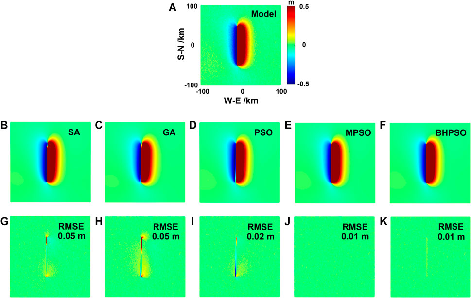
FIGURE 5. The comparisons of surface horizontal deformation (InSAR data) of the Okada model results from the pure dip-slip fault earthquake by using fault parameters given by the model and inversed from five methods in Table 2. The surface horizontal deformation obtained by model (A), SA method (B), GA method (C), PSO method (D), MPSO method (E), and BHPSO method (F). The residual of surface horizontal deformation between the results of model and SA method (G), model and GA method (H), model and PSO method (I), model and MPSO method (J), model and BHPSO method (K). The blue arrows show the simulated surface horizontal deformation by the model in Table 2. The red arrows show the simulated surface horizontal deformation by using the fault parameters inversed from the five methods. The black arrows show the fitting residuals. The positive value in color bar is the deformation away from the satellite, while the negative value is the deformation close to the satellite.
The RMSEs of both SA and PSO methods are larger than other threes methods (Table 3), for the oblique-slip fault earthquake inversion by using InSAR data. The RMSEs of GA, MPSO, and BHPSO are small, and hence they have high accuracy (Table 3 abd Figure 6). The distributions of residual errors of SA and GA are similar, and both show an opposite trend in the northern and southern parts of the fault. The residual errors of PSO method are consistent throughout the fault, and the directions of residual errors on different sides of the fault are opposite (Figure 6).
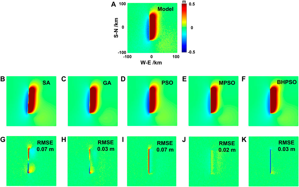
FIGURE 6. The comparisons of surface horizontal deformation (InSAR data) of the Okada model results from the oblique-slip fault earthquake by using fault parameters given by the model and inversed from five methods in Table 3. The surface horizontal deformation obtained by model (A), SA method (B), GA method (C), PSO method (D), MPSO method (E), and BHPSO method (F). The residual of surface horizontal deformation between the results of model and SA method (G), model and GA method (H), model and PSO method (I), model and MPSO method (J), model and BHPSO method (K). The blue arrows show the simulated surface horizontal deformation by the model in Table 3. The red arrows show the simulated surface horizontal deformation by using the fault parameters inversed from the five methods. The black arrows show the fitting residuals. The positive value in color bar is the deformation away from the satellite, while the negative value is the deformation close to the satellite.
For the three different types of earthquakes, generally, the calculation time of SA method is the longest, and that of GA and PSO is similar but less than that of SA; the calculation time of BHPSO is shorter than that of PSO; that of MPSO is the lowest (Tables 1–3). Therefore, SA has the lowest efficiency, the efficiency of GA and PSO is higher than that of SA, and BHPSO and MPSO exhibit the highest efficiency. The difference in the calculation times of these methods (Tables 1–3) stems from the number of control parameters and calculation principles of these algorithms. For example, SA has a wide search space and complex control parameters. Thus, it usually takes a long time to search and obtain the best parameters. In GA, the input parameters need to be encoded and the encoded data need to be mutated to simulate gene hybridization. This process is complex and it takes a relatively long time. BHPSO includes the black hole algorithm instead of the search radius in PSO, which can reduce the search time and improve the search efficiency. MPSO uses local particles to reduce the search space and search time.
In summary, for the inversion of the three different types of earthquakes using GPS or InSAR data, BHPSO and MPSO afford the lowest RMSEs and GA and SA afford the highest RMSEs. Furthermore, BHPSO and MPSO consume the least time, whereas GA and SA consume the most time. Hence, the accuracy of GA and SA is the lowest, and MPSO and BHPSO are the most accurate and effective. Additionally, the inversion results for the oblique-slip fault earthquake are generally bad (Figure 6) using the InSAR data, which may be related to the complex slip pattern on the fault (Figures 1–6).
On 15 May 2020, an Mw 6.5 earthquake occurred in the Monte Cristo Mountains of Nevada, United States of America. The epicenter location is at 117.850°W and 38.169°N and the source depth is 2.7 km (Table 4). Various studies have obtained the focal mechanism solution of this event (Hammond et al., 2020; Liu et al., 2021) (Table 4). We applied the above five inversion methods and the observed GPS data from Hammond et al. (Hammond et al., 2020) for the fault parameter inversion of this earthquake. First, we converted the latitude and longitude of the GPS data into local geodetic coordinates. We set the epicenter (117.850°W, 38.169°N) as the origin of the coordinates, transforming the longitudes and latitudes of the GPS stations into local coordinates (Figure 3). We used the five inversion methods to inverse the fault parameters of this earthquake from the transformed GPS data (Table 5).
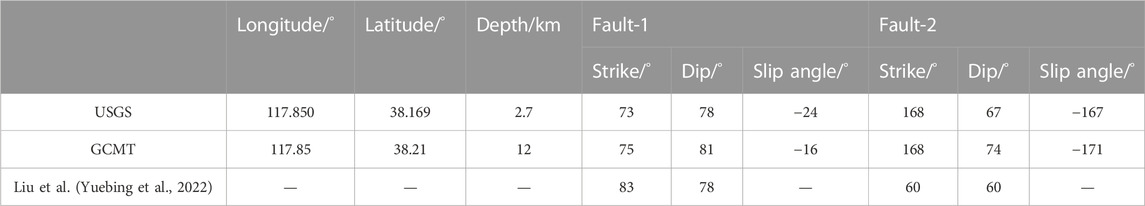
TABLE 4. Focal mechanism solution of the Nevada earthquake.
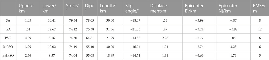
TABLE 5. The inversion results of fault parameters for the Nevada earthquake.
PSO and its improved algorithms performed better than SA and GA because PSO, MPSO, and BHPSO have smaller residual errors than SA and GA (Table 5). Comparison of the results of MPSO and BHPSO (Figure 7) shows that the residual error of MPSO was relatively large in the northwest of the epicenter (Figure 7B) but the distribution of the residual error from BHPSO was relatively uniform (Figure 7D), resulting in a high RMSE for MPSO and a low RMSE for BHPSO (Table 5). Among the five methods, BHPSO exhibited the best performance due to its smallest residual error (Table 5). Hence, the model results of BHPSO best fit the original GPS observation data (Figure 7; Table 5). Therefore, BHPSO is the most effective and accurate for single fault parameter inversion.
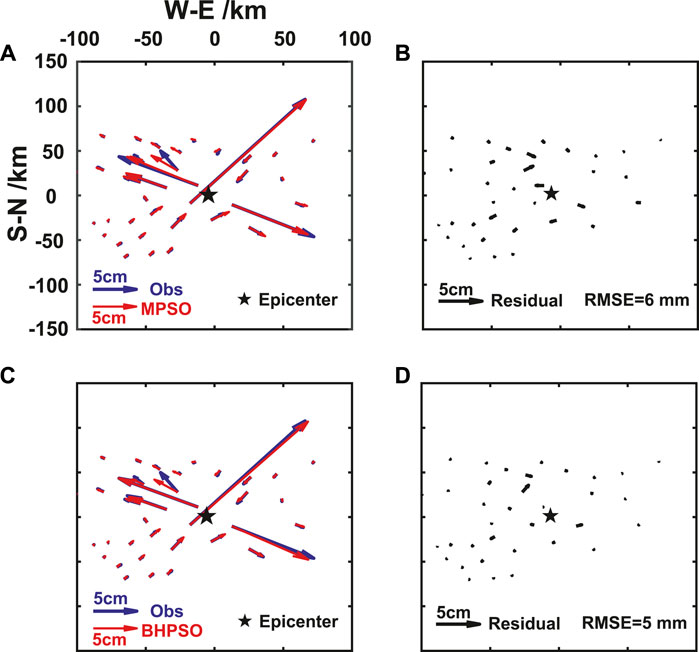
FIGURE 7. The comparisons of surface horizontal deformation (GPS data) of the observed and the Okada model results by using fault parameters given by the inversed from MPSO and BHPSO methods in Table 5. The surface horizontal deformation obtained by observed and MPSO method (A), observed and BHPSO method (C). The residual of surface horizontal deformation between the results of observed and MPSO method (B), observed and BHPSO method (D). Here, we only show the horizontal displacement and residuals because the vertical displacement is considerably smaller than the horizontal displacement. The blue arrow and its length represent the displacement from GPS data, the red arrow and its length represent the inversion results from MPSO or BHPSO. The black arrow and its length represent the residuals.
On 22 May 2021, a left-lateral strike-slip fault earthquake with Mw 7.4 occurred in Maduo County, Goluo Prefecture, Qinghai Province of China. The epicenter was located at 98.34°E and 34.59°N, and the source depth was ∼17 km from China Earthquake Networks Center (https://news.ceic.ac.cn). Many studies have investigated and inversed the parameters of the seismogenic fault and the earthquake rupture processes using the observed GPS, InSAR, and seismic wave data (Yuebing et al., 2022), (Hong et al., 2022), but they have obtained different fault parameter inversion results (Table 6).
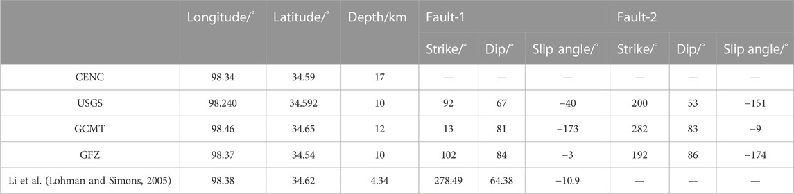
TABLE 6. Focal mechanism solution of the Maduo earthquake.
In this study, we used the abovementioned five inversions methods for the fault parameter inversion of this earthquake using the observed GPS (Yuebing et al., 2022) and InSAR data (Hong et al., 2022). Note that we did not use the joint inversion of multi-source data (joint inversion using the GPS and InSAR data), because this study aims to evaluate the accuracy and availability of the five inversion methods and not to find the optimal seismic fault parameters of the 2021 Mw 7.4 Maduo earthquake. We set the epicenter (98.34°E, 34.59°N) of this event as the origin and converted the longitudes and latitudes of the GPS and InSAR data into local plane coordinates. Additionally, we used equal weight inversion without considering the position information and the error ranges of the different observed data.
In the inversion study using GPS data, the strike angle obtained by SA was close to that obtained by a previous study ((Zhicai et al., 2021)), but it was very different from that obtained by the other four methods (nearly opposite slip along the fault strike on the fault) (Table 7). The dip angle obtained by SA was also much smaller than that obtained by the other four methods (Table 7) and that obtained in many previous studies ((Zhicai et al., 2021; Hong et al., 2022)). Hence, SA may be unsuitable for the fault parameter inversion of earthquakes of the type of the 2021 Maduo earthquake. The fault parameters obtained by GA and PSO were close to those obtained by MPSO and BHPSO, but the RMSEs of GA and PSO were relatively large (Table 7). Hence, the inversion results from GA and PSO did not well fit the GPS observation data. The inversion results of MPSO and BHPSO were consistent (Table 7; Figure 8), and they exhibited smaller residual errors than SA, GA, and PSO (Table 7). Among the five methods, MPSO and BHPSO afforded the best performance.
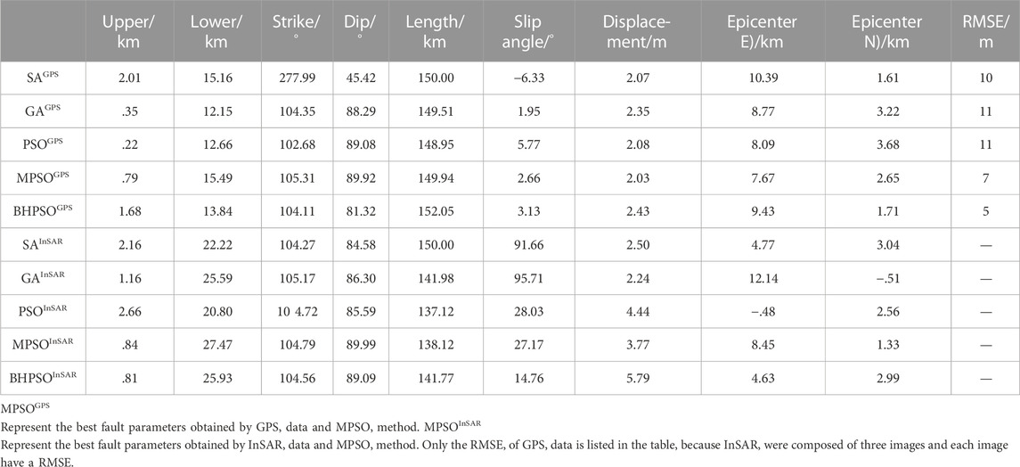
TABLE 7. The inversion results of fault parameters for the Maduo earthquake.
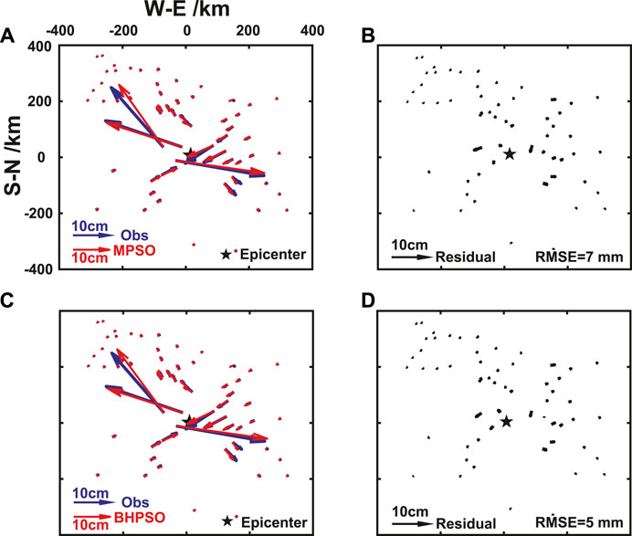
FIGURE 8. The comparisons of surface horizontal deformation (GPS data) of the observed and the Okada model results by using fault parameters given by the inversed from MPSO and BHPSO methods in Table 7. The surface horizontal deformation obtained by observed and MPSO method (A), observed and BHPSO method (C). The residual of surface horizontal deformation between the results of observed and MPSO method (B), observed and BHPSO method (D). The blue arrow and its length represent the displacement from GPS data, the red arrow and its length represent the inversion results from MPSO or BHPSO. The black arrow and its length represent the residuals.
In the inversion study using InSAR data, the results near the fault were poor (Figure 5). The residual errors of these methods were concentrated in the segments that have a complex fault slip pattern (Figure 9). Hence, when the observation data have good spatiotemporal resolution, the single fault model is unsuitable for fault parameter inversion because it cannot well fit the deformation details.
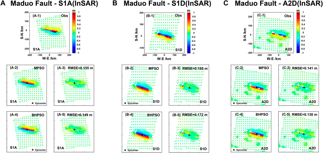
FIGURE 9. The comparisons of surface horizontal deformation (InSAR data) of the observed and the Okada model results by using fault parameters given by the inversed from MPSO and BHPSO methods in Table 7. (A) The Sentinel-1 ascending data and the inversion results from MPSO and BHPSO. (B) The Sentinel-1 descending data and the inversion results from MPSO and BHPSO. (C) The Sentinel-2 descending data and the inversion results from MPSO and BHPSO.
In the simulation experiments, for all three types of earthquakes (pure strike-slip, pure dip-slip, and oblique-slip fault earthquakes), the results of the fault parameter inversion using the simulated GPS data exhibited systematic differences from those using the simulated InSAR data. These differences could be related to the number of observation data. For example, the RMSEs obtained from the simulated GPS data were larger than those obtained from the simulated InSAR data. However, this does not denote that the results of inversion using the InSAR data are better than those using the GPS data. In fact, the residual errors between the model results and the data were large near the fault and small away from the fault due to the coseismic deformation magnitude at these locations.
Furthermore, the number of the simulated InSAR observation points was much larger than the number of simulated GPS stations, but most of the simulated InSAR points were distributed far away from the fault. When calculating the RMSEs (the average value of fitting errors between the model results and data at all observation points), the RMSEs from the simulated InSAR data should be lower than those from the simulated GPS data. Thus, herein, we simply compared the inversion results from the same type data such as either those from GPS data or those from InSAR data, and we did not compare the results inversed from these two types of data. SA and GA afforded the worst inversion results because the SA, GA, and PSO used herein are basic and not optimized. As shown in Tables 1–3, the RMSEs of SA, GA, and PSO were similar, signifying that they have similar effectiveness. MPSO and BHPSO are optimized versions of PSO. Hence, they afford smaller RMSEs than PSO and have higher efficiency and accuracy than PSO. Therefore, MPSO and BHPSO exhibited better performances than SA, GA, and PSO. This does not mean that the basic SA, GA and PSO are not suitable for fault parameter inversion. In this paper, we can conclude that the accuracy of fault parameters obtained by MPSO and BHPSO methods are better than that obtained by SA, GA and PSO methods. The inversion of fault parameter is a complex non-linear problem. Even the MPSO and BHPSO methods do not yield the most accurate seismic fault parameters. The advantages and disadvantages of these five methods are related to the standard of precision. If we only need to get the preliminary fault parameters, these five methods can be used.
Studies applying real observed InSAR data for seismic fault parameter inversion usually conduct down sampling (Lohman and Simons, 2005), which yields dense observation points near the fault and sparse observation points far away from the fault, similar to the distribution pattern of the GPS observation points (or GPS stations). In this study, we did not perform down sampling during the simulated InSAR data inversion but used it in the real observed InSAR data inversion (fault parameter inversion for the 2020 Mw 6.5 Nevada earthquake and 2021 M 7.4 Maduo earthquake). For our examples of the fault parameter inversion of real earthquakes, the accuracy and usability of the five methods considerably differed from the fault parameter inversion of the simulated earthquakes. This is because the observed data near the real fault zone contain numerous measurement errors, such as ionospheric disturbances, surface plants, water, and clouds, and the data quality varies with the locations and examples. In summary, we determined that MPSO and BHPSO usually perform better than the other three methods.
The differences among the inversion results of the five methods using real GPS data were less than those using real InSAR data. The real fault plane geometry and its coseismic rupture are complex—comprising bends, bifurcations, and multiple-fault rupture. GPS data cannot well comprehend the details of these fault geometries and ruptures, but the InSAR data can. Hence, in a single fault parameter inversion model using the InSAR data, large residual errors can occur at these complex locations. This results in larger residual errors in the InSAR data inversion than those in the GPS data inversion.
We used the simulated deformation data and real observed GPS and InSAR data to evaluate accuracy and availability of five geophysical inversion methods (SA, GA, PSO, MPSO, and BHPSO) for fault parameter inversion of different-type fault earthquakes. We drew our conclusions as below.
1) During seismic fault parameter inversion, the availability and accuracy of SA, GA, PSO, MPSO, and BHPSO are quite different.
2) We demonstrated that the new inversion method, BHPSO, can be used for seismic fault parameter inversion, and it has high accuracy in fault parameter inversion.
3) For fault parameter inversion of different-type fault earthquakes, MPSO and BHPSO perform better than the SA, GA, and PSO, due to their stable results and small residual errors. Particularly, in the fault parameter inversion of the oblique-slip fault earthquake, the inversion results of MPSO and BHPSO are significantly better than those of SA, GA, and PSO.
The data analyzed in this study is subject to the following licenses/restrictions: some data come from the references. Requests to access these datasets should be directed to xb_jin@whu.edu.cn.
XJ: Conceptualization, Methodology, Software, Data curation, Visualization, - Original draft, Investigation, Formal analysis. GL: Validation, Writing—Reviewing and Editing, Visualization, Funding acquisition. WZ: Writing—Original draft, Formal analysis.
This study is funded by the National Natural Science Foundation of China (41974107), and the National Key Research and Development Project of China (2021YFC3000605). The MATLAB software package we used to perform data fitting in this study can be found at https://www.mathworks.com/products/matlab.html?s_tid=hp_products_matlab.
The authors declare that the research was conducted in the absence of any commercial or financial relationships that could be construed as a potential conflict of interest.
All claims expressed in this article are solely those of the authors and do not necessarily represent those of their affiliated organizations, or those of the publisher, the editors and the reviewers. Any product that may be evaluated in this article, or claim that may be made by its manufacturer, is not guaranteed or endorsed by the publisher.
Caijun, X., and Yangmao, W. (2008). Nonho mogeneity of the crust from ms 7.9 manyi (tibet) earthquake with InSAR observation. Geomatics Inf. Sci. Wuhan Univ. 33 (8), 4.
De Natale, G., Crippa, B., Troise, C., and Pingue, F. (2011). Abruzzo, Italy, earthquakes of april 2009: Heterogeneous fault-slip models and stress transfer from accurate inversion of ENVISAT-InSAR data. Bull. Seismol. Soc. Am. 101, 2340–2354. doi:10.1785/0120100220
Díaz-Mojica, J., Cruz-Atienza, V. M., Madariaga, R., Singh, S. K., Tago, J., and Iglesias, A. (2014). Dynamic source inversion of the M6.5 intermediate-depth zumpango earthquake in central Mexico: A parallel genetic algorithm. J. Geophys. Res. Solid Earth 119, 7768–7785. doi:10.1002/2013jb010854
Dominguez, S., Avouac, J.-P., and Michel, R. (2003). Horizontal coseismic deformation of the 1999 Chi-Chi earthquake measured from SPOT satellite images: Implications for the seismic cycle along the Western foothills of central Taiwan. J. Geophys. Res. Solid Earth 108. doi:10.1029/2001jb000951
Hammond, W. C., Blewitt, G., Kreemer, C., Koehler, R. D., and Dee, S. (2020). Geodetic observation of seismic cycles before, during, and after the 2020 Monte Cristo range, Nevada earthquake. Seismol. Res. Lett. 92, 647–662. doi:10.1785/0220200338
Holland, H. J. (1975). Adaptation in natural and artificial systems. Ann Arbor, MI, USA: University of Michigan Press.
Hong, S., Liu, M., Liu, T., Dong, Y., Chen, L., Meng, G., et al. (2022). Fault source model and stress changes of the 2021 Mw 7.4 Maduo earthquake, China, constrained by InSAR and GPS measurements. Bull. Seismol. Soc. Am. 112, 1284–1296. doi:10.1785/0120210250
Ji, C., Helmberger, D. V., Wald, D. J., and Ma, K.-F. (2003). Slip history and dynamic implications of the 1999 Chi-Chi, Taiwan, earthquake. J. Geophys. Res. Solid Earth 108. doi:10.1029/2002jb001764
Jónsson, S. n., Zebker, H., Segall, P., and Amelung, F. (2002). fault slip distribution of the 1999 Mw 7.1 hector mine, California, earthquake, estimated from satellite radar and GPS measurements. Bull. Seismol. Soc. Am. 92, 1377–1389. doi:10.1785/0120000922
Kennedy, J. (1995). “Particle swarn optimization,” in Proceedings of the IEEE International Conference on Neural Networks, Perth, Australia, November 1995.
Kirkpatrick, S., Gelatt, C. D., and Vecchi, M. P. (1983). Optimization by simulated annealing. Science 220, 671–680. doi:10.1126/science.220.4598.671
Leyang, W., Xibo, J., Wenbin, X., and Guangyu, X. (2021). A black hole particle swarm optimization method for the source parameters inversion: Application to the 2015 calbuco eruption, Chile. J. Geodyn. 146, 101849. doi:10.1016/j.jog.2021.101849
Liu, C., Lay, T., Pollitz, F. F., Xu, J., and Xiong, X. (2021). Seismic and geodetic analysis of rupture characteristics of the 2020 Mw 6.5 Monte Cristo range, Nevada, earthquake. Bull. Seismol. Soc. Am. 111, 3226–3236. doi:10.1785/0120200327
Lohman, R. B., and Simons, M. (2005). Some thoughts on the use of InSAR data to constrain models of surface deformation: Noise structure and data downsampling. Geochem. Geophys. Geosystems 6. doi:10.1029/2004gc000841
Magen, Y., Ziv, A., Inbal, A., Baer, G., and Hollingsworth, J. (2020). Fault rerupture during the july 2019 ridgecrest earthquake pair from joint slip inversion of InSAR, optical imagery, and GPS. Bull. Seismol. Soc. Am. 110, 1627–1643. doi:10.1785/0120200024
Matsu'ura, M., Jackson, D. D., and Cheng, A. (1986). Dislocation model for aseismic crustal deformation at Hollister, California. J. Geophys. Res. Solid Earth 91, 12661–12674. doi:10.1029/jb091ib12p12661
McGinty, P., Darby, D., and Haines, J. (2001). Earthquake triggering in the Hawke's Bay, New Zealand, region from 1931 to 1934 as inferred from elastic dislocation and static stress modeling. J. Geophys. Res. Solid Earth 106, 26593–26604. doi:10.1029/2000jb000031
Metropolis, N., Rosenbluth, A. W., Rosenbluth, M. N., Teller, A. H., and Teller, E. (1953). Equation of state calculations by fast computing machines. J. Chem. Phys. 21, 1087–1092. doi:10.1063/1.1699114
Mirwald, A., Cruz-Atienza, V. M., Díaz-Mojica, J., Iglesias, A., Singh, S. K., Villafuerte, C., et al. (2019). The 19 september 2017 (Mw7.1) intermediate-depth Mexican earthquake: A slow and energetically inefficient deadly shock. Geophys. Res. Lett. 46, 2054–2064. doi:10.1029/2018gl080904
Nowroozi, A. A. (1985). Empirical relations between magnitudes and fault parameters for earthquakes in Iran. Bull. Seismol. Soc. Am. 75, 1327–1338.
Nunnari, G., Puglisi, G., and Guglielmino, F. (2005). Inversion of SAR data in active volcanic areas by optimization techniques. Nonlin. Process. Geophys 12, 863–870. doi:10.5194/npg-12-863-2005
Okada, Y. (1992). Internal deformation due to shear and tensile faults in a half-space. Bull. Seismol. Soc. Am. 82, 1018–1040. doi:10.1785/bssa0820021018
Okada, Y. (1985). Surface deformation due to shear and tensile faults in a half-space. Bull. Seismol. Soc. Am. 75, 1135–1154. doi:10.1785/bssa0750041135
Pedersen, R., Jónsson, S., Árnadóttir, T., Sigmundsson, F., and Feigl, K. L. (2003). Fault slip distribution of two June 2000 MW6.5 earthquakes in South Iceland estimated from joint inversion of InSAR and GPS measurements. Earth Planet. Sci. Lett. 213, 487–502. doi:10.1016/s0012-821x(03)00302-9
Shaorong, Z. (1991). Theory and application of dynamic geodetic inversion and physical interpretation. Wuhan, China: Wuhan university of surveying and mapping technology.
Stoffa, P. L., and Sen, M. K. (1991). Nonlinear multiparameter optimization using genetic algorithms; inversion of plane-wave seismograms. Geophysics 56, 1794–1810. doi:10.1190/1.1442992
Wanpeng, F., and Zhenhong, L. (2010). A novel hybrid PSO/simplex algorithm for determining earthquake source parameters using InSAR data. Prog. Geophys. 25 (4), 7.
Xueming, S., and Jiaying, W. (2008). Lecture on non-linear inverse methods in geophysics(4) Gentic Algorithm method. Chin. J. Eng. Geophys. 02, 129–140.
Xueming, S., and Jiaying, W. (2007). Simulated annealing method. Chin. J. Eng. Geophys. 03, 165–174.
Yuebing, W., Yu, L., Yi, C., Lianjiang, J., Hongbo, S., Zaisen, J., et al. (2022). Coseismic displacement and slip distribution of the 2021 May 22, Ms 7.4 Madoi earthquake derived from GNSS observations. Chin. J. Geophys. 65 (2), 14.
Zhang, L., Poulton, M. M., and Wang, T. (2002). Borehole electrical resistivity modeling using neural networks. GEOPHYSICS 67, 1790–1797. doi:10.1190/1.1527079
Keywords: fault parameter inversion, non-linear methods, MPSO, earthquake, maduo earthquake
Citation: Jin X, Luo G and Zhao W (2023) Accuracy evaluation on five non-linear methods for fault parameter inversion of different-type fault earthquakes. Front. Earth Sci. 10:1094623. doi: 10.3389/feart.2022.1094623
Received: 10 November 2022; Accepted: 30 December 2022;
Published: 17 January 2023.
Edited by:
Yanfei Wang, Institute of Geology and Geophysics (CAS), ChinaReviewed by:
Hua Gao, Jiangxi Normal University, ChinaCopyright © 2023 Jin, Luo and Zhao. This is an open-access article distributed under the terms of the Creative Commons Attribution License (CC BY). The use, distribution or reproduction in other forums is permitted, provided the original author(s) and the copyright owner(s) are credited and that the original publication in this journal is cited, in accordance with accepted academic practice. No use, distribution or reproduction is permitted which does not comply with these terms.
*Correspondence: Gang Luo, Z2x1b0BzZ2cud2h1LmVkdS5jbg==Z2FuZ2x1bzY2QGdtYWlsLmNvbQ==
Disclaimer: All claims expressed in this article are solely those of the authors and do not necessarily represent those of their affiliated organizations, or those of the publisher, the editors and the reviewers. Any product that may be evaluated in this article or claim that may be made by its manufacturer is not guaranteed or endorsed by the publisher.
Research integrity at Frontiers
Learn more about the work of our research integrity team to safeguard the quality of each article we publish.