 Yueyue Yu
 Xueting Yu
 Zhaoyong Guan
 Dingzhu Hu
 Chunhua Shi
 Dong Guo
 Jian Rao
- 1Key Laboratory of Meteorological Disaster, Ministry of Education (KLME), Joint International Research Laboratory of Climate and Environment Change (ILCEC), Collaborative Innovation Center on Forecast and Evaluation of Meteorological Disasters (CIC–FEMD), Institute for Climate and Application Research (ICAR), Nanjing University of Information Science and Technology, Nanjing, China
- 2LASG, Institute of Atmospheric Physics, CAS, Beijing, China
Stratospheric processes and their role in weather and climate have attracted increasing interests. The correspondence between the occurrence of pulse-like, stronger stratospheric poleward warm airmass transport (PULSE) events and the continental-scale cold air outbreak (CAO) events in northern hemispheric winter is found to be unstable from year to year. This increases the difficulties in utilizing the more predictable stratospheric variability in the sub-seasonal forecasts of CAOs, which can cause cold hazards. Using the ERA5 reanalysis data covering 37 winters (November–March) in the period 1979–2015, this study categorizes the CAO events over mid-latitudes of Eurasia (CAO_EA) and those over North America (CAO_NA) into two groups: those coupled with and those decoupled with the PULSE events. The coupled CAOs are further categorized into events that are, respectively, lead-coupled and lag-coupled with PULSEs. The intensity and affected area of extremely cold temperatures tend to be larger during CAOs that are coupled with PULSEs, particularly during the CAO_NA events that are lag-coupled with PULSEs and the CAO_EA events that are lead-coupled with PULSEs. Remarkable interannual and interdecadal variations are observed in the percentage of CAOs that are coupled with PULSEs for each winter, which is an important reference for determining the window of opportunity for skillful sub-seasonal forecasts of CAO by using the stratospheric signals. At both interdecadal and interannual timescales, a warm phase of the El Niño–Southern Oscillation (ENSO) in winter is favorable for the higher lag-coupling rate of CAO_NA and the lead-coupling rate of CAO_EA, and vice versa. The ENSO signals related to the interdecadal changes of the CAO coupling rate in winter can be traced back to the previous winter, while an ENSO phase transition from the previous winter to the current winter is closely related to the interannual changes of the CAO coupling rate.
1 Introduction
In recent years, with the support of the international scientific research program “Stratosphere–troposphere Processes and their Role in Climate” (SPARC), formulated by the World Climate Research Program (WCRP), an increasing number of new facts about the stratosphere–troposphere interaction have been revealed. The stratospheric polar vortex anomaly in winter has an important downward impact on the changes of tropospheric circulation and weather from 2 weeks to seasonal scale (Kodera et al., 1990; Kodera et al., 1991; Baldwin and Dunkerton, 1999; Wallace, 2000; Thompson et al., 2002; Kolstad et al., 2010; Wang and Chen, 2010; Cai et al., 2016; Kretschmer et al., 2018; Zhang et al., 2020).
The most famous weather impact from stratospheric variability is the relationship between the stratospheric polar vortex oscillation signals and cold air outbreak (CAO) events in the Northern Hemisphere, which are the most common extreme events in winter with potentially large impacts on human health, animals, agriculture, the energy industry, etc. In particular, weak stratospheric polar vortex anomalies or negative Northern Annular Mode (NAM) or stratospheric sudden warming (SSW) events are favorable to colder surface air temperatures or a higher occurrence of CAOs in mid-latitude regions of Eurasian and North American continents during the following months (Thompson et al., 2002; Kenyon and Hegerl, 2008; Tomassini et al., 2012; Kidston et al., 2015; Lehtonen and Karpechko, 2016; Garfinkel et al., 2017; Karpechko, 2018). Particularly, the cold anomalies tend to occur over North America (Eurasia) 1−2 weeks after (before) a weak stratospheric polar vortex event or a displacement-type SSW event, whereas cold anomalies tend to occur over both continents in 1 month around the split-type SSW events (Mitchell et al., 2013; Kidston et al., 2015; Lehtonen and Karpechko, 2016; Yu et al., 2018a; Choi et al., 2019; Choi et al., 2021).
In addition to the weaker-than-normal stratospheric polar vortex, recent studies (Iwasaki and Mochizuki, 2012; Iwasaki et al., 2014; Yu et al., 2014; Yu et al., 2015a; Yu et al., 2015b; Yu et al., 2015c; Cai et al., 2016; Liu and Chen, 2021) have noticed the weakening signals of the stratospheric polar vortex, namely, the wave-driven “pulse-like” strengthened poleward warm airmass transport into the polar stratosphere above 400 K (denoted as “PULSE”). This is also equivalent to an extreme planetary wave heat flux event (Shaw and Perlwitz, 2013; Shaw and Perlwitz, 2014). The PULSE events, via westward-tilted planetary waves of a deep structure, the enhanced poleward warm airmass transport into the polar stratosphere, or the stronger stratospheric warm branch of isentropic meridional mass circulation tends to be coupled with a stronger equatorward mass transport of cold airmass in the lower isentropic layers or a stronger cold branch of isentropic meridional mass circulation. Consequently, there is a close correspondence between the PULSE and the individual continental-scale CAOs (Cai et al., 2016; Yu et al., 2018a).
In addition, most operational models exhibit useful skills in predicting the stratospheric variability in extratropics at sub-seasonal timescales (Christiansen, 2005; Charlton and Polvani, 2007; Stan and Straus, 2009; Li and Ding, 2011; Zhang et al., 2013; Yoden et al., 2014; Tripathi et al., 2015; Cai et al., 2016; Yu and Ren, 2019; Rao et al., 2021; Scaife et al., 2022). Accordingly, the anomalous signals in the stratospheric polar vortex and related circulation become a potential predictability source for sub-seasonal to seasonal (S2S) forecasts of CAOs (Sigmond et al., 2013; Tripathi et al., 2015; Cai et al., 2016; Mariotti et al., 2018). Cai et al. (2016) constructed a hybrid paradigm by utilizing the useful prediction skills of operational models for PULSE events for predicting the timing of the occurrence of individual CAOs up to 1 month in advance. The stratosphere–troposphere coupling enhances the sub-seasonal predictability of northern Eurasian cold spells (Statnaia et al., 2022).
However, not all stratospheric signals can propagate down to the troposphere and effectively affect the occurrence of CAOs (Baldwin and Dunkerton, 2001; Black and McDaniel, 2004; Nakagawa and Yamazaki, 2006; Karpechko et al., 2017; Waugh et al., 2017; Zhang et al., 2019). In addition, though the experimental forecasts issued since 2014/2015 winter using the paradigm reported in Cai et al. (2016) yield an overall useful forecast skill for CAOs, particularly for those over mid-latitude regions of North America, the correspondence or coupling relationship between the occurrence of the PULSE and that of CAO is not stable from year to year. Only when the PULSE and CAO events are closely linked in winter, the window of opportunity for skillful sub-seasonal forecasts of CAO by using the stratospheric signals is open.
Therefore, three scientific questions are urgently needed to be addressed: i) what are the features of CAO events that are coupled and decoupled with stratospheric PULSE events? ii) How has the coupling relationship between the PULSE and CAO varied in the past 36 winters? iii) What are the possible influencing factors? To answer these questions, this study focuses on the CAO events, respectively, over mid-latitude Eurasian and North American continents during 37 winters (November–March) from 1979 to 2015, investigates the spatial patterns of surface air temperature (SAT) anomalies as well as the temporal variations of tropospheric and stratospheric circulation anomalies related to CAOs coupled/decoupled with stratospheric PULSE events, presents the interannual and interdecadal variations of the CAO–PULSE coupling rate, and finally discusses the possible impact from various sea surface temperature (SST) boundary forcing with significant interannual and interdecadal variabilities.
2 Data and methods
2.1 Data
The data used in this study include daily mean SAT, SST, and three-dimensional air temperature, geopotential height, meridional wind, and zonal wind fields derived from the 6-hourly ERA5 reanalysis data [Copernicus Climate Change Service (C3S)] (Hersbach et al., 2020) from January 1979 to December 2016. The data fields are on 0.5 latitude × 0.5 longitude grids and 37 pressure levels from 1,000 to 1 hPa. The daily anomaly field is obtained by removing the climatological mean annual cycle from the raw data. The monthly mean SST indices including the Pacific Decadal Oscillation (PDO), tropical Northern Atlantic (TNA) index, extreme eastern tropical Pacific SST index (Nino 1+2), east central tropical Pacific SST index (Nino 3.4), central tropical Pacific SST index (Nino 4), and Atlantic Multidecadal Oscillation (AMO) index are obtained from the NOAA CPC website (http://www.cpc.noaa.gov/). The North Pacific Gyre Oscillation (NPGO) index is downloaded from the website http://www.o3d.org/npgo/. Following the study by Saji et al. (1999), the Indian Ocean dipole (IOD) index is derived as the SST anomaly difference between the western (10°S–10°N, 50°–70°E) and eastern (10°S–0°, 90°–110°E) tropical Indian Ocean. The Indian Ocean Basin (IOB) index is derived as the average SST anomaly over the tropical Indian Ocean (40°−110 °E, 20°S−20 °N). Winter means in each year are obtained by averaging over the period from November of the current year to March of the next year. The climatological daily field was obtained by taking the average over the past 37 years for each calendar day from November 1 to March 31 and applying a 31-day running mean. Daily anomaly fields were obtained by removing the annual cycle.
2.2 Isentropic meridional mass fluxes and definition of PULSE events
The daily zonally integrated meridional mass fluxes in various isentropic layers are calculated using the same methods as in the studies by Pauluis et al. (2008), and Yu et al. (2015a), Yu et al. (2015b), and Yu et al. (2015c). The predefined 16 isentropic layers include the bottom layer below 260 K, 14 layers between adjacent isentropic levels (i.e.,
Following studies by Cai et al. (2016), and Yu et al. (2015a), Yu et al. (2015b), and Yu et al. (2018b), the vertical sum of the zonally integrated meridional mass fluxes at 60°N above 400 K is used to measure the meridional mass transport into the polar stratosphere, which is denoted as the ST60N index. Larger (smaller) values of ST60N indicate more (less) warm airmass transport into the polar stratosphere, which always warm and weaken (cool and strengthen) the stratospheric polar vortex. The period when the ST60N index continuously exceeds its 70th percentile (i.e., 1.53 × 10⁹ kg s−1) is selected and defined as an anomalously strong stratospheric mass circulation event or stratospheric polar vortex weakening event. For easy reference, such a stratospheric event is referred to as a PULSE event, following the study by Cai et al. (2016).
2.3 Definition of CAO events
Following studies by Cai (2003), and Yu et al. (2015a), Yu et al. (2015b), Yu et al. (2015c), Yu et al. (2018b), and Yu et al. (2018c), we first calculate the SAT anomalies. Then the winter means are removed from the anomaly fields in each winter to exclude interannual and longer timescale variabilities. The cold area index is defined as the percentage area of the SAT anomaly less than −0.5 local standard deviation in the mid-latitude region of North America (30°–60°N, 60°W–120°W) and mid-latitude Eurasia (30°–60°N, 0°–135°E), denoted as the CNA and CEA indices, respectively. A CAO_NA (CAO_EA) event is defined as a period when the CNA (CEA) index continuously exceeds its 70th percentile, which is 40% (36%). One CAO event can have several peaks, namely, several rounds of short-lived cold surges that take place during that cold period. By such definition, there are no significant interannual changes in the occurrence frequency of CAO events.
2.4 PULSE–CAO coupling index
The peak-weighted correspondence calculating method in the study by Yu et al. (2018b) is used to obtain the rate of CAO events accompanying PULSE events in each winter. The first step is to pair the peak of CAO in each winter with the closest peak of PULSE events and leave the other CAO peaks unpaired. For each winter, we define a variable Y as a function of the event number of CAO events, n, and peak number, k (k = 1, K(n)), where K(n) is the total number of peaks for the CAO event n, and the lag days of the CAO peak relative to the paired PULSE peak tlag. Y is set to 1 if the peak of the CAO is uniquely paired with a peak of the PULSE event; otherwise, Y is set to 0. The rate of CAO accompanying PULSE events as a function of tlag is calculated according to the following equation:
where wgt is a weighting function derived as follows:
Herein, C corresponds to either CNA or CEA, Cpeak (k, n) denotes the peak value of the cold area index (i.e., CNA or CEA) for the peak k of CAO event n, and C70th is the 70th percentile of the specific cold area index. If the CAO event n is single-peaked, that is, if K(n) = 1, then “wgt” is equal to 1. If the CAO event n is multi-peaked, that is, if K(n) > 1, then wgt is larger for the peak with larger amplitude. Thus, the correspondence between a PULSE event peak and a CAO event peak with larger amplitude will be given higher weight in counting the R. By definition, if all the peaks of CAO events over the mid-latitudes of the Eurasian or North American continents correspond uniquely to the peak of a PULSE event, then the sum of R at all time lags is equal to 1 or 100%.
A set of coupling indices is defined. The CAO_NAs that are coupled with PULSEs is defined as events that have one-to-one correspondence to PULSE events and occurred during the 2-week period centered at the peak of the corresponding PULSE event. The rate of CAO_NAs that are coupled with PULSEs in each winter is derived as the sum of R from tlag=−7 to tlag=7, denoted as the PULSE–CAO_NA coupling index. We further divide the CAOs that are coupled with PULSEs into lead- and lag-coupled groups. The rate of CAO_NAs that are lead-coupled with PULSEs is measured by the sum of R from tlag=−7 to tlag=−1, denoted as the PULSE–CAO_NAlead coupling index. Also, the rate of CAO_NAs that are lag-coupled with PULSEs is measured by the sum of R from tlag=0 to tlag=7, denoted as the PULSE–CAO_NAlag coupling index. If the CAO_NA was not paired with any PULSE event or it occur beyond the period from 7 days before to 7 days after the peak of PULSE events, it is referred to as a CAO_NA event decoupled with PULSEs. In the same fashion, coupling indices for CAO_EA are also derived and denoted as PULSE–CAO_EA, PULSE–CAO_EAlead, and PULSE–CAO_EAlag coupling indices.
2.5 Temporal decomposition
To extract the interannual variability of coupling indices and SST indices in winter, we used the ensemble empirical mode decomposition (EEMD; Huang et al., 1998; Huang et al., 1999; Wu and Huang, 2009) method. EEMD is quite versatile in a broad range of applications for extracting signals from data generated in noisy nonlinear and non-stationary processes (Huang and Wu, 2008; Ji et al., 2014). We first decompose the time series of a given index into intrinsic mode functions (IMFs). Then, we divide the IMFs into two groups based on the dominant frequency of each IMF according to the power spectrum obtained by the Fourier transform analysis. One group contains the IMFs with a dominant period shorter than 10 years, the sum of which is considered the interannual component. Also, the sum of the remaining IMFs is considered a component at interdecadal and longer timescales.
3 Spatial features of CAO events coupled/decoupled with PULSE
3.1 CAOs that occurred in mid-latitude North America
During all CAO_NA events (Figure 1A), the composite SAT anomalies are characterized by a zonally dipole pattern in the North American sector. Specifically, there are significant negative SAT anomalies over Canada and the northern United States, with the strongest cooling in Canada up to 6°C. In the meantime, the Bering Strait and Alaska are occupied by warm anomalies. Such features can be observed in both CAO_NA events that are coupled and decoupled with PULSEs (Figures 1B,C). However, the magnitudes of the warm SAT anomalies are slightly larger, and the cold SAT anomalies over the North American continent invade more southward when the CAO_NAs are coupled with PULSE events (contours in Figure 1C). Among the CAO_NA events that are coupled with PULSEs, the zonally dipole pattern of SAT anomalies is more significant during the CAO_NA events that occurred in the week following the peak dates of PULSE events (Figure 1E), while the CAO_NA events that occur in the week before PULSE events are characterized by cold SAT anomalies mainly in the central-eastern half of the North American continent (Figure 1D). The difference in composite SAT anomalies between these two types of PULSE-coupled CAO_NA events can be seen more clearly from the contours in Figure 1E.
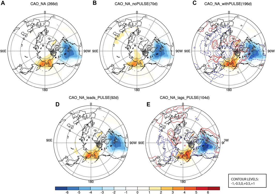
FIGURE 1. Composite mean maps of surface air temperature (SAT) anomalies during CAO_NA events in winters (November–March) from 1979 to 2015. (A) All CAOs; CAOs that are (B) decoupled from and (C) coupled with stratospheric PULSE events; and CAOs that are coupled with PULSEs and occurred within the week, respectively, (D) before and (E) after the peak dates of PULSEs. Only the composites above the 95% confidence level using two-sided Student’s t test are shown. Contours in panel (C) denote the SAT anomaly difference between (C,B), and contours in panel (E) denote the SAT anomaly difference between (E,D).
We further examine the possible dependence of the occurrence of extreme cold temperatures during CAO_NA events on the coupling or decoupling relationship with stratospheric PULSE events. Displayed in Figure 2 are the probability maps for the occurrence of SAT below normal by at least 1 LSD during all CAO_NA events and events belonging to different coupling groups. During all CAO_NA events, extreme cold temperatures occur most frequently over the eastern North America with occurrence probabilities higher than 45% (Figure 2A). Figures 2B,C show that both the CAO_NAs coupled and decoupled with PULSEs exhibit similar features, but the occurrence probabilities of extreme cold temperatures in the central and southeast United States are 5–10% higher during the CAO_NA events that are coupled with PULSE events than those decoupled CAO_NA events. Among the CAO_NA events that are coupled with PULSE events (Figures 2D,E), those that occur within 1 week after the peak dates of PULSE events are more likely to have extreme cold temperatures in the western half of the North American continent including the west coast and central United States and western Canada, where the climate is typically mild; thus, cold extremes may cause more threat to the energy industry and health risk (Cellitti et al., 2006; Palmer, 2014; Cohen et al., 2018). CAO events that occur within the week before the PULSE events are more likely to have extreme cold temperatures in the eastern areas.
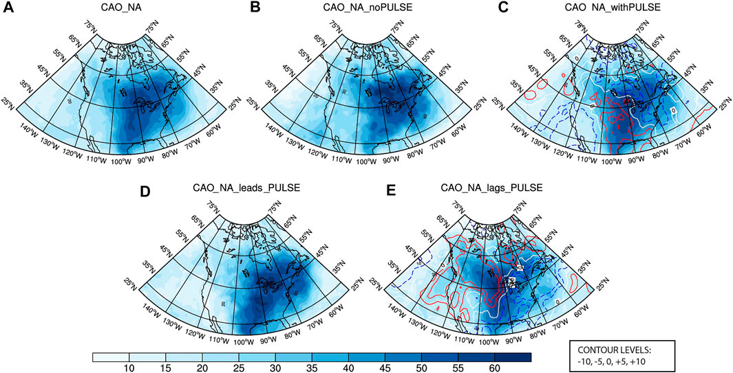
FIGURE 2. Similar to Figure 1 but for the occurrence probability of SAT anomalies <−1 LSD during CAO_NA events in the North American sector.
3.2 CAOs that occurred in mid-latitude Eurasia
The composite SAT anomalies during all CAO_EA events are characterized by a meridional dipole pattern (Figure 3A), namely, significant cold SAT anomalies in the mid-latitudes but warm anomalies in the high latitudes. This SAT anomaly pattern related to CAO_EA is consistent with that in many previous studies (Cohen et al., 2014; Ma and Zhu, 2020; Zhang et al., 2021). Maximum cold temperature anomalies are found in the northeast Asia and the Eastern European Plain, which are up to −4°C. Such features can be observed in mainly the CAO_EA events coupled with PULSEs (Figure 3B), and the magnitudes of both the cold anomalies over the Eurasian continent and the warm anomalies in the high latitudes are larger (contours in Figure 3C). While in those events decoupled with PULSEs (Figure 3C), the warm anomalies rarely occur in the higher latitudes but occur in the western Pacific instead. Among the CAOs that are coupled with PULSE events, the cooling intensity in Asia is much stronger during the CAOs that occur in the week before the peak dates of PULSEs, while the magnitudes of cold SAT anomalies in Western Europe are much larger during the CAOs that occur in the week after the peak dates of PULSEs (Figures 3D,E).
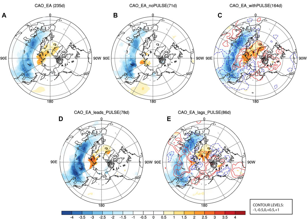
FIGURE 3. As in Figure 1, but for CAOs that occurred in Eurasia.
Probability maps for the occurrence of SAT anomalies below −1 LSD during CAO_EA events (Figure 4A) further show that during all the CAO_EA events, the regions with the largest probability of extreme cold temperatures are mid-latitude East Asia (25°N–60°N, 100°E–150°E), followed by Europe (35°N–55°N, 0°–60°E). Also, this feature can be observed in both CAO events coupled and decoupled with PULSE events (Figures 4B,C). However, during the CAO_EAs that are coupled with PULSEs, the probabilities of extreme cold temperatures are much larger in most regions of mid-latitude Eurasia, particularly in East Asian and European longitudinal bands, than in those during the CAOs that are decoupled with PULSEs. During the coupled CAOs that occur 1 week before PULSEs, the probabilities of extreme cold temperatures are higher in central and East Asia except on the east coast than in those during the coupled CAOs that occur 1 week after PULSEs. This indicates that stronger, continental-scale CAOs tend to occur before the PULSE event or a weakening of the stratospheric polar vortex. This is somewhat consistent with the Eurasian SAT anomalies that are often found before a negative NAM event or a displacement-type SSW event (Kolstad et al., 2010; Lehtonen and Karpechko, 2016; Yu et al., 2022). Western Europe, Japan, and Korea, however, are more likely to experience a higher probability of extreme cold temperatures when the CAOs occur within the week after PULSEs. The cold extremes across Europe and East Asia have been reported to relate to the negative phase of the Arctic Oscillation/North Atlantic Oscillation, which tends to follow a weaker stratospheric polar vortex due to the stratospheric downward impact (Hurrell, 1995; Thompson and Wallace, 1998; Jeong and Ho, 2005; Cattiaux et al., 2010; Lü et al., 2020).
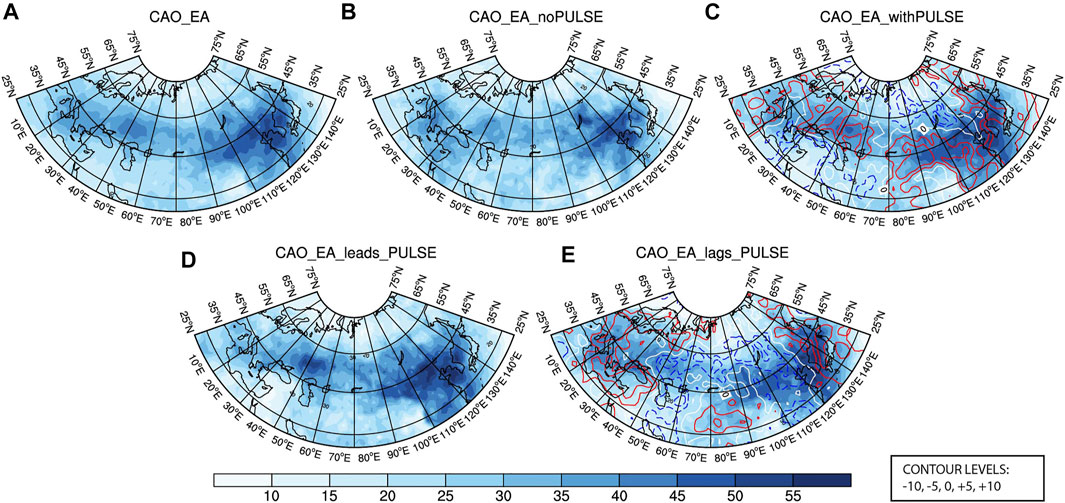
FIGURE 4. As in Figure 2, but for CAOs that occurred in Eurasia.
To sum up, we found several features distinct between CAOs that are coupled and decoupled with stratospheric PULSEs. For CAO_NA events, extreme cold temperatures tend to occur in the central and southeast United States when coupled with PULSEs. When CAO_NA events are lag-coupled with PULSEs, the cold anomalies tend to be stronger and spread more southward, and extreme cold temperatures are more likely to occur in the west coast and the central United States, and in western Canada. When CAO_NA events were lead-coupled, the eastern areas of the North American continent were more likely to have extreme cold temperatures. For CAO_EA events, extreme cold anomalies tend to be significantly stronger when coupled with PULSEs, especially those that are lead-coupled with PULSEs. More frequent extreme cold temperatures occur in Western Europe, Japan, and Korea when CAO_EA events are lag-coupled, while extreme cold temperatures tend to occur in the central regions of Eurasia when CAO_EA events are lead-coupled.
4 Tropospheric and stratospheric circulation anomalies associated with CAOs coupled/decoupled with PULSEs
4.1 Isentropic meridional mass circulation at 60°N
The lead-lag evolutions of the zonally integrated meridional mass flux anomalies at 60°N at various isentropic layers during CAO_NA and CAO_EA events (Figure 5) confirm the stratosphere–troposphere coupling/decoupling situation for each group of CAO events. We can see an anomalously strong stratospheric poleward warm air branch linked to PULSE-coupled CAO_NA and CAO_EA events, indicated by the significantly positive values of meridional mass flux anomalies in the stratospheric layers above 315 K around the peak dates of CAOs (Figures 5C,H). In contrast, the stratospheric meridional mass flux anomalies are generally negative or close to zero during the 2 weeks around the peak dates of CAOs that are decoupled with PULSEs (Figures 5B,G). In the troposphere, during the CAO events that are coupled with PULSEs, zonally integrated meridional mass flux anomalies tend to be significantly negative in layers below 280 K but positive in isentropic layers between 280 K and 315 K during the period of 3–4 days before the peak time of CAOs, as shown in Figures 5C,H. This indicates that the stronger equatorward cold branch together with the poleward warm branch results in continental-scale CAO events, confirming previous studies (Yu et al., 2015a; Yu et al., 2015b; Yu et al., 2015c). During CAOs that are decoupled with PULSEs (Figures 5B,G), however, the strengthening of cold and warm branches in the troposphere before peak dates of CAOs is not statistically significant, which implies that there are no robust global-scale atmospheric circulation anomalies related to these groups of CAOs.
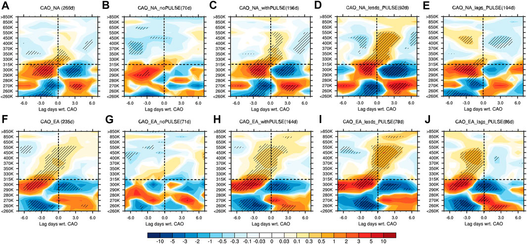
FIGURE 5. Meridional mass flux anomalies for latitudinal integration at 60°N at various isentropic layers at lag times from −7 to 7 days relative to the peak days of (A) all CAO_NA events, (B) CAO_NAs that are decoupled with PULSE events, (C) CAO_NAs that are coupled with PULSE events, (D) CAO_NAs that are lead-coupled with PULSEs, and (E) CAO_NAs that are lag-coupled with PULSEs. (F–J) are as (A–E) but for CAO_EA events. Slashed areas denote the composites statistically significant above the 95% confidence level using two-sided Student’s t test. The horizontal dashed line roughly marks the tropopause level, which is about 315 K.
The strengthening of the tropospheric cold and warm branches leads to the strengthening of the stratospheric poleward warm air branch by about 1 week associated with CAO events that occur before PULSEs (Figures 5D,I), whereas the strengthening of stratospheric and tropospheric branches is almost simultaneous during CAOs that occur after PULSE events (Figures 5E,J). Comparing the tropospheric cold and warm branches related to the CAO events that are, respectively, lead-coupled and lag-coupled with PULSEs, we see no significant difference in their intensity, but the anomalously strong tropospheric cold and warm branches tend to persist longer for CAO_EAs that occur before PULSE events and CAO_NAs that occur after PULSE events. The persistent stronger equatorward cold air branch may accumulatively strengthen the cold temperature anomalies, resulting in colder SAT anomalies as well as a higher occurrence probability of extremely cold temperatures during CAO_EA events that occur within 1 week before PULSEs and colder SAT anomalies during CAO_NA events that occur within 1 week after PULSEs.
Therefore, how the CAO is coupled with the stratospheric PULSE events highly depends on the coupling relationships between the tropospheric equatorward cold air branch and the stratospheric poleward warm air branch of isentropic meridional mass circulation across the polar circle.
4.2 Polar cap-averaged geopotential height (PCH)
The PCH fields are derived from the 60°−90°N areal mean geopotential height. PCH anomalies are next investigated to yield the variations in polar vortex intensity associated with CAO_NA and CAO_EA events that are coupled or decoupled with PULSEs (Figure 6A–C; Figure 6F–6H). One common feature that can be found between CAO events is the positive PCH anomalies at the tropospheric levels, which correspond to a weaker tropospheric polar vortex or a negative phase of AO (not shown). Such a weaker polar vortex has been reported to be one of the favorable large-scale circulation anomalies for the higher occurrence of CAOs over Eurasia or/and North America (Thompson and Wallace, 1998; Thompson and Wallace, 2001; Wettstein and Mearns, 2002; Cohen et al., 2010). However, we can see large contrast in the stratospheric polar vortex intensity between the CAO events that are coupled and decoupled with PULSEs. The PCH anomalies are persistently negative during the 1 month centered at the peak dates of CAOs that are decoupled with PULSEs, suggesting an anomalously strong state of the stratospheric polar vortex, while the weakening of polar vortex is confined within the troposphere. In contrast, significantly positive PCH anomalies can be seen associated with CAOs that are coupled with PULSEs, indicating a weaker stratospheric polar vortex accompanied by a weaker tropospheric polar vortex. This clearly reflects the existence of active troposphere–stratosphere interactions in this situation.
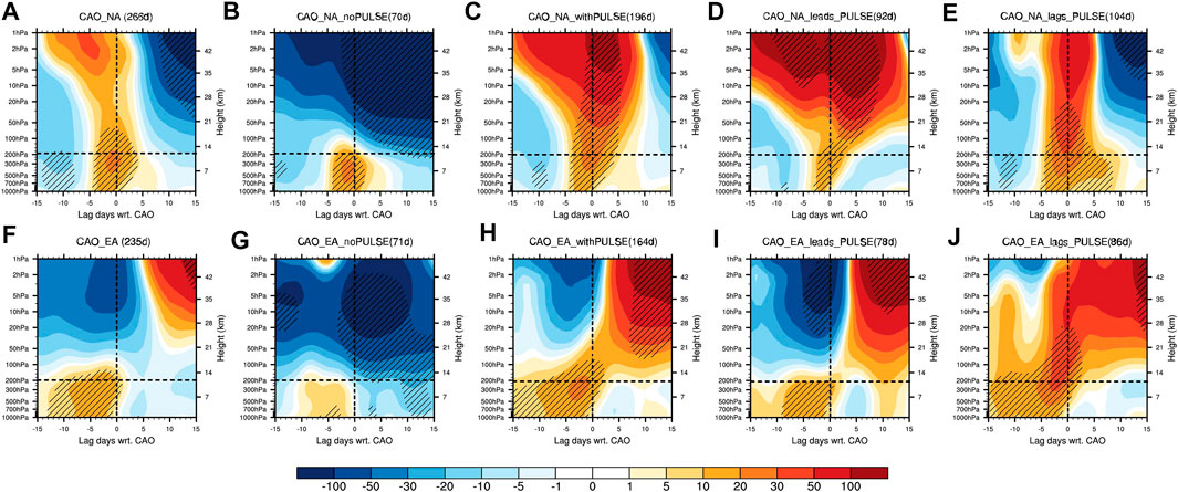
FIGURE 6. As in Figure 5, but for the geopotential height anomalies averaged over the polar cap (60°−90°N) at various isobaric levels. The horizontal dashed line roughly marks the tropopause level, which is 150–200 hPa.
The stratospheric polar vortex intensity exhibits different evolution features between CAO events that are lead-coupled and lag-coupled with PULSEs. During CAO_NA events that are lead-coupled with PULSEs (Figure 6D), the positive PCH anomalies have already been in the upper stratosphere above 10 hPa in the 2 weeks before peak dates of CAO_NA and showing an upward propagation from the lower troposphere at day −3 to the stratospheric levels at day +5. This suggests that for CAO_NA events that occur before PULSEs, the stratospheric polar vortex is already weakened, and the role of PULSE events driven by strengthened upward propagating waves related to the CAO_NA events acts to weaken the stratospheric polar vortex further. For the CAO_NA events that are lag-coupled with PULSEs (Figure 6E), the positive PCH anomalies are found at almost all levels in the week centered at the peak dates of CAO_NA, indicating a weakened polar vortex throughout the troposphere and lower-middle stratosphere. This weakened polar vortex is almost simultaneous with the stronger stratospheric poleward warm air branch and tropospheric equatorward cold air branch. It may reflect the situation when a very quick upward wave propagation process takes place, resulting in baroclinically instable waves of a deep structure in vertical. Such anomalous wave activities cause the almost simultaneous strengthening of tropospheric warm and cold branches and the stratospheric warm branch. During CAO_EA events that occur before PULSEs (Figure 6I), the PCH anomalies at stratospheric levels above 20 hPa are negative in the 2 weeks before peak dates of CAO_EA and reverse signs in the 2nd week after peaks. The timing of the sign reversal of PCH anomalies corresponds well to the stronger stratospheric warm branch in the period from day −1 to day +5, which lags the stronger tropospheric warm and cold branches. This suggests a significant weakening of the stratospheric polar vortex induced by PULSE events, whereas the PULSEs are driven by gradual upward propagated tropospheric waves related to CAO_EA events. This surpports previous studies showing that the enhanced upward planetary waves always originate from East Asia and effectively weaken the stratospheric polar vortex (Matsuno, 1971; Andrews et al., 1987; Polvani and Waugh, 2004). This is consistent with the common situation before an extremely weak stratospheric polar vortex event such as SSW. For the CAO_EA events occurring after PULSEs (Figure 6J), the simultaneously weakened polar vortex throughout the troposphere and lower-middle stratosphere is also observed, representing the almost simultaneous strengthening of tropospheric and stratospheric branches due to fast-propagating and deep-structure waves from the troposphere to the middle stratosphere.
Therefore, the CAO events that are coupled with PULSEs account for about 75% of the total CAOs occurred in mid-latitude regions of North America and Eurasia. These CAO events tend to have colder temperatures with a wider impact area, which is related to the coupling between the stratospheric poleward warm branch and the tropospheric equatorward cold branch of isentropic meridional mass circulation near the polar circle. The CAO_EA events that occur before PULSEs are always related to stronger planetary waves that can gradually propagate upward and thus correspond to the transition of the stratospheric polar vortex from a stronger-than-normal state to a weaker-than-normal state. The CAO_NA events that occur before PULSEs are always preceded by an already-weakened stratospheric polar vortex; thus, the related tropospheric waves propagate upward to further weaken the vortex. The CAO_NA and CAO_EA events that are lag-coupled with PULSEs are always attributed to the simultaneous strengthening of tropospheric poleward warm and equatorward cold branches and the stratospheric poleward warm branch of the isentropic meridional mass circulation, which are related to fast-propagating and deep-structure waves from the troposphere to the middle stratosphere.
5 Variations of coupling indices and possible impact from SST forcing
5.1 Temporal variations of coupling indices between PULSE and CAO
In addition to the fact that whether the CAO event is coupled with a PULSE or not can affect its intensity and impact area, the rate of CAO events that are coupled with stratospheric PULSEs for each winter is an important reference for using the stratospheric circulation signal to do sub-seasonal forecasts of CAOs. In this section, we examine the temporal evolution of coupling indices between PULSE and CAO events over mid-latitude North America and Eurasia, as shown in Figures 7, 8. It is seen that there are significant year-to-year variations in the coupling relationship between CAOs and PULSEs. For instance, the PULSE–CAO_NAlag coupling index was up to 80% in 2001 but close to 0% in 1983 and 2005. Only in winters with higher values of coupling indices, PULSE events can be used as a stratospheric predictor of CAOs, and the hybrid paradigm proposed by Cai et al. (2016) would be useful.
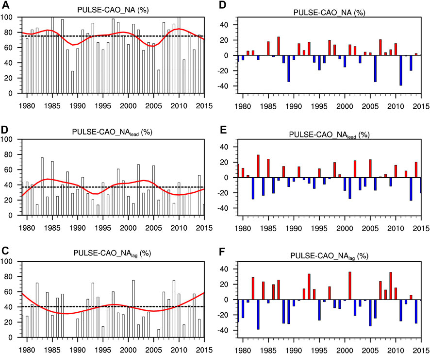
FIGURE 7. Time series of coupling indices (units: %) between PULSE and CAO_NA ((A) PULSE-CAO_NA, (B) PULSE-CAO_NAlead, and (C) PULSE-CAO_NAlag) from 1979 to 2015 in winters (November–March) (red lines: interdecadal components; the dotted lines: averages of interdecadal components). (D–F) As in (A–C) but for interannual components.
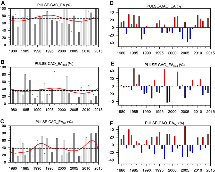
FIGURE 8. As in Figure 7, but for the coupling indices between CAO_EA and PULSE ((A), (D) PULSE-CAO_EA; (B), (E) PULSE-CAO_EAlead; and (C), (F) PULSE-CAO_EAlag).
We further decompose the PULSE–CAO coupling indices into interdecadal and interannual components. The coupling indices exhibit obvious interdecadal variations over a time period of about 15 years, and the variation range is about 20–30%. The variation range of the interannual component of the PULSE–CAO coupling indices is 30–40%, which is slightly larger than that of their interdecadal components. The PULSE–CAO_EAlag and PULSE–CAO_EAlead indices, in particular, have the largest interannual variations compared to the other coupling indices.
5.2 Correlation analyses between coupling indices and SST forcing indices
5.2.1 Simultaneous correlations
The following question still remains: what influences the variations of the PULSE–CAO coupling relationships from interannual to interdecadal timescales? We here explore the SST forcing from interannual to interdecadal timescales (including Nino, TNA, AMO, PDO, NPGO, IOB, and IOD) via examining their correlations with coupling indices.
As seen from Tables 1, 2, the correlations of the total and interannual components of the PULSE–CAO_NA and PULSE–CAO_EA coupling indices with all the selected SST-related indices are statistically insignificant. The correlations are mostly statistically insignificant at interdecadal timescales as well, except for the positive correlation between the interdecadal PULSE–CAO_NA coupling index and Indian Ocean SST signals (IOB and IOD) and the negative correlation between the interdecadal PULSE–CAO_EA coupling index and the NPGO index in current winter.
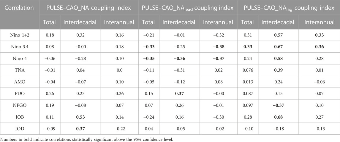
TABLE 1. Correlation coefficients of various SST-related indices with the PULSE–CAO_NA coupling indices and their interdecadal and interannual components in winters (November–March) from 1979 to 2015.
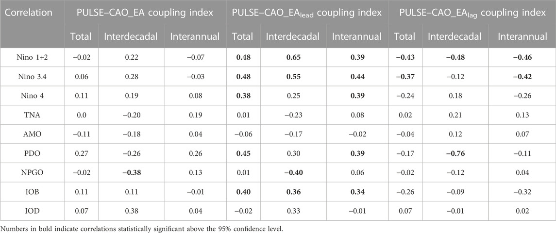
TABLE 2. As in Table 1, but for the PULSE–CAO_EA coupling indices.
After separating the lag-coupling and lead-coupling situations, the relationship of coupling indices with many SST forcing becomes robust. It is seen that among the Nino indices, the Nino 3.4 index has the largest significant positive correlations with the PULSE–CAO_NAlag and PULSE–CAO_EAlead indices at both interannual and interdecadal timescales. The Nino 4 (Nino 1+2) index has the largest negative correlation with the PULSE–CAO_NAlead (PULSE–CAO_EAlag) index. This indicates that not only the phase but also the type of ENSO plays an important role in influencing the PULSE–CAO coupling relationship. A warm phase of traditional ENSO tends to provide favorable boundary conditions for the coupling situation in which the CAO takes place in mid-latitude Eurasia first and then the stratospheric PULSE occurs. Following the PULSE, the CAO occurs in mid-latitude North America. Associated with the other coupling situations is a slightly westward or eastward shift of warming in the equatorial Pacific. In addition, the IOB mode that is modified by ENSO via the “atmospheric bridge” with a lag time of half a year (Alexander and Scott, 2002; Ashok et al., 2003) also shows significantly positive correlations with the PULSE–CAO_NAlag index at the interdecadal timescale and with the PULSE–CAO_EAlead index at both the interannual and interdecadal timescales. Since the correlations are not as large as Nino indices, we may expect that the relation of IOB with coupling indices may be attributed to the linkage between ENSO and IOB and ENSO’s impact on the coupling indices. The interdecadal PULSE–CAO_NAlag index also has positive correlations with TNA and negative correlations with NPGO, while the NPGO is also negatively correlated with the interdecadal PULSE–CAO_EAlead index. The interdecadal PULSE–CAO_EAlag index is related to the negative PDO, while the interannual PULSE-CAO_EAlead is related to the positive PDO. The relationship is further confirmed by the regression maps of NDJFM mean SST onto these coupling indices (Figures 9, 10).
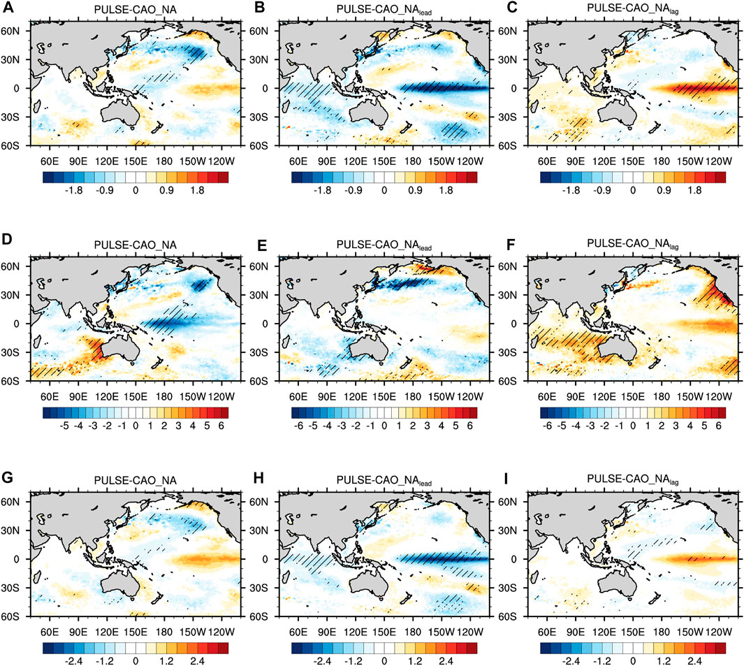
FIGURE 9. Regression maps of NDJFM mean SST anomalies during 1979–2015 against (A) the PULSE–CAO_NA index, (B) the PULSE–CAO_NAlead index, and (C) the PULSE-CAO_NAlag index. (D–F) and (G–I) are the same as (A–C) but for regressions against the interdecadal and interannual components of coupling indices, respectively. Slashed areas denote the regressions above the 95% confidence level using two-sided Student’s t test.
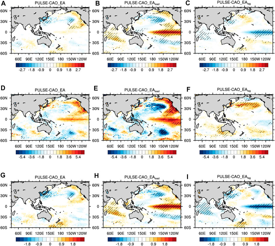
FIGURE 10. As in Figure 9, but for the PULSE–CAO_EA, PULSE–CAO_EAlead, and PULSE–CAO_EAlag coupling indices.
Therefore, most of the SST forcing in the tropical and subtropical Pacific has a robust impact on the PULSE–CAO coupling relationships. This impact is possibly through the stratosphere–troposphere coupling process, particularly planetary waves and their vertical propagation modified by Pacific SST anomalies as found by previous studies (García-Herrera et al., 2006; Manzini et al., 2006; Jadin et al., 2010; Hurwitz et al., 2012; Woo et al., 2015; Kren et al., 2016; Hu et al., 2018; Hu and Guan 2018; Hu et al., 2019).
5.2.2 Lead/lag correlations
In addition to the SST forcing in the current winter, the influence of SST forcing on the PULSE–CAO coupling indices can be traced back to the preceding seasons. Displayed in Figure 11 are the correlation coefficients between the interdecadal and interannual components of the PULSE–CAO lead-/lag-coupling indices in the winter and the SST indices from September of the previous year to May of the next year.
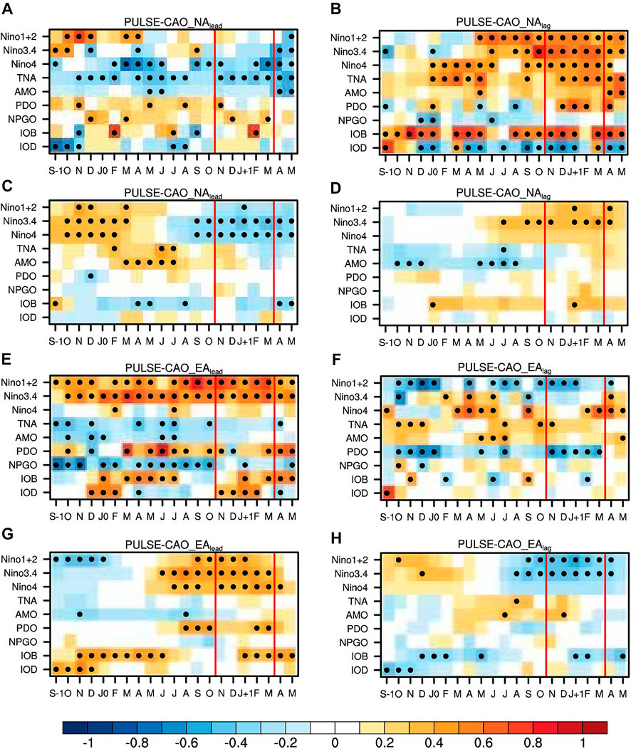
FIGURE 11. Correlation coefficients between monthly SST indices from September of the previous year (S-1) to May of the next year and the interdecadal (A, B,E,F)/interannual (C,D,G,H) components of PULSE–CAO coupling indices in winter (November–March) for CAO_NA events (A–D) and CAO_EA events (E–H). Dots denote the composites that are statistically significant above the 95% confidence level using two-sided Student’s t test.
At interdecadal timescales, the winter PULSE–CAO_NAlag index is significantly positively correlated with the Nino 3.4 and Nino 1+2 indices from summer months to current winter months and positively correlated with the Nino 4 and TNA indices even from the previous winter to the concurrent winter (Figure 11B). The relation between Indian Ocean SST forcing (including IOB and IOD) and the PULSE–CAO_NAlag index has also been significant since the previous winter. The persistency of the relation of the PULSE–CAO_NAlead index with various SST indices is found to be much less, except the negative correlations with the Nino 4 and TNA indices (Figure 11A). It is to be noted that the PULSE–CAO_NAlead index has weak correlations with the Nino 1+2 index in the current winter but has significant positive correlations with the Nino 1+2 index from previous autumn to spring. The coupling indices between PULSE and CAO_EA indices can also be related to precursory SST signals. In particular, while the PULSE–CAO_EAlead index is significantly positively correlated with the Nino 1+2 and Nino 3.4 indices since the previous winter and is significantly negatively correlated with the NPGO index from previous November to concurrent October (Figure 11E), the PULSE–CAO_EAlag index is significantly negatively correlated with the Nino 1+2 index and PDO since previous winter (Figure 11F). These results show that many SST forcing in previous winter can have significant impacts on the PULSE–CAO coupling relationship in the concurrent winter. The underlying mechanism needs further investigation. One possible pathway for ENSO’s delayed impact might be inferred from studies by Ren et al. (2012) and Ren et al. (2017). They have identified the robust existence of ENSO’s delayed effects in the stratosphere in the next winter after the mature ENSO phase. Though ENSO is decaying in spring and summer, the tropical SST forcing becomes zonally quasi-homogeneous due to the delayed SST responses in the Indian Ocean and the Atlantic. Associated with these are zonally quasi-homogeneous temperature anomalies in the mid-latitudes from the troposphere to the stratosphere. Till the next winter, there appears anomalous stronger meridional heat/mass transport with the increasing planetary wave activities, and therefore the 1-year delayed polar vortex anomalies in the stratosphere.
At interannual timescales, the PULSE–CAO_NAlead index has significantly positive correlations with Nino indices in the previous autumn and winter but significantly negative correlations in the concurrent winter (Figure 11C). This suggests that when the El Niño year turns into the La Niña year, the PULSE–CAO_NAlead coupling relationship will be strengthened in this La Niña winter. Such a relationship is also observed between PULSE–CAO_EAlag and the Nino 1+2 and Nino 3.4 indices but is only significant in the concurrent winter (Figure 11H). Both the PULSE–CAO_NAlag and PULSE–CAO_EAlead indices have significant positive correlations with Nino 3.4, which can be dated back to the summer months (Figures 11D,G). This suggests that in the first El Niño winter, the PULSE–CAO_EAlead and PULSE–CAO_NAlag coupling relationships tend to be strengthened. In addition, the PULSE–CAO_EAlead index also shows positive correlations with IOB since the previous winter, while the PULSE–CAO_NAlag index shows negative correlations with AMO in the summer of the concurrent year and the autumn of the previous year.
6 Conclusion
Stratospheric processes and their role in weather and climate have attracted increasing interests. The correspondence between the occurrence of pulse-like, stronger stratospheric poleward warm airmass transport events (referred to as PULSE) and the continental-scale cold air outbreak (CAO) events in Northern Hemispheric winter is not stable from year to year. This increases the difficulties in utilizing the more predictable stratospheric variability in the sub-seasonal forecasts of CAOs. This study uses the ERA5 dataset covering 37 winters (November–March) in the period 1979–2015 to investigate features of winter continental-scale CAO events that are coupled with and decoupled with the stratospheric PULSE events and the possible influencing factors of the coupling relationship between PULSEs and CAOs.
The CAO events, respectively, in mid-latitude regions of North America and Eurasia have been divided into CAO events that are decoupled and coupled with the stratospheric PULSE events. The CAO events that are coupled with PULSEs account for about 75% of the total CAOs that occurred in mid-latitude regions of North America and Eurasia and have been further divided into those that occurred in the week following the peak time of PULSEs and those that occurred in the week prior to the peak time of PULSEs. Results show that the involvement of stratospheric anomalies may indicate stronger CAO events because CAOs that are coupled with PULSEs tend to have colder temperatures with wider impact areas and a higher possibility of extreme cooling than CAOs that are decoupled with PULSEs. This is related to the coupling between the stratospheric poleward warm branch and the tropospheric equatorward cold branch of isentropic meridional mass circulation near the polar circle. The CAO_EA events that occur before PULSEs are always related to stronger planetary waves that can gradually propagate upward and thus correspond to the transition of the stratospheric polar vortex from a stronger-than-normal state to a weaker-than-normal state. The CAO_NA events that occur before PULSEs are always preceded by an already-weakened stratospheric polar vortex, and thus, the related upwardly propagated waves act to weaken the vortex further. The CAO_NA and CAO_EA events that are lag-coupled with PULSEs are always attributed to the simultaneous strengthening of tropospheric and stratospheric branches of isentropic meridional mass circulation, which are related to fast-propagating and deep-structure waves from the troposphere to the middle stratosphere.
We further use the ratio of CAO events accompanying PULSE events each winter, denoted as the PULSE–CAO coupling indices, to measure the closeness of the coupling relationship between CAO events and stratospheric PULSE events in each winter. Remarkable interannual and interdecadal variations are observed. El Niño–Southern Oscillation (ENSO) signals are found to be closely related to the interdecadal changes in the CAO coupling rate in winter, and such a relation can be traced back to ENSO signals in the previous winter. The interannual changes in the CAO coupling rate, however, tend to be accompanied by an ENSO phase transition from the previous winter to the current winter. At both timescales, a warm phase of ENSO in winter is favorable for the higher lag-coupling rate of CAO_NA and the lead-coupling rate of CAO_EA, while a cold phase of ENSO in winter is favorable for the higher lead-coupling rate of CAO_NA and the lag-coupling rate of CAO_EA. In other words, the winters of the warm phase of ENSO tend to favor the CAO to first occur in mid-latitude Eurasia, whose related planetary waves propagate upward to drive a stratospheric PULSE, and a CAO in mid-latitude North America to occur following the PULSE. Previous studies show the possibilities of the connection between Eurasia and North America’s winter surface air temperatures (Ma et al., 2018; Yu et al., 2018; Hou et al., 2022). Here, the stratospheric PULSE seems to provide a potential bridge for connecting the CAOs on the two continents, and this shares similarity with the phenomenon of CAO_EA and CAO_NA successively occurring before and after the SSW event, which has been reported in recent studies (Lu et al., 2021; Rao et al., 2021; Yu et al., 2022).
On the basis of numerous previous studies on the stratospheric variability itself and its influencing factors (García-Herrera et al., 2006; Manzini et al., 2006; Jadin et al., 2010; Hurwitz et al., 2012; Ren et al., 2012; Woo et al., 2015; Kren et al., 2016; Ren et al., 2017; Baldwin et al., 2021) as well as stratospheric weather and climate impacts (Baldwin and Dunkerton 2001; Thompson et al., 2002; Polvani and Waugh 2004; Garfinkel and Hartmann 2008; Kolstad et al., 2010; Kidston et al., 2015; Lehtonen and Karpechko 2016), this study focuses directly on the coupling relationship between the wide-impact and hazard-inducing CAOs and the stratospheric polar vortex weakening signals (PULSEs), which has not been clearly shown yet to the authors’ best knowledge. This study clearly shows the remarkable interannual and interdecadal variations of such coupling relationships and provides possible influencing factors from various SST forcing, which is always predictable by seasonal prediction up to 2 years in advance (Behera et al., 2006; Luo et al., 2007; Jin et al., 2008; Luo et al., 2008a; Luo et al., 2008b; Luo et al., 2010). Therefore, the results in this study provide an important reference for determining the window of opportunity for skillful sub-seasonal forecasts of CAO by using the stratospheric signals.
Data availability statement
The original contributions presented in the study are included in the article/supplementary material; further inquiries can be directed to the corresponding author.
Author contributions
Conceptualization: YY and ZG; data curation: XY and YY; formal analysis: XY; funding acquisition: YY; methodology: YY and ZG; supervision: ZG; validation and visualization: XY; writing—original draft: YY and XY; writing—review and editing: YY; discussion: ZG, DH, CS, DG, and JR.
Funding
The research was jointly supported by the National Key R&D Program of China (2019YFC1510201), the Natural Science Foundation of Jiangsu Province (BK20211288), the National Science Foundation of China (42075052, 91837311), and the Strategic Priority Research Program of the Chinese Academy of Sciences (XDA17010105).
Conflict of interest
The authors declare that the research was conducted in the absence of any commercial or financial relationships that could be construed as a potential conflict of interest.
Publisher’s note
All claims expressed in this article are solely those of the authors and do not necessarily represent those of their affiliated organizations, or those of the publisher, the editors, and the reviewers. Any product that may be evaluated in this article, or claim that may be made by its manufacturer, is not guaranteed or endorsed by the publisher.
References
Alexander, M., and Scott, J. (2002). The influence of ENSO on air-sea interaction in the Atlantic. Geophys. Res. Lett. 29 (14), 46–48. doi:10.1029/2001gl014347
Andrews, D. G., Holton, J. R., and Leovy, C. B. (1987). Middle atmosphere dynamics (No. 40). Academic Press.
Ashok, K., Guan, Z., and Yamagata, T. (2003). A look at the relationship between the ENSO and the Indian Ocean dipole. J. Meteorological Soc. Jpn. 81 (1), 41–56. doi:10.2151/jmsj.81.41
Baldwin, M. P., Ayarzagüena, B., Birner, T., Butchart, N., Butler, A. H., Charlton-Perez, A. J., et al. (2021). Sudden stratospheric warmings. Rev. Geophys. 59 (1), e2020RG000708. doi:10.1029/2020rg000708
Baldwin, M. P., and Dunkerton, T. J. (1999). Propagation of the arctic oscillation from the stratosphere to the troposphere. J. Geophys. Res. 104 (D24), 30937–30946. doi:10.1029/1999jd900445
Baldwin, M. P., and Dunkerton, T. J. (2001). Stratospheric harbingers of anomalous weather regimes. Science 294 (5542), 581–584. doi:10.1126/science.1063315
Behera, S. K., Luo, J. J., Masson, S., Rao, S. A., Sakuma, H., and Yamagata, T. (2006). A CGCM study on the interaction between IOD and ENSO. J. Clim. 19 (9), 1688–1705. doi:10.1175/jcli3797.1
Black, R. X., and McDaniel, B. A. (2004). Diagnostic case studies of the northern annular mode. J. Clim. 17 (20), 3990–4004. doi:10.1175/1520-0442(2004)017<3990:dcsotn>2.0.co;2
Cai, M. (2003). Potential vorticity intrusion index and climate variability of surface temperature. Geophys. Res. Lett. 30 (3), 1119. doi:10.1029/2002gl015926
Cai, M., Yu, Y., Deng, Y., van den Dool, H. M., Ren, R., Saha, S., et al. (2016). Feeling the pulse of the stratosphere: An emerging opportunity for predicting continental-scale cold-air outbreaks 1 month in advance. Bull. Am. meteorological Soc. 97 (8), 1475–1489. doi:10.1175/bams-d-14-00287.1
Cattiaux, J., Vautard, R., Cassou, C., Yiou, P., Masson-Delmotte, V., and Codron, F. (2010). Winter 2010 in Europe: A cold extreme in a warming climate. Geophys. Res. Lett. 37 (20), 4613. doi:10.1029/2010gl044613
Cellitti, M. P., Walsh, J. E., Rauber, R. M., and Portis, D. H. (2006). Extreme cold air outbreaks over the United States, the polar vortex, and the large-scale circulation. J. Geophys. Res. 111 (D2), D02114. doi:10.1029/2005jd006273
Charlton, A. J., and Polvani, L. M. (2007). A new look at stratospheric sudden warmings. Part I: Climatology and modeling benchmarks. J. Clim. 20 (3), 449–469. doi:10.1175/jcli3996.1
Choi, H., Kim, B. M., and Choi, W. (2019). Type classification of sudden stratospheric warming based on pre-and postwarming periods. J. Clim. 32 (8), 2349–2367. doi:10.1175/jcli-d-18-0223.1
Choi, H., Kim, J. H., Kim, B. M., and Kim, S. J. (2021). Observational evidence of distinguishable weather patterns for three types of sudden stratospheric warming during northern winter. Front. Earth Sci. 9, 625868. doi:10.3389/feart.2021.625868
Christiansen, B. (2005). Downward propagation and statistical forecast of the near-surface weather. J. Geophys. Res. 110 (D14), 5431. doi:10.1029/2004jd005431
Cohen, J., Foster, J., Barlow, M., Saito, K., and Jones, J. (2010). Winter 2009–2010: A case study of an extreme arctic oscillation event. Geophys. Res. Lett. 37 (17), 4256. doi:10.1029/2010gl044256
Cohen, J., Pfeiffer, K., and Francis, J. A. (2018). Warm Arctic episodes linked with increased frequency of extreme winter weather in the United States. Nat. Commun. 9 (1), 869–912. doi:10.1038/s41467-018-02992-9
Cohen, J., Screen, J. A., Furtado, J. C., Barlow, M., Whittleston, D., Coumou, D., et al. (2014). Recent Arctic amplification and extreme mid-latitude weather. Nat. Geosci. 7 (9), 627–637. doi:10.1038/ngeo2234
Edmon, H. J., Hoskins, B. J., and McIntyre, M. E. (1980). Eliassen-Palm cross sections for the troposphere. J. Atmos. Sci. 37 (12), 2600–2616. doi:10.1175/1520-0469(1980)037<2600:epcsft>2.0.co;2
García-Herrera, R., Calvo, N., Garcia, R. R., and Giorgetta, M. A. (2006). Propagation of ENSO temperature signals into the middle atmosphere: A comparison of two general circulation models and ERA-40 reanalysis data. J. Geophys. Res. 111 (D6), D06101. doi:10.1029/2005jd006061
Garfinkel, C. I., and Hartmann, D. L. (2008). Different ENSO teleconnections and their effects on the stratospheric polar vortex. J. Geophys. Res. 113 (D18), D18114. doi:10.1029/2008jd009920
Garfinkel, C. I., Son, S. W., Song, K., Aquila, V., and Oman, L. D. (2017). Stratospheric variability contributed to and sustained the recent hiatus in Eurasian winter warming. Geophys. Res. Lett. 44 (1), 374–382. doi:10.1002/2016gl072035
Hersbach, H., Bell, B., Berrisford, P., Hirahara, S., Horányi, A., Muñoz-Sabater, J., et al. (2020). The ERA5 global reanalysis. Q. J. R. Meteorological Soc. 146 (730), 1999–2049.
Hou, Y., Cai, W., Holland, D. M., Cheng, X., Zhang, J., Wang, L., et al. (2022). A surface temperature dipole pattern between Eurasia and North America triggered by the Barents-Kara sea-ice retreat in boreal winter. Environ. Res. Lett. 17 (11), 114047. doi:10.1088/1748-9326/ac9ecd
Hu, D., and Guan, Z. (2018). Decadal relationship between the stratospheric Arctic vortex and Pacific decadal oscillation. J. Clim. 31 (9), 3371–3386. doi:10.1175/jcli-d-17-0266.1
Hu, D., Guan, Z., Guo, Y., Lu, C., and Jin, D. (2019). Dynamical connection between the stratospheric Arctic vortex and sea surface temperatures in the North Atlantic. Clim. Dyn. 53 (11), 6979–6993. doi:10.1007/s00382-019-04971-2
Hu, D., Guan, Z., Tian, W., and Ren, R. (2018). Recent strengthening of the stratospheric Arctic vortex response to warming in the central North Pacific. Nat. Commun. 9 (1), 1697–1710. doi:10.1038/s41467-018-04138-3
Huang, N. E., Shen, Z., Long, S. R., Wu, M. C., Shih, H. H., Zheng, W., et al. (1998). The empirical mode decomposition and the Hilbert spectrum for nonlinear and non-stationary time series analysis. Proc. R. Soc. Lond. A 454A, 903–995. doi:10.1098/rspa.1998.0193
Huang, N. E., and Wu, Z. (2008). A review on Hilbert-Huang transform: Method and its applications to geophysical studies. Rev. Geophys. 46 (2), RG2006. doi:10.1029/2007rg000228
Huang, N. E., Zheng, S., and Long, S. R. (1999). A new view of nonlinear water waves — The hilbert spectrum. Annu. Rev. Fluid Mech. 31 (1), 417–457. doi:10.1146/annurev.fluid.31.1.417
Huang, R., Chen, W., Wei, K., Wang, L., and Huangfu, J. (2018). Atmospheric dynamics in the stratosphere and its interaction with tropospheric processes: Progress and problems. Chin. J. Atmos. Sci. 42 (3), 463–487.
Hurrell, J. W. (1995). Decadal trends in the North Atlantic oscillation: Regional temperatures and precipitation. Science 269 (5224), 676–679. doi:10.1126/science.269.5224.676
Hurwitz, M. M., Newman, P. A., and Garfinkel, C. I. (2012). On the influence of North Pacific sea surface temperature on the Arctic winter climate. J. Geophys. Res. 117 (D19). doi:10.1029/2012jd017819
Iwasaki, T., and Mochizuki, Y. (2012). Mass-weighted isentropic zonal mean equatorward flow in the Northern Hemispheric winter. Sola 8, 115–118. doi:10.2151/sola.2012-029
Iwasaki, T., Shoji, T., Kanno, Y., Sawada, M., Ujiie, M., and Takaya, K. (2014). Isentropic analysis of polar cold airmass streams in the Northern Hemispheric winter. J. Atmos. Sci. 71 (6), 2230–2243. doi:10.1175/jas-d-13-058.1
Jadin, E. A., Wei, K., Zyulyaeva, Y. A., Chen, W., and Wang, L. (2010). Stratospheric wave activity and the pacific decadal oscillation. J. Atmos. Solar-Terrestrial Phys. 72 (16), 1163–1170. doi:10.1016/j.jastp.2010.07.009
Jeong, J. H., and Ho, C. H. (2005). Changes in occurrence of cold surges over East Asia in association with arctic oscillation. Geophys. Res. Lett. 32 (14), 3024. doi:10.1029/2005gl023024
Ji, F., Wu, Z., Huang, J., and Chassignet, E. P. (2014). Evolution of land surface air temperature trend. Nat. Clim. Change 4 (6), 462–466. doi:10.1038/nclimate2223
Jin, E. K., Kinter, J. L., Wang, B., Park, C. K., Kang, I. S., Kirtman, B. P., et al. (2008). Current status of ENSO prediction skill in coupled ocean–atmosphere models. Clim. Dyn. 31 (6), 647–664. doi:10.1007/s00382-008-0397-3
Johnson, D. R. (1989). The forcing and maintenance of global monsoonal circulations: An isentropic analysis. Adv. Geophys. 31, 43–316.
Karpechko, A. Y., Hitchcock, P., Peters, D. H., and Schneidereit, A. (2017). Predictability of downward propagation of major sudden stratospheric warmings. Q. J. R. Meteorol. Soc. 143 (704), 1459–1470. doi:10.1002/qj.3017
Karpechko, A. Y. (2018). Predictability of sudden stratospheric warmings in the ECMWF extended-range forecast system. Mon. Wea. Rev. 146 (4), 1063–1075. doi:10.1175/mwr-d-17-0317.1
Kenyon, J., and Hegerl, G. C. (2008). Influence of modes of climate variability on global temperature extremes. J. Clim. 21 (15), 3872–3889. doi:10.1175/2008jcli2125.1
Kidston, J., Scaife, A. A., Hardiman, S. C., Mitchell, D. M., Butchart, N., Baldwin, M. P., et al. (2015). Stratospheric influence on tropospheric jet streams, storm tracks and surface weather. Nat. Geosci. 8 (6), 433–440. doi:10.1038/ngeo2424
Kodera, K., Chiba, M., Yamazaki, K., and Shibata, K. (1991). A possible influence of the polar night stratospheric jet on the subtropical tropospheric jet. J. Meteorological Soc. Jpn. 69 (6), 715–721. doi:10.2151/jmsj1965.69.6_715
Kodera, K., Yamazaki, K., Chiba, M., and Shibata, K. (1990). Downward propagation of upper stratospheric mean zonal wind perturbation to the troposphere. Geophys. Res. Lett. 17 (9), 1263–1266. doi:10.1029/gl017i009p01263
Kolstad, E. W., Breiteig, T., and Scaife, A. A. (2010). The association between stratospheric weak polar vortex events and cold air outbreaks in the Northern Hemisphere. Q. J. R. Meteorol. Soc. 136 (649), 886–893. doi:10.1002/qj.620
Kren, A. C., Marsh, D. R., Smith, A. K., and Pilewskie, P. (2016). Wintertime northern Hemisphere response in the stratosphere to the pacific decadal oscillation using the whole atmosphere community climate model. J. Clim. 29 (3), 1031–1049. doi:10.1175/jcli-d-15-0176.1
Kretschmer, M., Cohen, J., Matthias, V., Runge, J., and Coumou, D. (2018). The different stratospheric influence on cold-extremes in Eurasia and North America. npj Clim. Atmos. Sci. 1 (1), 44–10. doi:10.1038/s41612-018-0054-4
Lehtonen, I., and Karpechko, A. Y. (2016). Observed and modeled tropospheric cold anomalies associated with sudden stratospheric warmings. J. Geophys. Res. Atmos. 121 (4), 1591–1610. doi:10.1002/2015jd023860
Li, J., and Ding, R. (2011). Temporal–spatial distribution of atmospheric predictability limit by local dynamical analogs. Mon. Weather Rev. 139 (10), 3265–3283. doi:10.1175/mwr-d-10-05020.1
Liu, Q., and Chen, G. (2021). Zonal shift in the cold airmass stream of the East Asian winter monsoon. Environ. Res. Lett. 16 (12), 124028. doi:10.1088/1748-9326/ac36f5
Lu, Q., Rao, J., Liang, Z., Guo, D., Luo, J., Liu, S., et al. (2021). The sudden stratospheric warming in January 2021. Environ. Res. Lett. 16 (8), 084029. doi:10.1088/1748-9326/ac12f4
Lü, Z., Li, F., Orsolini, Y. J., Gao, Y., and He, S. (2020). Understanding of European cold extremes, sudden stratospheric warming, and siberian snow accumulation in the winter of 2017/18. J. Clim. 33 (2), 527–545. doi:10.1175/jcli-d-18-0861.1
Luo, J. J., Behera, S., Masumoto, Y., Sakuma, H., and Yamagata, T. (2008a). Successful prediction of the consecutive IOD in 2006 and 2007. Geophys. Res. Lett. 35 (14), L14S02. doi:10.1029/2007gl032793
Luo, J. J., Masson, S., Behera, S. K., and Yamagata, T. (2007). Experimental forecasts of the Indian Ocean dipole using a coupled OAGCM. J. Clim. 20 (10), 2178–2190. doi:10.1175/jcli4132.1
Luo, J. J., Masson, S., Behera, S. K., and Yamagata, T. (2008b). Extended ENSO predictions using a fully coupled ocean–atmosphere model. J. Clim. 21 (1), 84–93. doi:10.1175/2007jcli1412.1
Luo, J. J., Zhang, R., Behera, S. K., Masumoto, Y., Jin, F. F., Lukas, R., et al. (2010). Interaction between El Nino and extreme Indian ocean dipole. J. Clim. 23 (3), 726–742. doi:10.1175/2009jcli3104.1
Ma, S., and Zhu, C. (2020). Opposing trends of winter cold extremes over Eastern Eurasia and North America under recent Arctic warming. Adv. Atmos. Sci. 37 (12), 1417–1434. doi:10.1007/s00376-020-0070-2
Ma, T., Chen, W., Nath, D., Graf, H. F., Wang, L., and Huangfu, J. (2018). East Asian winter monsoon impacts the ENSO-related teleconnections and North American seasonal air temperature prediction. Sci. Rep. 8 (1), 6547–6610. doi:10.1038/s41598-018-24552-3
Manzini, E., Giorgetta, M. A., Esch, M., Kornblueh, L., and Roeckner, E. (2006). The influence of sea surface temperatures on the northern winter stratosphere: Ensemble simulations with the MAECHAM5 model. J. Clim. 19 (16), 3863–3881. doi:10.1175/jcli3826.1
Mariotti, A., Ruti, P. M., and Rixen, M. (2018). Progress in subseasonal to seasonal prediction through a joint weather and climate community effort. npj Clim. Atmos. Sci. 1 (1), 4. doi:10.1038/s41612-018-0014-z
Matsuno, T. (1971). A dynamical model of the stratospheric sudden warming. J. Atmos. Sci. 28 (8), 1479–1494. doi:10.1175/1520-0469(1971)028<1479:admots>2.0.co;2
Mitchell, D. M., Gray, L. J., Anstey, J., Baldwin, M. P., and Charlton-Perez, A. J. (2013). The influence of stratospheric vortex displacements and splits on surface climate. J. Clim. 26 (8), 2668–2682. doi:10.1175/jcli-d-12-00030.1
Nakagawa, K. I., and Yamazaki, K. (2006). What kind of stratospheric sudden warming propagates to the troposphere? Geophys. Res. Lett. 33 (4), L04801. doi:10.1029/2005gl024784
Palmer, T. (2014). Record-breaking winters and global climate change. Science 344 (6186), 803–804. doi:10.1126/science.1255147
Pauluis, O., Czaja, A., and Korty, R. (2008). The global atmospheric circulation on moist isentropes. Science 321 (5892), 1075–1078. doi:10.1126/science.1159649
Plumb, R. A. (1985). On the three-dimensional propagation of stationary waves. J. Atmos. Sci. 42 (3), 217–229. doi:10.1175/1520-0469(1985)042<0217:ottdpo>2.0.co;2
Polvani, L. M., and Waugh, D. W. (2004). Upward wave activity flux as a precursor to extreme stratospheric events and subsequent anomalous surface weather regimes. J. Clim. 17 (18), 3548–3554. doi:10.1175/1520-0442(2004)017<3548:uwafaa>2.0.co;2
Rao, J., Liu, S., and Chen, Y. (2021). Northern Hemisphere sudden stratospheric warming and its downward impact in four Chinese CMIP6 models. Adv. Atmos. Sci. 38 (2), 187–202. doi:10.1007/s00376-020-0250-0
Ren, R. C., Cai, M., Xiang, C., and Wu, G. (2012). Observational evidence of the delayed response of stratospheric polar vortex variability to ENSO SST anomalies. Clim. Dyn. 38 (7), 1345–1358. doi:10.1007/s00382-011-1137-7
Ren, R., Rao, J., Wu, G., and Cai, M. (2017). Tracking the delayed response of the northern winter stratosphere to ENSO using multi reanalyses and model simulations. Clim. Dyn. 48 (9), 2859–2879. doi:10.1007/s00382-016-3238-9
Saji, N. H., Goswami, B. N., Vinayachandran, P. N., and Yamagata, T. (1999). A dipole mode in the tropical Indian Ocean. Nature 401 (6751), 360–363. doi:10.1038/43854
Scaife, A. A., Baldwin, M. P., Butler, A. H., Charlton-Perez, A. J., Domeisen, D. I., Garfinkel, C. I., et al. (2022). Long-range prediction and the stratosphere. Atmos. Chem. Phys. 22 (4), 2601–2623. doi:10.5194/acp-22-2601-2022
Shaw, T. A., and Perlwitz, J. (2014). On the control of the residual circulation and stratospheric temperatures in the Arctic by planetary wave coupling. J. Atmos. Sci. 71 (1), 195–206. doi:10.1175/jas-d-13-0138.1
Shaw, T. A., and Perlwitz, J. (2013). The life cycle of Northern Hemisphere downward wave coupling between the stratosphere and troposphere. J. Clim. 26 (5), 1745–1763. doi:10.1175/jcli-d-12-00251.1
Sigmond, M., Scinocca, J. F., Kharin, V. V., and Shepherd, T. G. (2013). Enhanced seasonal forecast skill following stratospheric sudden warmings. Nat. Geosci. 6 (2), 98–102. doi:10.1038/ngeo1698
Stan, C., and Straus, D. M. (2009). Stratospheric predictability and sudden stratospheric warming events. J. Geophys. Res. 114 (D12), D12103. doi:10.1029/2008jd011277
Statnaia, I., Karpechko, A., Kämäräinen, M., and Järvinen, H. (2022). Stratosphere–troposphere coupling enhances subseasonal predictability of Northern Eurasian cold spells. Quart. J. R. Meteoro. Soc. 148 (747), 2769–2783. doi:10.1002/qj.4335
Thompson, D. W., Baldwin, M. P., and Wallace, J. M. (2002). Stratospheric connection to Northern Hemisphere wintertime weather: Implications for prediction. J. Clim. 15 (12), 1421–1428. doi:10.1175/1520-0442(2002)015<1421:sctnhw>2.0.co;2
Thompson, D. W., and Wallace, J. M. (2001). Regional climate impacts of the Northern Hemisphere annular mode. Science 293 (5527), 85–89. doi:10.1126/science.1058958
Thompson, D. W., and Wallace, J. M. (1998). The Arctic Oscillation signature in the wintertime geopotential height and temperature fields. Geophys. Res. Lett. 25 (9), 1297–1300. doi:10.1029/98gl00950
Tomassini, L., Gerber, E. P., Baldwin, M. P., Bunzel, F., and Giorgetta, M. (2012). The role of stratosphere-troposphere coupling in the occurrence of extreme winter cold spells over northern Europe. J. Adv. Model. Earth Syst. 4 (4), 177. doi:10.1029/2012ms000177
Tripathi, O. P., Baldwin, M., Charlton-Perez, A., Charron, M., Eckermann, S. D., Gerber, E., et al. (2015). The predictability of the extratropical stratosphere on monthly time-scales and its impact on the skill of tropospheric forecasts. Q. J. R. Meteorol. Soc. 141 (689), 987–1003. doi:10.1002/qj.2432
Wallace, J. M. (2000). North Atlantic oscillatiodannular mode: Two paradigms—one phenomenon. Q. J. R. Meteorol. Soc. 126 (564), 791–805. doi:10.1002/qj.49712656402
Wang, L., and Chen, W. (2010). Downward Arctic Oscillation signal associated with moderate weak stratospheric polar vortex and the cold December 2009. Geophys. Res. Lett. 37 (9), 2659. doi:10.1029/2010gl042659
Waugh, D. W., Sobel, A. H., and Polvani, L. M. (2017). What is the polar vortex and how does it influence weather? Bull. Am. Meteorological Soc. 98 (1), 37–44. doi:10.1175/bams-d-15-00212.1
Wettstein, J. J., and Mearns, L. O. (2002). The influence of the North Atlantic–Arctic Oscillation on mean, variance, and extremes of temperature in the northeastern United States and Canada. J. Clim. 15 (24), 3586–3600. doi:10.1175/1520-0442(2002)015<3586:tiotna>2.0.co;2
Woo, S. H., Sung, M. K., Son, S. W., and Kug, J. S. (2015). Connection between weak stratospheric vortex events and the Pacific Decadal Oscillation. Clim. Dyn. 45 (11), 3481–3492. doi:10.1007/s00382-015-2551-z
Wu, Z., and Huang, N. E. (2009). Ensemble empirical mode decomposition: A noise-assisted data analysis method. Adv. Adapt. Data Anal. 1 (01), 1–41. doi:10.1142/s1793536909000047
Yoden, S., Ishioka, K., Durran, D., Enomoto, T., Hayashi, Y., Miyoshi, T., et al. (2014). Theoretical aspects of variability and predictability in weather and climate systems. Bull. Amer. Meteor. Soc. 95 (7), 1101–1104. doi:10.1175/bams-d-14-00009.1
Yu, B., Lin, H., Wu, Z. W., and Merryfield, W. J. (2018). The asian–bering–North American teleconnection: Seasonality, maintenance, and climate impact on North America. Clim. Dyn. 50 (5), 2023–2038. doi:10.1007/s00382-017-3734-6
Yu, Y., Cai, M., and Ren, R. (2018a). A stochastic model with a low-frequency amplification feedback for the stratospheric northern annular mode. Clim. Dyn. 50 (9), 3757–3773. doi:10.1007/s00382-017-3843-2
Yu, Y., Cai, M., Ren, R., and Rao, J. (2018b). A closer look at the relationships between meridional mass circulation pulses in the stratosphere and cold air outbreak patterns in northern hemispheric winter. Clim. Dyn. 51 (7), 3125–3143. doi:10.1007/s00382-018-4069-7
Yu, Y., Cai, M., Ren, R., and Van Den Dool, H. M. (2015a). Relationship between warm airmass transport into the upper polar atmosphere and cold air outbreaks in winter. J. Atmos. Sci. 72 (1), 349–368. doi:10.1175/jas-d-14-0111.1
Yu, Y., Cai, M., Shi, C., and Ren, R. (2018c). On the linkage among strong stratospheric mass circulation, stratospheric sudden warming, and cold weather events. Mon. Weather Rev. 146 (9), 2717–2739. doi:10.1175/mwr-d-18-0110.1
Yu, Y., Li, Y., Ren, R., Cai, M., Guan, Z., and Huang, W. (2022). An isentropic mass circulation view on the extreme cold events in the 2020/21 winter. Adv. Atmos. Sci. 39 (4), 643–657. doi:10.1007/s00376-021-1289-2
Yu, Y., Ren, R., and Cai, M. (2015c). Comparison of the mass circulation and AO indices as indicators of cold air outbreaks in northern winter. Geophys. Res. Lett. 42 (7), 2442–2448. doi:10.1002/2015gl063676
Yu, Y., Ren, R., and Cai, M. (2015b). Dynamic linkage between cold air outbreaks and intensity variations of the meridional mass circulation. J. Atmos. Sci. 72 (8), 3214–3232. doi:10.1175/jas-d-14-0390.1
Yu, Y., Ren, R., Hu, J., and Wu, G. (2014). A mass budget analysis on the interannual variability of the polar surface pressure in the winter season. J. Atmos. Sci. 71 (9), 3539–3553. doi:10.1175/jas-d-13-0365.1
Yu, Y., and Ren, R. (2019). Understanding the variation of stratosphere–troposphere coupling during stratospheric northern annular mode events from a mass circulation perspective. Clim. Dyn. 53 (9), 5141–5164. doi:10.1007/s00382-019-04675-7
Zhang, P., Wu, Y., Chen, G., and Yu, Y. (2020). North American cold events following sudden stratospheric warming in the presence of low Barents-Kara Sea sea ice. Environ. Res. Lett. 15 (12), 124017. doi:10.1088/1748-9326/abc215
Zhang, Q., Shin, C. S., van den Dool, H., and Cai, M. (2013). CFSv2 prediction skill of stratospheric temperature anomalies. Clim. Dyn. 41 (7), 2231–2249. doi:10.1007/s00382-013-1907-5
Zhang, R., Tian, W., Zhang, J., Huang, J., Xie, F., and Xu, M. (2019). The corresponding tropospheric environments during downward-extending and nondownward-extending events of stratospheric northern annular mode anomalies. J. Clim. 32 (6), 1857–1873. doi:10.1175/jcli-d-18-0574.1
Keywords: cold air outbreak, stratosphere–troposphere coupling, interannual, interdecadal, ENSO, SST
Citation: Yu Y, Yu X, Guan Z, Hu D, Shi C, Guo D and Rao J (2023) Stratospheric PULSE–continental cold air outbreak coupling relationships: Interannual and interdecadal changes. Front. Earth Sci. 10:1093189. doi: 10.3389/feart.2022.1093189
Received: 08 November 2022; Accepted: 06 December 2022;
Published: 06 January 2023.
Edited by:
Fumin Ren, Chinese Academy of Meteorological Sciences, ChinaReviewed by:
Zhiping Wen, Fudan University, ChinaWen Chen, Institute of Atmospheric Physics (CAS), China
Copyright © 2023 Yu, Yu, Guan, Hu, Shi, Guo and Rao. This is an open-access article distributed under the terms of the Creative Commons Attribution License (CC BY). The use, distribution or reproduction in other forums is permitted, provided the original author(s) and the copyright owner(s) are credited and that the original publication in this journal is cited, in accordance with accepted academic practice. No use, distribution or reproduction is permitted which does not comply with these terms.
*Correspondence: Yueyue Yu, eXV5eUBudWlzdC5lZHUuY24=