 Rui Wang
 Lanlan Guo
 Bo Chen1,2,3
 Jifu Liu
95% of researchers rate our articles as excellent or good
Learn more about the work of our research integrity team to safeguard the quality of each article we publish.
Find out more
ORIGINAL RESEARCH article
Front. Earth Sci. , 18 January 2023
Sec. Hydrosphere
Volume 10 - 2022 | https://doi.org/10.3389/feart.2022.1084540
This article is part of the Research Topic Climatic and Associated Cryospheric and Hydrospheric Changes on the Third Pole, volume II View all 11 articles
Global warming is inducing dramatic changes in fluvial geomorphology and reshaping the hydrological connections between rivers and lakes. The water level and area of the Salt Lake have increased rapidly since the outburst of the Zonag Lake in the Hoh Xil region of the Qinghai–Tibet Plateau in 2011, threatening the downstream infrastructure. However, fewer studies have focused on its spatiotemporal variation and overflow risk over long time series. Here, we used three machine learning algorithms: Classification and Regression Trees (CART), Random Forest (RF), and Support Vector Machine (SVM) to extract the area of the Salt Lake for a long time series, analyzed its spatiotemporal variation from 1973 to 2021, and finally assessed the overflow risk. The Kappa coefficient (KAPPA) and the overall accuracy (OA) were used to evaluate the performance of the models. The results showed that Random Forest performs superior in lake extraction (KAPPA = 0.98, overall accuracy = 0.99), followed by Classification and Regression Trees and Support Vector Machine. normalized difference water index is the relatively important feature variable in both RF and CART. Before the outburst event, the area change of the Salt Lake was consistent with the variation in precipitation; after that, it showed a remarkable area increase (circa 350%) in all orientations, and the main direction was the southeast. Without the construction of the emergency drainage channel, the simulation result indicated that the earliest and latest times of the Salt Lake overflow event are predicted to occur in 2020 and 2031, respectively. The results of this paper not only demonstrate that RF is more suitable for water extraction and help understand the water system reorganization event.
The evolution of lakes is essential for a better understanding of regional climate change and anthropogenic factors (Vorosmarty et al., 2000; Subin et al., 2012; Tao et al., 2015). Additionally, lakes are considered important sources of greenhouse gases in the atmosphere (Wang et al., 2021). The Qinghai–Tibet Plateau (QTP), designated by scholars as the Third Pole (Qiu, 2008; Zhang et al., 2019; Zheng et al., 2021), has a large number of lakes widely spread over it. There are almost 1,200 lakes larger than 1 km2 on the QTP, with a total area of 46,201.62 km2 (Zhang et al., 2021), which is more than half the overall lake area in China (Ma et al., 2011). Because of the lack of direct human intervention and their predominant distribution in endorheic watersheds, these lakes are an important indicator of climate change (Zhang et al., 2020), and they have been regarded as research hotspots in studies of global surface water changes (Donchyts et al., 2016a; Pekel et al., 2016).
Global climate change has intensified and stimulated the global water cycle (Huntington, 2006; Huntington et al., 2018; Ficklin et al., 2019). Surface water systems in polar regions have been affected by these hydrological changes (Lu et al., 2021). As a region sensitive to global warming, the QTP (the Third Pole) warmed faster than other continental areas between 1970 and 2018, with a warming rate of 0.36°C/decade in contrast to the global average of 0.19°C/decade (Zhang et al., 2021). The hydrological characteristics in the region have experienced significant changes due to the warmer climate (Chen et al., 2015). Noticeable degradation of permafrost and accelerated glacier retreat has not only influenced the security of the local infrastructure but also provided ample water for glacial lakes, causing them to rupture to form glacial lake outburst floods (GLOFs) (Yao T. et al., 2012; Ran et al., 2018; Shean et al., 2020; Veh et al., 2020; Yin et al., 2021). The imbalance between liquid (lakes and rivers) and solid (snow and glaciers) water has augmented since the 1980s, together with glacier retreat, lake water gain, and increasing runoff (Yao et al., 2022). Changes in hydrology and geomorphology caused by this imbalance affect drainage pattern reorganization and trigger the endorheic-exorheic transition, threatening the ecosystem and infrastructures (Milner et al., 2017; Liu et al., 2021). For example, In mid-September 2011, the Zonag Lake in the Hoh Xil region burst, causing a large amount of lake water to overflow, resulting in a sharp reduction in the area of the Zonag Lake, accompanied by the formation of permafrost in the following years (Liu et al., 2016; Liu W. et al., 2019; Zhang et al., 2022). A large amount of lake water flowed into the Kusai Lake, causing its water to flow into the Haiding Nor Lake (Yao X. et al., 2012). The flood waters eventually flowed into the Salt Lake, accelerating permafrost degradation (Wu and Niu, 2013). The Salt Lake is predicted to overflow by 2026 based on data from 2014 to 2015 (Yao et al., 2018). The possibility of the Salt Lake overflowing needs to be reassessed because of its faster area growth in subsequent years. The expanded Salt Lake is less than 10 km from China’s key infrastructure, like the Qinghai-Tibet Highway and Railway (Lu et al., 2020), a latent outburst of the Salt Lake may cause destructive floods and further destroy these two engineering structures that link Tibet and Qinghai Province (Yao et al., 2018). Therefore, it is crucial to analyze the spatiotemporal trends of the Salt Lake and evaluate the risk of lake water overflow.
The extraction of water bodies based on remote sensing technology first appeared 40 years ago (Work and Gilmer, 1976). Since then, the methods used to detect and extract surface water from space have expanded dramatically (Huang et al., 2018; Zhang et al., 2018; Zhang et al., 2020). The basis of extracting surface water from multispectral (satellite) imagery is the distinct lower reflectance of water in infrared channels because of its strong absorption compared to other land cover types. Hence, single-band methods based on infrared channels were initially used to derive a water map (Rundquist et al., 1987; Frazier and Page, 2000). Nevertheless, these kinds of methods may cause classification errors in topographically complex environments. Afterwards, multi-band methods such as water indices were widely developed, based on the calculation of two or more bands, to distinguish between water and non-water areas (Huang et al., 2018). Normalized difference vegetation index (NDVI), which is calculated from the red band (R) and near-infrared band (NIR) to improve water features, has been used to delineate the extent of water bodies in studies (Townshend and Justice, 1986; Domenikiotis et al., 2003). While NDVI is actually a vegetation index, it can only infer water’s existence through identifying above-ground biomass but does not present direct information about water (McFeeters, 1996). To rectify this problem, normalized difference water index (NDWI) was introduced to preferably highlight water bodies considering its high and low values of spectral reflectance for the green band (G) and the NIR band (McFeeters, 1996). However, the NDWI cannot efficiently delineate water bodies in urban areas. Hanqiu Xu (Xu, 2006) found that the reflectance of water in the Short-wave Infrared (SWIR) band is lower than that in the NIR band and substituted the SWIR band for the NIR band and proposed the modified NDWI index (MNDWI). One disadvantage to MNDWI is that it cannot distinguish between water and snow because the reflectance of snow in all visible and infrared channels is generally higher than that of water (Huang et al., 2018). In general, NDWI and MNDWI are widely used for water extraction, but many researchers have tried to develop new spectral indices to better monitor surface water, such as NDWI3 (Ouma and Tateishi, 2006), Automated Water Extraction Index (AWEI) (Feyisa et al., 2014), Water Index (WI 2015) (Fisher, 2016), and so on. Although the effect of water extraction has improved, all of these spectral indices face the threshold selection problem (Huang et al., 2018; Zhang et al., 2018). When using NDWI and MNDWI indices to extract water bodies, the threshold is usually greater than 0. However, static threshold values may lead to misclassification of surface water boundaries because the threshold values usually change with satellite sensor view angle, atmospheric conditions, topography, and image acquisition quality (Jain et al., 2005; Ji et al., 2009). It is challenging and time-consuming when thresholding either the planetary-scale analysis that covers a considerable amount of water bodies or a time series of images that include the same water body.
In recent decades, machine learning (ML) algorithms have become a prevalent method of solving hydrological problems recognized in previous research (Shen et al., 2018; Bijeesh and Narasimhamurthy, 2020; Yang et al., 2022). These ML methods include K-means clustering (Lu and Weng, 2007), Iterative Self-Organizing Data Analysis Technique (ISODATA) (Zhang et al., 2017), Maximum Likelihood Classification (MLC) (Frazier and Page, 2000; Manaf et al., 2016), Support Vector Machine (SVM) (Rokni et al., 2015; Paul et al., 2018; Liu et al., 2020), Artificial Neural Network (ANN) (Isikdogan et al., 2020), Tree-based classification (Donchyts et al., 2016b; Wang et al., 2018; Li and Niu, 2022), and so on. Several studies have demonstrated that Classification and Regression Trees (CART), Random Forest (RF), and SVM have performed well in surface water extraction (Huang et al., 2015; Donchyts et al., 2016b; Liu et al., 2020). For example, Donchyts et al. (2016b) used CART to remove the mountain shadows and snow/ice to refine the surface water map. Wang et al. (2018) analyzed the long-term dynamic changes of surface water based on RF in the middle Yangtze River Basin. Liu et al. (2020) designed a river water mapping algorithm based on SVM, which can quantify the uncertainties of its result.
In this paper, three advanced machine learning methods, namely CART, RF, and SVM, were applied to construct the monitoring models for the Salt Lake using remote sensing data in the Hoh Xil Region. We prepared separate training and testing sets for the construction of the models. Models were trained using randomly and repeatedly sampled training set, while accuracy evaluation used a testing set. Models were compared by accuracy evaluation metrics, and the most stable and reliable model was selected to generate water maps for the Salt Lake. Then, the spatiotemporal variations and the overflow risk for the Salt Lake were analyzed. Here, the main objectives of this paper are: (1) to develop an appropriate model for delineating water bodies; (2) to quantify the contributions of the feature variables to the extraction of lakes using ML methods; (3) to analyze the spatiotemporal variations of the Salt Lake from 1973 to 2021; (4) to judge the risk of the Salt Lake water overflow and simulate its scenario.
The Salt Lake is located in Zhidoi County, Qinghai Province. It lies in the northeastern section of the Hoh Xil National Nature Reserve in the hinterland of QTP (Figure 1). The Hoh Xil region, recorded on the World Heritage Sites, is noted by an average elevation of about 4,600 m above sea level (Lu et al., 2020). The Salt Lake originates from the Tertiary continental down-faulted basin among the Kunlun Mountains, surrounded by monadnocks comprised of Tertiary-Pliocene continental strata (Yao et al., 2018). The topographic features vary remarkably within the drainage basin, characterized by high terrain in the west and low terrain in the east. An alpine semi-arid continental climate dominates the lake region with a mean annual air temperature and precipitation of -4.72°C and 320.42 mm, respectively (Liu W. et al., 2019). Alpine meadow, alpine steppe, and alpine desert comprise this region’s three major types of vegetation. Permafrost and periglacial landforms are broadly developed around this neighborhood.
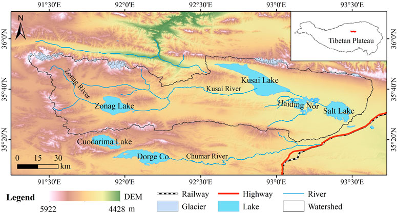
FIGURE 1. The spatial distribution of the Zonag Lake and the Salt Lake drainage basin.
The Salt Lake was primarily supplied by seasonal rivers. Until September 2011, the Salt Lake’s water volume remained stable. There are three lakes northwest of the Salt Lake: Haiding Nor, Kusai Lake, and Zonag Lake (Figure 1), which belonged to typical endorheic lakes before the outburst of the Zonag Lake in September 2011 (Liu et al., 2016). The Zonag Lake is mainly supplied by glacial melt water through the Zonag River. The Kusai River is the main water source of the Kusai Lake. The Haiding Nor is fed by the surface runoff and intermittent stream. After the outburst, the lake water flowed eastward successively through the Kusai Lake and the Haiding Nor. Finally, it flooded into the Salt Lake, resulting in the hydraulic connection of the four lakes with newly-formed channels. The Salt Lake has experienced rapid expansion since 2011. Figure 2 shows the considerable growth of the Salt Lake area from 9 November 2011 to 11 November 2012 through the Landsat seven imageries, severely threatening the engineering constructions.
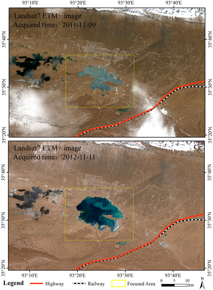
FIGURE 2. The variation of the Salt Lake (yellow box) as observed via the Landsat 7 images.
As one of the most eminent satellite series, Landsat has been observing the Earth for 50 years since 1972, which provides medium-resolution images for scientific research (Wulder et al., 2022). The Landsat eight is one of the newest Landsat satellites, and its data has been widely used for surface water detection (Donchyts et al., 2016a; Pekel et al., 2016; Albarqouni et al., 2022). Herein, the Landsat eight satellite imagery was used to obtain lake occurrences for machine learning modeling via visual interpretation. As a planetary-scale platform for geospatial analysis, Google Earth Engine (GEE) collects a large amount of remote sensing data and powerful algorithms (Gorelick et al., 2017) and was used for the preprocessing of Landsat eight satellite images in this research. Additionally, we specially prepared separate training data and testing data from different periods and regions to effectively evaluate the machine model’s ability to resist overfitting. We selected the subset of the Inner Tibetan Plateau (Inner E), where the Salt Lake is located, as the sampling location for training data. A detailed description of the area can be found in this paper (Wan et al., 2016). We obtained images with a cloud cover percentage of less than 5% in September and October in the Inner E from 2013 to 2021 and calculated the mean value of the images. Afterwards, the lakes were manually delineated and converted into sample points using the algorithm of GEE. Finally, the total number of lake points was 101,045. Likewise, we collected 124,580 non-lake points. For the testing data, the images from July to November 2020 in the central Tibetan Plateau were acquired for mosaicing, and then 537 lake points and 674 non-lake points were visually interpreted.
The feature variables are crucial for the training of machine learning models. The variables were selected considering the water characteristics and data availability. Image bands, water indices, and topographic variables were finally chosen, referring to the information in the existing literature (McFeeters, 1996; Frazier and Page, 2000; Ouma and Tateishi, 2006; Xu, 2006; Feyisa et al., 2014; Yin et al., 2021). A total of 13 feature variables were selected for surface water extraction—-namely, the blue band (B), G, R, NIR, SWIR1, SWIR2, NDWI, NDWI3, MNDWI, AWEIsh, AWEInsh, Slope, and Aspect. For quick reference, Table 1 lists the water indices mentioned above. Note that Blue, Green, NIR, SWIR1, and SWIR2 represent top-of-atmosphere reflectance for corresponding Landsat eight bands. In this paper, the Landsat five and Landsat eight images from 1986 to 2021 (except 2011 and 2012) were acquired based on the principle of low cloud cover, and the water indices were calculated through GEE. All satellite images used in the study are listed in Supplementary Table S1. Without suitable data from the satellites mentioned above, we downloaded data from satellite seven in 2011 and 2012 via the United States Geological Survey (USGS, https://earthexplorer.usgs.gov/, accessed on 3 October 2021), whose imagery was partially missing due to the Scan Line Corrector (SLC) failure. Afterwards, the partial images were interpolated locally to obtain the complete images, and the lake vector polygons were delineated through visual interpretation. In addition, we downloaded the earliest imagery covering the Salt Lake (acquired in 1973) from the USGS website and visually interpreted it. The Shuttle Radar Topography Mission (SRTM) data was employed to calculate topographic variables (i.e., Slope and Aspect).
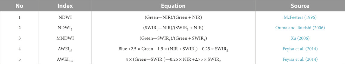
TABLE 1. Water index methods using Landsat OLI data.
In this study, we used three machine learning models–exactly CART, RF, and SVM–to extract water. Lake volume and the likelihood of lake water overflow were calculated using the SRTM data. The flowchart for the water extraction and analysis is presented in Figure 3. The main steps are described as follows.
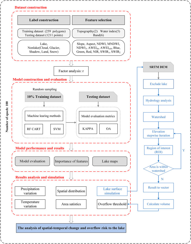
FIGURE 3. Flowchart of the proposed methodology for water extraction in this work.
1) Firstly, we constructed a lake inventory using GEE. This inventory included separate training and testing data. Five strata were introduced for better separation of lake samples from non-lake samples (i.e., cloud, glacier, shadow, land, snow). Regarding feature selection, SRTM DEM and satellite images were prepared to construct 13 feature variables. Then, Pearson’s correlation (r) was employed to assess the correlations between these variables.
2) Secondly, the training and testing data were created according to a binary variable, where one and 0 represent the lake point and non-lake point, respectively. The training data was first shuffled and then randomly sampled at a percentage ratio of 10%. The testing data was used to measure the performance of the three models. The models were run 100 times with different sample combinations using CART, RF, and SVM, and each time, the training samples were split randomly with a ratio of 10%. After the models were trained, accuracy evaluation and model comparison was performed using KAPPA and OA.
3) Thirdly, after the model capabilities were compared, evaluation metrics for the three models were calculated, the relative importance of the feature variables for the tree-based models was obtained, and the best performing model was used to extract the water body extent.
4) Finally, we conducted a spatiotemporal analysis of the Salt Lake to assess its changes from 1973 to 2021. Climate characteristics were analyzed using temperature and precipitation data. In addition, the watershed in the basin where the Salt Lake is located was derived through hydrology analysis. The maximum boundary of the Salt Lake was simulated by iterating DEM until its water overflowed the watershed. The overflow potential of the Salt Lake was assessed by calculating the increment of the water volume.
CART, RF, and SVM were employed for lake extraction by relating the lake inventory dataset to feature variables. All the machine learning algorithms were implemented using the cloud-based platform–GEE. Hydrology analysis of the Salt Lake was performed via the geographic information system (GIS) software. Detailed depictions of the three machine learning models and hydrology analysis are presented as follows.
CART belongs to a kind of Decision Trees (DTs) algorithm, which was first proposed by Breiman et al. (1984). CART is a supervised classification algorithm whose input data can be continuous or discrete variables. Unlike other decision tree algorithms (i.e., ID3, C4.5), CART can handle both classification and regression tasks (Quinlan, 1986; Salzberg, 1994). In the classification problem, a simple decision rule is learned from features in the data to develop a model that predicts the target variable. Compared to other machine learning techniques, the principle of CART is simple to understand, and its decision tree can be visualized. In addition, the input data for CART requires little data preparation, such as normalization, blank values removal, and dummy variables creation. In the process of dealing with classification problems, CART can also yield the importance of each input variable by the Gini index.
RF is an ensemble learning approach that aggregates a large number of CART decision trees to generate a single model with a more accurate prediction (Breiman, 2001). RF has been a widely used model in both classification and regression tasks (Belgiu and Drăguţ, 2016). When handling classification tasks, these CART decision trees are generated based on different subsets of the training dataset, which contain randomly selected features and samples (i.e., bootstrap sample with replacement) (Yin et al., 2021). After RF is established, samples are first evaluated individually by each decision tree in the model and then determined by the majority of those decision trees. As a frequently used bagging model, RF is resistant to overfitting by combining ensemble learning and bootstrap sample (Guan et al., 2013). Like the decision tree algorithm, RF can also generate the importance of each feature variable by the Information Gain (IG), Information Gain Ratio (IGR), or Gini index when dealing with classification problems.
SVM is one of the supervised learning methods widely used for classification and regression tasks (Cortes and Vapnik, 1995; Vapnik, 1999). The optimal classification hyperplane and the kernel function are the two central principles of SVM (Yao et al., 2008). Optimizing the classification hyperplane aims to correctly differentiate between the positive and negative samples while maximizing the classification margin. The role of the kernel function is to transform the initially non-separable data into linearly separable data in a higher dimensional feature space. During the training process, SVM can ignore outliers and focus on the maximum margin by adjusting the regularization parameter (Sarp and Ozcelik, 2017). Additionally, SVM can also effectively handle datasets with more features than samples.
In order to assess the risk of Salt Lake water overflow, the SRTM DEM was employed to construct equations between the area and the volume. In the calculation formula, ΔV represents the change of lake water volume in two periods, A1 and A2 represent the area of the lake in different periods, respectively, with lake area A1 and level H1 for the previous period and lake area A2 and level H2 for the later period. This method has been frequently used in estimating lake water volume (Liu et al., 2021; Lu et al., 2021).
Factor importance refers to the relative importance of each feature variable, indicating the role of each variable in the modeling process. Measuring the relative importance of each factor is crucial to understand the modeling process. RF can be utilized to assess the relative importance of each feature variable (Yin et al., 2021), as can CART. In this paper, the relative importance of factors was obtained according to 100 rounds of RF and CART output results, accumulating the normalized results of factor importance for the modeling in each round.
The performance of the three models was evaluated through 100 rounds of accuracy evaluation results. In this study, the extraction of the Salt Lake based on machine learning models is a classification problem with binary results of the presence and absence of lake pixels. In classification problems, a confusion matrix, which combines the actual class of the sample and the model’s predicted class, is obtained to compute evaluation metrics such as commission error and omission error (Liu et al., 2020). In this paper, the Kappa coefficient (KAPPA) and the overall accuracy (OA), derived from the confusion matrix, were mainly considered indicators to measure the overall model performance (Warrens and Pratiwi, 2016; Liu et al., 2020).
According to the accuracy evaluation results in Figure 4, the RF model had the best outcome in terms of KAPPA and OA, followed by CART and SVM. The mean KAPPA for the 100-round RF model was 0.9876, and the mean OA was 0.9939. The higher values of the two evaluation indicators mean the better accuracy of the model. As shown in Figure 4, the values of the evaluation indicators of the three models were all higher than 0.85, indicating that these models had good performance in water extraction. The distribution of the two evaluation indicators for the RF model was very concentrated, which proved that it was very stable in 100 rounds of modeling. Although the results of the two evaluation indicators showed good accuracy for the CART model, the distribution of the results was not concentrated, indicating that it was not as stable as the RF model. The SVM model had relatively low accuracy and its accuracy distribution approximated a normal distribution. After the comprehensive evaluation, the RF model was selected for the extraction of the Salt Lake.
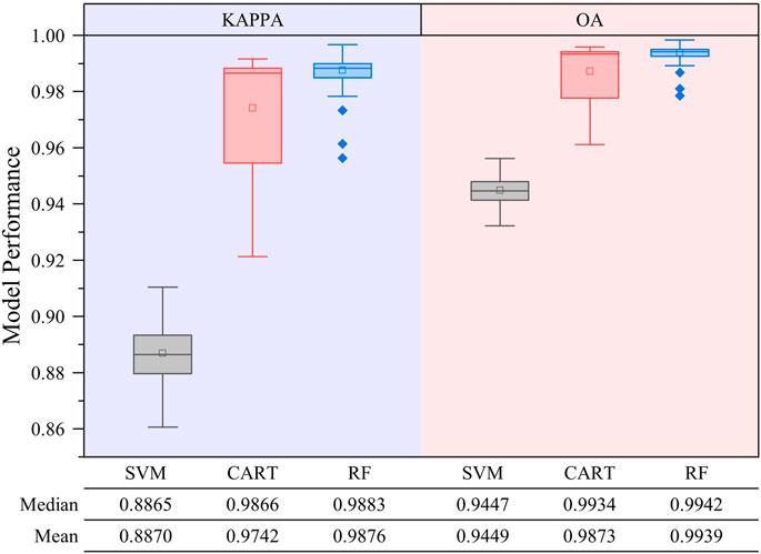
FIGURE 4. Evaluation metrics regarding the performances of different models.
In this paper, the Pearson correlation coefficient was calculated between the feature variables to check the multicollinearity of the data (Figure 5). The result shows that there was strong collinearity between the feature variables (absolute value greater than 0.7). For example, NDWI and MNDWI, which are widely employed in water body extraction, had a correlation coefficient value of 0.84, indicating that these two water indices could be used as substitutes for each other.
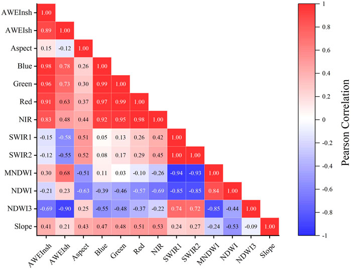
FIGURE 5. Pearson’s correlations between feature variables.
In the factor contribution analysis experiment, if there are strongly correlated feature variables, any one of them can be used as an excellent feature to participate in the construction of the model. Once one of these correlated feature variables is selected, the mean decrease impurity is occupied by this variable, resulting in the reduction of the importance of other feature variables. In order to solve this problem, we randomly sampled the training dataset to set up the machine learning models. In addition, we also accumulated the results of the machine learning models for 100 experiments because the results of a single experiment cannot indicate whether the experimental results are reliable. According to the relative importance analysis results in Figure 6, NDWI was considered the most important feature variable in the lake extraction by RF and CART models, while AWEInsh seemed to be the least important feature variable.
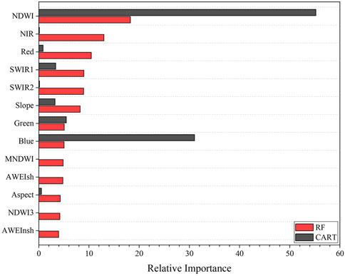
FIGURE 6. The relative importance of each feature variable from RF and CART.
The long-term evolution of the Salt Lake between 1973 and 2021 is shown in Figure 7. During the period 1973–1987, the Salt Lake area showed an enormous 53% reduction, from 41.09 in 1973 to 19.30 km2 in 1987. Until 1989, the Salt Lake area went back to its previous size. Between 1989 and 1995, the Salt Lake area declined in a linear fashion, almost to its area value in 1989. Slow growth in the Salt Lake area occurred from 1995 to 2010. After the outburst of the Zonag Lake in September 2011, the Salt Lake area reached 73.32 km2 in November 2011, showing a 57% area increase compared to the 46.54 km2 of the Salt Lake area in November 2010. From 2010 to 2019, the Salt Lake area experienced a dramatic expansion, then a steady increase, and finally a rapid expansion, and eventually, it reached a maximum area value of 209.43 km2 in 2019, showing an astonishing 350% area increase. The most recent 3 years (2019–2021) were relatively stable periods with a slight decline, possibly due to the construction of the artificial drainage channel.
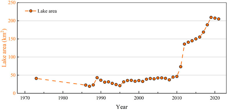
FIGURE 7. Changes in the Salt Lake area from 1973 to 2021.
Temperature and precipitation data from the nearest China meteorological station (Wudaoliang) to the Salt Lake are shown in Figure 8. Temperature observations from 1980 to 2017 revealed a warming rate of 0.05°C/a (p <0.05), with annual average temperatures almost always higher than the multi-year average temperature since 1998 (Figure 8A). Precipitation also showed an overall increasing trend (p <0.05), especially after 1996 (Figure 8B). After the collapse of the Zonag Lake (circa 2011), the Salt Lake, as a tailwater lake, was heavily recharged by the upstream lakes. Therefore, the response of the Salt Lake to climate was mainly focused on the period from 1986 to 2010. Overall, the fluctuation of precipitation matched the change in the Salt Lake area well, compared with the temperature (Figure 9). For example, high precipitation in 1989 and 2008–2010 was associated with high lake areas, whereas low precipitation from 1990 to 1995 coincided with small lake areas. Pearson’s correlation analysis was conducted between the lake area variable and the precipitation variable from 1986 to 2010. A correlation coefficient value of 0.603 (p <0.01) indicated a significant correlation between the variables.
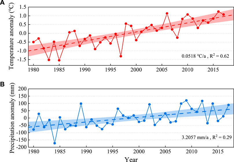
FIGURE 8. Climate variations from 1980 to 2017: (A) time series of annual average temperature change and (B) time series of annual precipitation change.
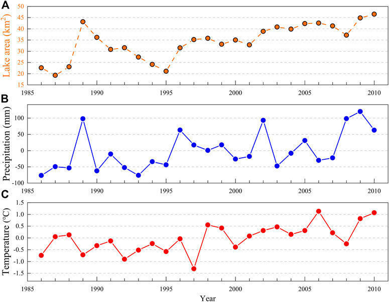
FIGURE 9. Changes in lake area and climate fluctuations from 1986 to 2010: (A) lake area, (B) precipitation and (C) temperature.
Maps of the Salt Lake in 1973 and 2010 were selected as reference data before and after the Zonag Lake outburst, and the area changes of Salt Lake in different directions were analyzed based on the geometric center of these reference maps (Figure 10). From 1973 to 2010, the Salt Lake area increased from 41.09 km2 to 46.54 km2, and the main directions of area expansion were the east, south, north, and northwest, but the area growth did not exceed 1 km2. Between 2010 and 2012, the Salt Lake, affected by the lake overflow, expanded in all directions by more than 5 km2, of which the main expansion direction was the southeast, and the expansion area reached 17.80 km2, followed by the southwest, west, and south, with an expansion area of all more than 10 km2. During the period from 2012 to 2019, the Salt Lake area reached a maximum value of 209.43 km2 and expanded in all directions, with the main orientations including southeast, south, and west. In the last 2 years (2019–2021), the area of the Salt Lake decreased slightly in all directions, with an area of no more than 1 km2.
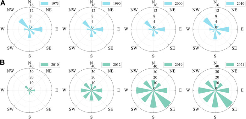
FIGURE 10. Changes in different directions of the Salt Lake before (A) and after (B) the outburst of the Zonag Lake.
The overflow condition of the Salt Lake is that its boundary crosses the watershed between the Salt Lake and Qingshui Lake, which can be simulated through the iteration of the lake water level. The water level corresponding to the inundation area was calculated as the mean value of the SRTM DEM grids intersecting the lake shoreline. To minimize the uncertainty of SRTM DEM, three times the Normalized Median Absolute Deviation (NMAD) was employed to filter out outliers (Höhle and Höhle, 2009; Leys et al., 2013). Figure 11 shows the maximum expansion area of the Salt Lake when it meets the overflow condition. The area and elevation of the overflowed Salt Lake-simulated were 220.09 km2 and 4,471.42 m, respectively. According to the lake area time series in Figure 7, the lake area changes from 2012 to 2019 were selected to assess the risk of Salt Lake water overflow. In the case of slow growth in the area of the Salt Lake (from 2012 to 2016), the water level continued to rise at a vertical rate of 0.84 m/a (0.12 billion m3/a), and the water level is predicted to reach its watershed overflow elevation of 4,471.4 m by 2031 (assuming the 0.12 billion m3/a rate keeps the same). From 2016 to 2019, the water level of the Salt Lake rose rapidly at a rate of 2.96 m/a (0.54 billion m3/a), and the Salt Lake is projected to reach its maximum water capacity in 2020. Fortunately, the emergency drainage channel between the Salt Lake and Qingshui Lake was completed in 2019 (Figure 11) (Lu et al., 2021). Since then, this artificial channel has been connected with the tributary of the Yangtze River, resulting in the endorheic-exorheic transition of the Salt Lake catchment.
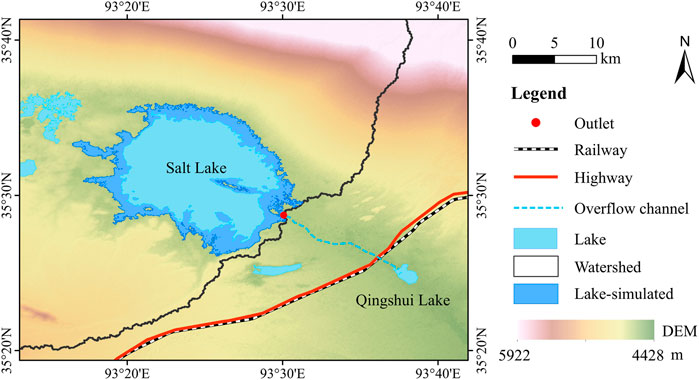
FIGURE 11. The maximum expansion area of the Salt Lake before overflow.
The three applied methods, CART, RF, and SVM, are very popular machine learning methods in the field of earth sciences (Huang et al., 2015; Donchyts et al., 2016b; Liu et al., 2020). In this paper, the results showed that tree-based algorithms, especially the RF model, outperformed the SVM model in terms of KAPPA and OA, and the excellent capability of the RF model has been facilitated by other studies (Huang et al., 2015; Belgiu and Drăguţ, 2016). Compared with the SVM model, tree-based models (i.e., CART and RF) can directly output the importance order of feature variables, which can help researchers explore the relationship between feature variables and target variables. The difference between SVM and tree-based models is mainly the basic framework. SVM is developed from statistical learning theory, with structural risk minimization as its principle (Chapelle et al., 1999). SVM is appropriate for image classification with a small number of training samples and a high-dimensional feature space (Melgani and Bruzzone, 2004). Tree-based algorithms, one of the most frequently used supervised classification methods (Rokach and Maimon, 2005; Belgiu and Drăguţ, 2016), have multiple interior nodes and leaf nodes, representing the feature and target variables, respectively (Huang et al., 2015).
In this study, both the CART algorithm and RF algorithm had high accuracy and output the importance ranking of feature variables. There are two differences between the two algorithms: one is that the results of the RF algorithm were more robust, and the other is that the relative importance results of the RF algorithm were more reasonable without the bias of feature variables. This is because the RF method is based on the idea of ensemble learning, integrates multiple decision trees to construct a model, and has two aspects of randomness. In comparison to a single decision tree, it can improve prediction accuracy (Ho, 1998). Taking multiple aspects of the model into consideration, RF is recommended for the extraction of lakes in the Hoh Xil region.
Since the lake outburst event in 2011, the four lakes (i.e., the Salt Lake, Haiding Nor, Kusai Lake, and Zonag Lake) have been hydrologically connected with newly-formed channels (Liu W. et al., 2019). Although these reorganization events occurred in the endorheic basins, the results showed that the significant increase in the Salt Lake water volume could overflow to the adjacent exorheic basin, seriously threatening the engineering construction. In the worst-case scenario, the outburst flood from Salt Lake can destroy engineering infrastructure within 6 hours (Liu et al., 2021). In the end, to reduce the impact of the potential Salt Lake outburst, the local government constructed a drainage channel to divert the lake water into the Qingshui River, which also led to the endorheic-exorheic transition (Lu et al., 2021).
The construction of the emergency drainage channel can reduce the potential damage of an outburst flood, and the impact of the endorheic-exorheic transition requires special attention. The highly mineralized lake water is continuously discharged into the Qingshui River, which not only influences the stability of the permafrost around the water system but also impacts the northernmost source of the Yangtze River water quality (Liu M. et al., 2019; Liu et al., 2021; Lu et al., 2021). In addition, studies have shown that the total area of lakes on the Inner Tibetan Plateau will continue to expand from 2016 to 2035 (Yang et al., 2018; Zhang et al., 2020). Therefore, it is indispensable to monitor whether the drainage of the artificial channel is sufficient to cope with the large amount of water from the Salt Lake. Further, it is necessary to consider whether there are similar cases in other basins.
In this work, three machine learning models were implemented 1,000 times to compare performance using different subsets of the training dataset. Finally, the best performing random forest model was trained using 70% of the entire training data and applied to the long-term lake extraction. The current research also has some limitations. Our study area is located on the QTP, where there is less human activity. For this reason, the training samples were selected on the QTP, and the machine learning model was trained using these samples. Therefore, the results of the relative importance of features may not be suitable for lakes in urban areas.
The QTP is distributed in numerous lakes, which are an important part of the Asian Water Tower (Zhang et al., 2021; Yao et al., 2022). These lakes are subject to little human intervention and respond exceptionally quickly to climate change (Zhang et al., 2020). Abnormal climate events such as El Niño and La Niña significantly impact the global climate. However, the response of lakes on the QTP to abnormal climate events is less involved (Lei et al., 2019). In addition, water system reorganization events are expected to increase by 20 from 2019 to 2030 (Liu et al., 2021), and these accelerated evolutions and impacts should be continuously monitored and confirmed in future work. Currently, research on lake area changes on the QTP mainly focuses on inter-annual changes (Zhang et al., 2020; 2021). With the launch of remote sensing satellites in the future, the intra-annual variations of the lake should be studied to understand its response to climate change better.
In this study, we used machine learning models to extract the Salt Lake area in the Hoh Xil region. Meanwhile, based on the long-term lake area data, we analyzed its response to meteorological data and simulated the Salt Lake water overflow scenario. The conclusions are as follows.
1) This study used KAPPA and OA to evaluate model performance and found out that RF is the best performing model compared to CART and SVM. The mean accuracy of KAPPA and OA for the 100-round RF model were 0.9876 and 0.9939, respectively.
2) There was a strong correlation between most water indices. Through the factor contribution analysis, it was found that NDWI was the most important feature selected by RF and CART for the area extraction of the Salt Lake.
3) Before the Zonag Lake outburst, the area change of the Salt Lake was consistent with the variation of precipitation, and the correlation coefficient value reached 0.603. After that, the area of the Salt Lake expanded at an alarming rate in all orientations, and the primary expansion directions were southeast, west, southwest, and south.
4) The area of the overflowed Salt Lake-simulated was 220.09 km2. The simulation result indicated that the earliest and latest times for the Salt Lake to overflow were 2020 and 2031, respectively.
The results of this paper improve the understanding of the impact of water system reorganization on downstream lakes. Continued research in this region is required due to the endorheic-exorheic transition in the future. In addition, the intra-annual variation of the Salt Lake needs to be considered, and the reasons for the variation need to be quantitatively analyzed. Herein, we suggest that other areas of the QTP with water system reorganization need to be studied to gain a better understanding and reduce the disasters caused by lake outbursts.
The raw data supporting the conclusion of this article will be made available by the authors, without undue reservation.
RW, LG and JL contributed to conception and design of the study. RW, BC and YY processed and analyzed data. RW wrote the first draft of the manuscript. HZ and FD wrote sections of the manuscript. All authors have read and agreed to the published version of the manuscript.
This research was funded by the Second Tibetan Plateau Scientific Expedition and Research Program (STEP, Grant No. 2019QZKK0906).
We would like to thank the editor and reviewers for their suggestions.
The authors declare that the research was conducted in the absence of any commercial or financial relationships that could be construed as a potential conflict of interest.
All claims expressed in this article are solely those of the authors and do not necessarily represent those of their affiliated organizations, or those of the publisher, the editors and the reviewers. Any product that may be evaluated in this article, or claim that may be made by its manufacturer, is not guaranteed or endorsed by the publisher.
The Supplementary Material for this article can be found online at: https://www.frontiersin.org/articles/10.3389/feart.2022.1084540/full#supplementary-material
Albarqouni, M. M. Y., Yagmur, N., Bektas Balcik, F., and Sekertekin, A. (2022). Assessment of spatio-temporal changes in water surface extents and lake surface temperatures using google earth engine for lakes region, türkiye. Int. J. Geo-Inf. 11, 407. doi:10.3390/ijgi11070407
Belgiu, M., and Drăguţ, L. (2016). Random forest in remote sensing: A review of applications and future directions. Isprs J. Photogramm. 114, 24–31. doi:10.1016/j.isprsjprs.2016.01.011
Bijeesh, T. V., and Narasimhamurthy, K. N. (2020). Surface water detection and delineation using remote sensing images: A review of methods and algorithms. Sustain. Water Resour. Manag. 6, 68. doi:10.1007/s40899-020-00425-4
Breiman, L., Friedman, J. H., Olshen, R. A., and Stone, C. J. (1984). Classification and regression trees (CART). Biometrics 40, 358.
Chapelle, O., Haffner, P., and Vapnik, V. (1999). Support vector machines for histogram-based image classification. IEEE Trans. Neural Netw. 10, 1055–1064. doi:10.1109/72.788646
Chen, D., Xu, B., Yao, T., Guo, Z., Cui, P., Chen, F., et al. (2015). Assessment of past, present and future environmental changes on the Tibetan Plateau. Chin. Sci. Bull. 60, 3025–3035. doi:10.1360/N972014-01370
Cortes, C., and Vapnik, V. (1995). Support-vector networks. Mach. Learn. 20, 273–297. doi:10.1007/BF00994018
Domenikiotis, C., Loukas, A., and Dalezios, N. R. (2003). The use of NOAA/AVHRR satellite data for monitoring and assessment of forest fires and floods. Nat. Hazard Earth Syst. 3, 115–128. doi:10.5194/nhess-3-115-2003
Donchyts, G., Baart, F., Winsemius, H., Gorelick, N., Kwadijk, J., and van de Giesen, N. (2016a). Earth’s surface water change over the past 30 years. Nat. Clim. Change 6, 810–813. doi:10.1038/nclimate3111
Donchyts, G., Schellekens, J., Winsemius, H., Eisemann, E., and van de Giesen, N. (2016b). A 30 m resolution surface water mask including estimation of positional and thematic differences using landsat 8, SRTM and OpenStreetMap: A case study in the murray-darling basin, Australia. Remote Sens-Basel 8, 386. doi:10.3390/rs8050386
Feyisa, G. L., Meilby, H., Fensholt, R., and Proud, S. R. (2014). Automated water extraction index: A new technique for surface water mapping using landsat imagery. Remote Sens. Environ. 140, 23–35. doi:10.1016/j.rse.2013.08.029
Ficklin, D. L., Abatzoglou, J. T., and Novick, K. A. (2019). A new perspective on terrestrial hydrologic intensity that incorporates atmospheric water demand. Geophys Res. Lett. 46, 8114–8124. doi:10.1029/2019GL084015
Fisher, A. (2016). Comparing Landsat water index methods for automated water classification in eastern Australia. Remote Sens. Environ. 175, 167–182. doi:10.1016/j.rse.2015.12.055
Frazier, P. S., and Page, K. J. (2000). Water body detection and delineation with landsat TM data. Photogramm. Eng. 66, 1461–1467.
Gorelick, N., Hancher, M., Dixon, M., Ilyushchenko, S., Thau, D., and Moore, R. (2017). Google earth engine: Planetary-scale geospatial analysis for everyone. Remote Sens. Environ. 202, 18–27. doi:10.1016/j.rse.2017.06.031
Guan, H., Li, J., Chapman, M., Deng, F., Ji, Z., and Yang, X. (2013). Integration of orthoimagery and lidar data for object-based urban thematic mapping using random forests. Int. J. Remote Sens. 34, 5166–5186. doi:10.1080/01431161.2013.788261
Ho, T. K. (1998). The random subspace method for constructing decision forests. IEEE T Pattern Anal. 20, 832–844. doi:10.1109/34.709601
Höhle, J., and Höhle, M. (2009). Accuracy assessment of digital elevation models by means of robust statistical methods. Isprs J. Photogramm. 64, 398–406. doi:10.1016/j.isprsjprs.2009.02.003
Huang, X., Xie, C., Fang, X., and Zhang, L. (2015). Combining pixel- and object-based machine learning for identification of water-body types from urban high-resolution remote-sensing imagery. IEEE J-Stars 8, 2097–2110. doi:10.1109/JSTARS.2015.2420713
Huang, C., Chen, Y., Zhang, S., and Wu, J. (2018). Detecting, extracting, and monitoring surface water from space using optical sensors: A review. Rev. Geophys. 56, 333–360. doi:10.1029/2018RG000598
Huntington, T. G., Weiskel, P. K., Wolock, D. M., and McCabe, G. J. (2018). A new indicator framework for quantifying the intensity of the terrestrial water cycle. J. Hydrol. 559, 361–372. doi:10.1016/j.jhydrol.2018.02.048
Huntington, T. G. (2006). Evidence for intensification of the global water cycle: Review and synthesis. J. Hydrol. 319, 83–95. doi:10.1016/j.jhydrol.2005.07.003
Isikdogan, L. F., Bovik, A., and Passalacqua, P. (2020). Seeing through the clouds with DeepWaterMap. IEEE Geosci. Remote S 17, 1662–1666. doi:10.1109/LGRS.2019.2953261
Jain, S. K., Singh, R. D., Jain, M. K., and Lohani, A. K. (2005). Delineation of flood-prone areas using remote sensing techniques. Water Resour. Manag. 19, 333–347. doi:10.1007/s11269-005-3281-5
Ji, L., Zhang, L., and Wylie, B. K. (2009). Analysis of dynamic thresholds for the normalized difference water index. Photogramm. Eng. Rem. S 75, 1307–1317. doi:10.14358/PERS.75.11.1307
Lei, Y., Zhu, Y., Wang, B., Yao, T., Yang, K., Zhang, X., et al. (2019). Extreme Lake level changes on the Tibetan plateau associated with the 2015/2016 El Niño. Geophys Res. Lett. 46, 5889–5898. doi:10.1029/2019GL081946
Leys, C., Ley, C., Klein, O., Bernard, P., and Licata, L. (2013). Detecting outliers: Do not use standard deviation around the mean, use absolute deviation around the median. J. Exp. Soc. Psychol. 49, 764–766. doi:10.1016/j.jesp.2013.03.013
Li, Y., and Niu, Z. (2022). Systematic method for mapping fine-resolution water cover types in China based on time series Sentinel-1 and 2 images. Int. J. Appl. Earth Obs. 106, 102656. doi:10.1016/j.jag.2021.102656
Liu, B., Li, L., Du, Y., Liang, T., Duan, S., Hou, F., et al. (2016). Causes of the outburst of Zonag Lake in Hoh Xil, Tibetan plateau, and its impact on surrounding environment. J. Glaciol. Geocryol. 38, 305. doi:10.7522/j.issn.1000-0240.2016.0033
Liu, M., Zhao, W., Wang, Q., Huang, S., and Shi, K. (2019). Compatibility issues with irregular current injection islanding detection methods and a solution. Energies 12, 1467. doi:10.3390/en12081467
Liu, W., Xie, C., Zhao, L., Wu, T., Wang, W., Zhang, Y., et al. (2019). Dynamic changes in lakes in the Hoh Xil region before and after the 2011 outburst of Zonag Lake. J. Mt. Sci-Engl 16, 1098–1110. doi:10.1007/s11629-018-5085-0
Liu, Q., Huang, C., Shi, Z., and Zhang, S. (2020). Probabilistic river water mapping from landsat-8 using the support vector machine method. Remote Sens-Basel 12, 1374. doi:10.3390/rs12091374
Liu, K., Ke, L., Wang, J., Jiang, L., Richards, K. S., Sheng, Y., et al. (2021). Ongoing drainage reorganization driven by rapid lake growths on the Tibetan plateau. Geophys Res. Lett. 48, e2021GL095795. doi:10.1029/2021GL095795
Lu, D., and Weng, Q. (2007). A survey of image classification methods and techniques for improving classification performance. Int. J. Remote Sens. 28, 823–870. doi:10.1080/01431160600746456
Lu, P., Han, J., Li, Z., Xu, R., Li, R., Hao, T., et al. (2020). Lake outburst accelerated permafrost degradation on Qinghai-Tibet Plateau. Remote Sens. Environ. 249, 112011. doi:10.1016/j.rse.2020.112011
Lu, S., Jin, J., Zhou, J., Li, X., Ju, J., Li, M., et al. (2021). Drainage basin reorganization and endorheic-exorheic transition triggered by climate change and human intervention. Glob. Planet Change 201, 103494. doi:10.1016/j.gloplacha.2021.103494
Ma, R., Yang, G., Duan, H., Jiang, J., Wang, S., Feng, X., et al. (2011). China’s lakes at present: Number, area and spatial distribution. Sci. China Earth Sci. 54, 283–289. doi:10.1007/s11430-010-4052-6
Manaf, S. A., Mustapha, N., Sulaiman, M. N., Husin, N. A., and Hamid, M. R. A. (2016). Comparison of classification techniques on fused optical and SAR images for shoreline extraction: A case study at northeast coast of peninsular Malaysia. J. Comput. Sci. 12, 399–411. doi:10.3844/jcssp.2016.399.411
McFeeters, S. K. (1996). The use of the Normalized Difference Water Index (NDWI) in the delineation of open water features. Int. J. Remote Sens. 17, 1425–1432. doi:10.1080/01431169608948714
Melgani, F., and Bruzzone, L. (2004). Classification of hyperspectral remote sensing images with support vector machines. IEEE T Geosci. Remote 42, 1778–1790. doi:10.1109/TGRS.2004.831865
Milner, A. M., Khamis, K., Battin, T. J., Brittain, J. E., Barrand, N. E., Füreder, L., et al. (2017). Glacier shrinkage driving global changes in downstream systems. Proc. Natl. Acad. Sci. 114, 9770–9778. doi:10.1073/pnas.1619807114
Ouma, Y. O., and Tateishi, R. (2006). A water index for rapid mapping of shoreline changes of five East African Rift Valley lakes: An empirical analysis using Landsat TM and ETM+ data. Int. J. Remote Sens. 27, 3153–3181. doi:10.1080/01431160500309934
Paul, A., Tripathi, D., and Dutta, D. (2018). Application and comparison of advanced supervised classifiers in extraction of water bodies from remote sensing images. Sustain. Water Resour. Manag. 4, 905–919. doi:10.1007/s40899-017-0184-6
Pekel, J.-F., Cottam, A., Gorelick, N., and Belward, A. S. (2016). High-resolution mapping of global surface water and its long-term changes. Nature 540, 418–422. doi:10.1038/nature20584
Ran, Y., Li, X., and Cheng, G. (2018). Climate warming over the past half century has led to thermal degradation of permafrost on the Qinghai–Tibet Plateau. Cryosphere 12, 595–608. doi:10.5194/tc-12-595-2018
Rokach, L., and Maimon, O. (2005). Top-down induction of decision trees classifiers - a survey. IEEE Trans. Syst. Man, Cybern. Part C Appl. Rev. 35, 476–487. doi:10.1109/TSMCC.2004.843247
Rokni, K., Ahmad, A., Solaimani, K., and Hazini, S. (2015). A new approach for surface water change detection: Integration of pixel level image fusion and image classification techniques. Int. J. Appl. Earth Obs. 34, 226–234. doi:10.1016/j.jag.2014.08.014
Rundquist, D. C., Lawson, M. P., Queen, L. P., and Cerveny, R. S. (1987). The relationship between summer-season rainfall events and lake-surface AREA1. JAWRA J. Am. Water Resour. Assoc. 23, 493–508. doi:10.1111/j.1752-1688.1987.tb00828.x
Salzberg, S. L. (1994). C4.5: Programs for machine learning by J. Ross quinlan. Mach. Learn. 16, 235–240. doi:10.1007/BF00993309
Sarp, G., and Ozcelik, M. (2017). Water body extraction and change detection using time series: A case study of lake burdur, Turkey. J. Taibah Univ. Sci. 11, 381–391. doi:10.1016/j.jtusci.2016.04.005
Shean, D. E., Bhushan, S., Montesano, P., Rounce, D. R., Arendt, A., and Osmanoglu, B. (2020). A systematic, regional assessment of high mountain Asia glacier mass balance. Front. Earth Sci. 7, 363. doi:10.3389/feart.2019.00363
Shen, C., Laloy, E., Elshorbagy, A., Albert, A., Bales, J., Chang, F.-J., et al. (2018). HESS Opinions: Incubating deep-learning-powered hydrologic science advances as a community. Hydrol. Earth Syst. S. C. 22, 5639–5656. doi:10.5194/hess-22-5639-2018
Subin, Z. M., Riley, W. J., and Mironov, D. (2012). An improved lake model for climate simulations: Model structure, evaluation, and sensitivity analyses in CESM1. J. Adv. Model Earth Syst. 4, M02001. doi:10.1029/2011MS000072
Tao, S., Fang, J., Zhao, X., Zhao, S., Shen, H., Hu, H., et al. (2015). Rapid loss of lakes on the Mongolian Plateau. P Natl. Acad. Sci. U. S. A. 112, 2281–2286. doi:10.1073/pnas.1411748112
Townshend, J. R., and Justice, C. (1986). Analysis of the dynamics of African vegetation using the normalized difference vegetation index. Int. J. Remote Sens. 7, 1435–1445. doi:10.1080/01431168608948946
Vapnik, V. N. (1999). An overview of statistical learning theory. IEEE Trans. neural Netw. 10, 988–999. doi:10.1109/72.788640
Veh, G., Korup, O., and Walz, A. (2020). Hazard from Himalayan glacier lake outburst floods. Proc. Natl. Acad. Sci. 117, 907–912. doi:10.1073/pnas.1914898117
Vorosmarty, C. J., Green, P., Salisbury, J., and Lammers, R. B. (2000). Global water resources: Vulnerability from climate change and population growth. Science 289, 284–288. doi:10.1126/science.289.5477.284
Wan, W., Long, D., Hong, Y., Ma, Y., Yuan, Y., Xiao, P., et al. (2016). A lake data set for the Tibetan Plateau from the 1960s, 2005, and 2014. Sci. Data 3, 160039. doi:10.1038/sdata.2016.39
Wang, C., Jia, M., Chen, N., and Wang, W. (2018). Long-term surface water dynamics analysis based on landsat imagery and the Google Earth engine platform: A case study in the middle Yangtze River basin. Remote Sens-Basel 10, 1635. doi:10.3390/rs10101635
Wang, L., Du, Z., Wei, Z., Xu, Q., Feng, Y., Lin, P., et al. (2021). High methane emissions from thermokarst lakes on the Tibetan Plateau are largely attributed to ebullition fluxes. Sci. Total Environ. 801, 149692. doi:10.1016/j.scitotenv.2021.149692
Warrens, M. J., and Pratiwi, B. C. (2016). Kappa coefficients for circular classifications. J. Classif. 33, 507–522. doi:10.1007/s00357-016-9217-3
Work, E. A., and Gilmer, D. S. (1976). Utilization of satellite data for inventorying prairie ponds and lakes. Photogramm. Eng. Remote Sens. 42, 685–694.
Wu, Q., and Niu, F. (2013). Permafrost changes and engineering stability in Qinghai-Xizang Plateau. Chin. Sci. Bull. 58, 1079–1094. doi:10.1007/s11434-012-5587-z
Wulder, M. A., Roy, D. P., Radeloff, V. C., Loveland, T. R., Anderson, M. C., Johnson, D. M., et al. (2022). Fifty years of Landsat science and impacts. Remote Sens. Environ. 280, 113195. doi:10.1016/j.rse.2022.113195
Xu, H. (2006). Modification of normalised difference water index (NDWI) to enhance open water features in remotely sensed imagery. Int. J. Remote Sens. 27, 3025–3033. doi:10.1080/01431160600589179
Yang, K., Lu, H., Yue, S., Zhang, G., Lei, Y., La, Z., et al. (2018). Quantifying recent precipitation change and predicting lake expansion in the Inner Tibetan Plateau. Clim. Change 147, 149–163. doi:10.1007/s10584-017-2127-5
Yang, L., Driscol, J., Sarigai, S., Wu, Q., Chen, H., and Lippitt, C. D. (2022). Google Earth engine and artificial intelligence (AI): A comprehensive review. Remote Sens-Basel 14, 3253. doi:10.3390/rs14143253
Yao, X., Tham, L., and Dai, F. (2008). Landslide susceptibility mapping based on support vector machine: A case study on natural slopes of Hong Kong, China. Geomorphology 101, 572–582. doi:10.1016/j.geomorph.2008.02.011
Yao, T., Thompson, L., Yang, W., Yu, W., Gao, Y., Guo, X., et al. (2012). Different glacier status with atmospheric circulations in Tibetan Plateau and surroundings. Nat. Clim. Change 2, 663–667. doi:10.1038/nclimate1580
Yao, X., Liu, S., Sun, M., Guo, W., and Zhang, X. (2012). Changes of Kusai Lake in Hoh Xil region and causes of its water overflowing. Acta Geogr. Sin. 67, 689. doi:10.11821/xb201205011
Yao, X., Sun, M., Gong, P., Liu, B., Li, X., An, L., et al. (2018). Overflow probability of the Salt Lake in Hoh Xil region. J. Geogr. Sci. 28, 647–655. doi:10.1007/s11442-018-1496-7
Yao, T., Bolch, T., Chen, D., Gao, J., Immerzeel, W., Piao, S., et al. (2022). The imbalance of the Asian water tower. Nat. Rev. Earth Environ. 3, 618–632. doi:10.1038/s43017-022-00299-4
Yin, G., Luo, J., Niu, F., Zhou, F., Meng, X., Lin, Z., et al. (2021). Spatial analyses and susceptibility modeling of thermokarst lakes in permafrost landscapes along the Qinghai–Tibet engineering corridor. Remote Sens-Basel 13, 1974. doi:10.3390/rs13101974
Zhang, G., Zheng, G., Gao, Y., Xiang, Y., Lei, Y., and Li, J. (2017). Automated water classification in the Tibetan plateau using Chinese GF-1 WFV data. Photogramm. Eng. Rem. S 83, 509–519. doi:10.14358/PERS.83.7.509
Zhang, F., Li, J., Zhang, B., Shen, Q., Ye, H., Wang, S., et al. (2018). A simple automated dynamic threshold extraction method for the classification of large water bodies from landsat-8 OLI water index images. Int. J. Remote Sens. 39, 3429–3451. doi:10.1080/01431161.2018.1444292
Zhang, G., Luo, W., Chen, W., and Zheng, G. (2019). A robust but variable lake expansion on the Tibetan Plateau. Sci. Bull. 64, 1306–1309. doi:10.1016/j.scib.2019.07.018
Zhang, G., Yao, T., Xie, H., Yang, K., Zhu, L., Shum, C., et al. (2020). Response of Tibetan Plateau lakes to climate change: Trends, patterns, and mechanisms. Earth-Sci Rev. 208, 103269. doi:10.1016/j.earscirev.2020.103269
Zhang, G., Ran, Y., Wan, W., Luo, W., Chen, W., Xu, F., et al. (2021). 100 years of lake evolution over the Qinghai–Tibet Plateau. Earth Syst. Sci. Data 13, 3951–3966. doi:10.5194/essd-13-3951-2021
Zhang, Y., Xie, C., Wu, T., Zhao, L., Wu, J., Wu, X., et al. (2022). New permafrost is forming on the exposed bottom of Zonag Lake on the Qinghai-Tibet Plateau. Sci. Total Environ. 815, 152879. doi:10.1016/j.scitotenv.2021.152879
Keywords: Salt Lake, spatiotemporal variation, overflow risk, remote sensing, machine learning
Citation: Wang R, Guo L, Chen B, Yang Y, Zheng H, Deng F and Liu J (2023) Spatiotemporal variations and overflow risk analysis of the Salt Lake in the Hoh Xil Region using machine learning methods. Front. Earth Sci. 10:1084540. doi: 10.3389/feart.2022.1084540
Received: 30 October 2022; Accepted: 28 December 2022;
Published: 18 January 2023.
Edited by:
Xiuping Li, Institute of Tibetan Plateau Research (CAS), ChinaReviewed by:
Yufeng Dai, Institute of Tibetan Plateau Research (CAS), ChinaCopyright © 2023 Wang, Guo, Chen, Yang, Zheng, Deng and Liu. This is an open-access article distributed under the terms of the Creative Commons Attribution License (CC BY). The use, distribution or reproduction in other forums is permitted, provided the original author(s) and the copyright owner(s) are credited and that the original publication in this journal is cited, in accordance with accepted academic practice. No use, distribution or reproduction is permitted which does not comply with these terms.
*Correspondence: Jifu Liu, bGl1amlmdUBibnUuZWR1LmNu
Disclaimer: All claims expressed in this article are solely those of the authors and do not necessarily represent those of their affiliated organizations, or those of the publisher, the editors and the reviewers. Any product that may be evaluated in this article or claim that may be made by its manufacturer is not guaranteed or endorsed by the publisher.
Research integrity at Frontiers
Learn more about the work of our research integrity team to safeguard the quality of each article we publish.