Rapid construction of Rayleigh wave dispersion curve based on deep learning

Introduction: The dispersion curve of the Rayleigh-wave phase velocity (VR) is widely utilized to determine site shear-wave velocity (Vs) structures from a distance of a few metres to hundreds of metres, even on a ten-kilometre crustal scale. However, the traditional theoretical-analytical methods for calculating VRs of a wide frequency range are time-consuming because numerous extensive matrix multiplications, transfer matrix iterations and the root searching of the secular dispersion equation are involved. It is very difficult to model site structures with many layers and apply them to a population-based inversion algorithm for which many populations of multilayers forward modelling and many generations of iterations are essential.

Method: In this study, we propose a deep learning method for constructing the VR dispersion curve in a horizontally layered site with great efficiency. A deep neural network (DNN) based on the fully connected dense neural network is designed and trained to directly learn the relationships between Vs structures and dispersion curves. First, the training and validation sets are generated randomly according to a truncated Gaussian distribution, in which the mean and variance of the Vs models are statistically analysed from different regions’ empirical relationships between soil Vs and its depth. To be the supervised dataset, the corresponding VRs are calculated by the generalized reflection-transmission (R/T) coefficient method. Then, the Bayesian optimization (BO) is designed and trained to seek the optimal architecture of the deep neural network, such as the number of neurons and hidden layers and their combinations. Once the network is trained, the dispersion curve of VR can be constructed instantaneously without building and solving the secular equation.

Results and Discussion: The results show that the DNN-BO achieves a coefficient of determination (R²) and MAE for the training and validation sets of 0.98 and 8.30 and 0.97 and 8.94, respectively, which suggests that the rapid method has satisfactory generalizability and stability. The DNN-BO method accelerates the dispersion curve calculation by at least 400 times, and there is almost no increase in computation expense with an increase in soil layers.

1 Introduction

Rayleigh waves are formed by the interaction of incident P and SV plane waves at the free surface and travel parallel to that surface. The phase velocity (VR) dispersion curve of the Rayleigh wave depends on the medium parameters, such as the layer thickness and the P and S velocities. Longer wavelength Rayleigh waves penetrate deeper than shorter wavelengths over layered geologies. This dispersive behavior makes Rayleigh waves a valuable tool for determining the shear-wave velocity (Vs) of individual site structures from a distance of a few meters to hundreds of meters, even at the 10-km crustal scale of a region. Determining dispersive behavior is one of the key steps in calculating the theoretical phase velocity dispersion curve of Rayleigh waves in inverted geological structures, modeling regional Rayleigh waves and synthesizing seismograms.

To construct the dispersion curve, it is necessary to build a secular equation based on elastic wave theory and surface boundary determinations and compute its roots as a function of its frequency. The most famous method is the Thomson–Haskell algorithm (also called the transfer matrix method) (Thomson, 1950; Haskell, 1953). In the Thomson–Haskell algorithm, the dispersion equation is constructed by a sequence of matrix multiplications involving terms that are transcendental functions of the material properties of the layered medium. Many researchers have modified this method throughout the years (Schwab and Knopoff, 1970; Schwab and Knopoff, 1972; Abo-Zena, 1979; Fan et al., 2002) to improve its numerical stability and efficiency by reducing the dimension of transfer matrices and simplifying the iterative multiplication.

Another important class of algorithms for solving Rayleigh wave eigenvalue problems is the reflection and transmission coefficients (R/T) method (Kennett, 1974; Kennett and Kerry, 1979; Kennett and Clarke, 1983). The Rayleigh dispersion equation for a stratified medium is iteratively established by reflection and transmission matrices using R/T coefficients. Subsequently, this method was also modified and improved by other researchers (Luco and Apsel, 1983; Chen, 1993; Hisada, 1994; 1995; He and Chen, 2006; Pan et al., 2022).

Numerical techniques can also be used to solve the Rayleigh eigenvalue problem, including the finite difference method (Boore, 1972), numerical integration (Takeuchi and Saito, 1972), the boundary element method (Manolis and Beskos, 1988; Aung and Leong, 2010), and the spectral element method (Faccioli et al., 1996; Komatitsch and Vilotte, 1998). Although these methods have several advantages, they require more computation time.

In conventional methods, most efforts to calculate the dispersion curve are primarily focused on building the dispersion equation and searching for its phase velocity solution as a function of frequency. The computational efficiency is improved by reducing the dimension of the transfer matrix and/or simplifying the iteration of the dispersion equation. However, tedious matrix iteration and root searching cannot be avoided.

In inversion analysis, the velocity structure is estimated by minimizing the deviation between the theoretical and experimental dispersion curves. For population-based inversion algorithms, many populations of multilayer forward modeling and many generations of iterations are essential to search the optimal site parameters (shear wave velocity, overburden thickness, etc.). It is difficult to model site structures that have many layers and apply population-based inversion algorithms (Picozzi and Albarello, 2007; Lu et al., 2016; Poormirzaee, 2016; Lei et al., 2019; Poormirzaee and Fister, 2021). Therefore, it is necessary to develop a fast, accurate, stable dispersion curve construction method.

The increasing number of populations and the requirement of refining the site layers induce tremendous iteration calculation costs in the population-based inversion algorithm. Under these situations, conventional forward methods struggle to satisfy the big data processes. Deep learning (DL) techniques are one of the most potent ways to establish a good mapping relationship between the seismic signals and geophysical parameters. Once a DL model is trained, it can map the site velocity structure to the Rayleigh dispersion curve directly and quickly under similar geological conditions. The DL method has been widely applied in various geotechnical earthquake engineering applications to replace the complex conventional numerical calculation method. Jo et al. (2022) used a trained deep neural network (DNN) to replace the conventional history matching method, greatly reducing the computational cost of predicting well responses, such as oil production rate, water production rate, and reservoir flow direction. Wamriew et al. (2022) used a trained convolutional neural network to improve the efficiency and accuracy of microseismic event monitoring. Their model avoids the shortcoming that the conventional methods, which are affected by manual intervention and require substantial data preprocessing, rely on. Tschannen et al. (2022) accelerated the compilation speed in wavelet extraction through deep learning, which restrains the iterative adjustment parameters and potential noise. Similarly, some researchers in surface wave exploration have applied deep learning to extract dispersion curves (Alyousuf et al., 2018; Zhang et al., 2020; Dai et al., 2021) and invert velocity structures (Aleardi and Stucchi, 2021; Fu et al., 2021; Luo et al., 2022). Alyousuf et al. (2018) used a fully connected network to extract the fundamental-mode dispersion curve. Zhang et al. (2020) presented a convolution network to automatically extract dispersion curves. Dai et al. (2021) developed a DCNet deep learning model that can correctly extract the multimode dispersion curve from the segmentation dispersion image. Fu et al. (2021) applied DispINets to inverse the shear velocity from the multimode dispersion curve. Aleardi and Stucchi (2021) proposed a Monte Carlo-based hybrid neural network to resolve the degradation shortcomings in the inversions. Luo et al. (2022) used a DNN to investigate the range of the initial model and the reliability of the shear velocity structure. Through these successful applications, deep learning techniques have demonstrated their potential in constructing dispersion curves from site data with high efficiency.

Deep learning-based surface wave exploration research may be defined as a systematic process that consists of two essential components. One is establishing a sufficient and reasonably distributed dataset that includes all the geophysical states (Alwosheel et al., 2018). Another is designing a network that has high accuracy and efficiency. However, no one dataset ensures that the site structures of different regions are covered. Researchers (Chauhan and Dhingra, 2012; Assi et al., 2018; Itano et al., 2018) rely on the mathematical understanding of the algorithm, empirical judgment, and trial and error to determine the network architectures, which incurs high computational costs. Researchers have proposed a data-driven method to limit the initial calculation space and utilized a population-based algorithm to enhance the computational efficiency of nonlinear parameter combinations (Guo et al., 2021; Luo et al., 2022). Therefore, we use the Vs–h empirical relationship of nine regions in China to generate the dataset and use the Bayesian optimization algorithm to search a high-precision, low-parameter network.

This paper proposes the rapid constructing dispersion curve method based on DNN with Bayesian optimization (DNN-BO) to improve forward modeling efficiency. The fully connected dense neural network is set as the DNN main architecture. Bayesian optimization is applied to optimize the DNN architecture by iteratively testing the potential combination. We design a method to generate the random layer site that ensures the diversity and abundance of the dataset. Finally, we discuss and analyze the accuracy and efficiency of the rapid method.

2 Dataset generation

The number and distribution of the dataset samples are closely related to the accuracy and generalization of the DL methods that determine the applicability of the method. The site velocity structure is a two-dimensional spatial structure composed of the shear wave velocity and the burial depth. The most straightforward method is to randomly and uniformly generate site samples for all types of sites in this space for the shear wave velocity at each depth. However, the uniform sampling method produces many invalid samples and has a high cost in the precomputing of the dispersion curves and the training of the model. Furthermore, the site velocity structure generated in this way conforms to a uniform distribution that dilutes the main site characteristics and does not reflect the natural sedimentation law. Therefore, it is crucial to construct a representative site structure dataset.

2.1 Site characteristics

Sediments on the surface gradually accumulate in the progress of geophysical evolution. More sediments will settle in the upper layer, which causes the lower layer to have a greater consolidation and shear wave velocity. Consequently, in the most general site type, the shear wave velocity increases with depth. Geological tectonic movements, such as earthquakes, volcanoes, and debris flows, have affected sedimentary processes and physical states. Some soft sediments are forced to a deeper layer, and hard sediments are forced up to shallower layers, resulting in a small portion of the sites containing soft or hard interlayers. Sedimentary conditions, topographies, and other geological factors also influence the formation of site sediments, which leads to each region having specific regional characteristics.

2.2 Vs–h empirical relationship

The uniform sampling method dilutes the main site characteristics and directly uses the drilling data in a regional area as the dataset, affecting the DL method’s applicability. As shown in Figure 1, we statistically analyzed the Vs–h empirical relationship in Fujian, Harbin, and Kunming (Supplementary Attached List S1). Based on these results, a comprehensive empirical relationship between shear wave velocity and burial depth is fitted, and the statistical relationship boundary points are used to determine the upper and lower boundaries of the dataset. In view of the site characteristics and regionality, the truncated normal distribution approach is adopted to generate the random layers dataset that utilizes the comprehensive Vs–h relationship as the mean.

$V_{smean}=132.64*{h_0}^{0.18},(1)$

$V_{smin}=97.23*{h_0}^{0.13},(2)$

$V_{smax}=410.22*{h_0}^{0.15}.(3)$

FIGURE 1

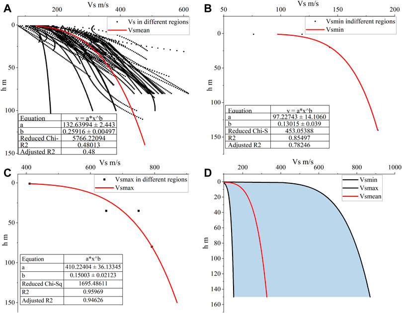
FIGURE 1. Fitting the empirical relationship between Vs and its burial depth in different regions.

2.3 Generating dataset

For a single site velocity structure, the Vs under each burial depth is randomly generated from a truncated normal distribution with $V_{smean}$ as the mean, and $V_{smin}$ and $V_{smax}$ are used as the upper and lower bounds. The layer thickness is a random value within [1, 30] m. When Vs is more than 800 m/s, the number of site layers will not continue to increase. Compared with the layer thickness and Vs, the compression wave velocity and density have less influence on the dispersion curve (Donoho, 1995). The compression wave velocity of each layer is set as twice Vs, and the density is set at 1.85 $g/{cm}^3$. This study generates 10,000 random layer site structures as input and uses the R/T method to calculate the dispersion curve as output. The dataset is divided into a training set and a validation set at a ratio of 4:1. The validation set does not participate in the training of the DL model.

To verify the velocity distribution at different depths, the velocity space at a depth of every meter is divided into 100 cells at 8 m/s intervals. The probability density of each Vs cell is calculated by the percentage of sites in the total dataset. Figure 2 shows the distribution probability of shear velocity occurring at a depth of every meter in 10,000 site samples. Overall, Vs increases with burial depth, and there are two light-colored areas on the left and right. This indicates that the incremental sites make up the majority of the dataset, and a small number of sites have soft or hard interlayers. The estimated area is covered, indicating that the site velocity structure generated with a truncated normal distribution is representative and encompasses all the regions’ sites.

FIGURE 2

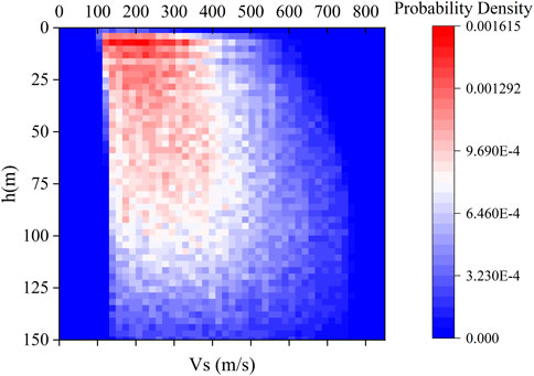
FIGURE 2. Velocity probability density map.

Figure 3 shows the violin plot of the VR dispersion curve corresponding to the random layer site dataset. In the violin plot, the different colors of the violin represent the velocity distribution at different frequencies, and the width of the violin shows the data distribution at different velocities. The wider the violin at the phase velocity is, the more sites with that velocity are in the dataset. The distribution of the violin plot at each frequency is roughly a single peak, and the data distribution is relatively concentrated. The violin shapes at the 1.6 Hz, 2.8 Hz, and 4 Hz frequencies are roughly similar to those at other frequencies. However, more discrete values indicate that the VR value changes significantly in this range, and the dispersion curve is prone to local fluctuation, which requires attention for the frequency range. The local fluctuation in the dispersion curve reflects a soft or hard interlayer. As a result, the frequency distribution of the dispersion curve is reselected. Within 0–1 Hz, the frequency step is set at .2 Hz; within 1–20 Hz, the frequency step is set at .0077 in logarithmic coordinates.

FIGURE 3

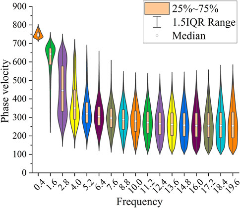
FIGURE 3. Phase velocity dispersion point violin plot.

3 Methods

Constructing a dispersion curve from the site velocity structure is a regression task in deep learning. The commonly used DL models include DNN, CNN, and LSTM. The fully connected dense network is chosen as the main body and is usually called DNN (Bishop, 1995; Nabian and Meidani, 2018). It has a simple architecture and fast learning features. As shown in Figure 4, this paper proposes a network architecture called DNN-BO. The DNN builds the mapping relationship between the site velocity structure and the dispersion curve. Bayesian optimization (BO) is used to automatically select DNN hyperparameters, such as the number of hidden layers, the number of neurons, and the activation function. A complete DNN architecture includes an input layer, some hidden layers, and an output layer. Before inputting the data, the random layer sites sample through the equivalent shear velocity calculation method to make their features correspond one-to-one with the input neurons. The dataset is normalized and input into the network. In the hidden layer, the site velocity structure features are extracted through the neurons connected in pairs. BO updates the DNN architecture based on the cross-validation method objective function minimization. The search strategy outputs the optimal network architecture until the stop condition or iteration count is reached. Finally, the stability, generalization, and efficiency of the rapid method are verified by the validation set.

FIGURE 4

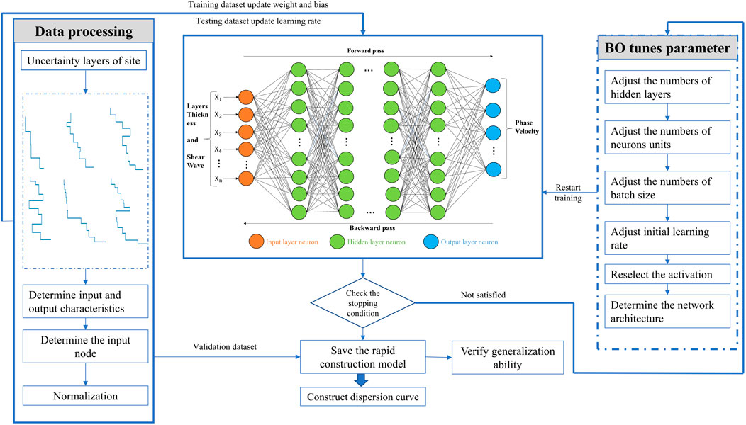
FIGURE 4. Model building flow chart.

3.1 Data processing

In the dataset, the number of site layers and layer thicknesses vary over a wide range. It is better to set a constant node size for the DL model. Therefore, the site layers are converted by the equivalent shear wave velocity method to meet the size of the DNN nodes. As a consequence, the equivalent shear wave velocity method is adopted (Eqs 4–6) to make Vs and the layer thickness correspond to the number of input nodes. In this way, the total number of site layers is standardized at 20. When the dataset contains more than 20 site layers, we prioritize searching for two adjacent layers with a minimum Vs difference. Then, the equivalent shear velocity method is used to calculate the Vs of the original two adjacent layers, and the sum of the two layer thicknesses is used to replace the original thickness. The aforementioned steps are repeated until the dataset contains 20 site layers. When the dataset has fewer than 20 site layers, we search for the thickest layer and divide it into two layers. After the division, the Vs of each layer remains unchanged, and the layer thickness is half the original. The aforementioned process is repeated until the dataset contains 20 site layers.

$t=\sum \frac{v_{si}}{d_i},(4)$

$d=\sum d_i,(5)$

$v_{se}=d/t,(6)$

where $v_{si}$ represents the shear wave velocity of the ith layer, $d_i$ represents the thickness of the ith layer, $v_{se}$ represents the equivalent shear wave velocity, d represents the calculation depth, and t is the sum of the transit times of the shear wave velocity in each layer.

Vs is nearly 100 times larger than the layer thickness. If the original site data are directly input into the neural network, this underestimates the weight of the layer thickness and may lead to premature neural network saturation. Therefore, the max–min normalization method is adopted to normalize the dataset into [0, 1].

$x_i=\frac{X_i-X_{\mathit{min}}}{X_{\mathit{max}}-X_{\mathit{min}}},(7)$

where $X_i$ represents the eigenvalue of the column, $X_{\mathit{min}}$ and $X_{\mathit{max}}$ represent the maximum and minimum values of the eigenvalue of the column, respectively, and $x_i$ represents the normalized eigenvalue.

The well-trained DL model output dispersion curve value is still in the normalized scope and needs to be returned to the original scope. The denormalization formula is shown in Eq. 8:

$\stackrel{\sim }{y}=\dot{y}*\left(y_{\mathit{max}}-y_{\mathit{min}}\right)+y_{\mathit{min}},(8)$

where $\dot{y}$ represents the DL model output value, $y_{\mathit{max}}$ and $y_{\mathit{min}}$ represent the maximum and minimum values of the original data, respectively, and $\stackrel{\sim }{y}$ represents the denormalized value.

3.2 Tuning the DNN hyperparameters using Bayesian optimization algorithms

The DL model itself contains many parameters that need to be determined manually. These parameters are collectively referred to as hyperparameters. The hyperparameters determine the complexity and computational accuracy of the model. There are many types and wide ranges of hyperparameters in the DL models. It is challenging to manually find the most suitable hyperparameter combination for the dataset. At present, hyperparameter optimization mainly depends on the mathematical understanding of the algorithm, empirical judgment, and trial and error (Chauhan and Dhingra, 2012; Assi et al., 2018; Itano et al., 2018; Feurer et al., 2019). However, these empirical methods have a high chance of missing the optimal hyperparameter combination to match the dataset and building a bloated network structure that requires too many computing resources. To find a lightweight and high-precision DL model to construct the dispersion curve, we set DNN as the main body and use the Bayesian optimization algorithm to automatically adjust the hyperparameters, including the number of neurons, number of hidden layers, activation function, learning rate, and training batch size. BO is suitable for multidimensional, high-cost valuation problems and has been widely used in maximum likelihood hyperparameter optimization (Feurer et al., 2019). In the geotechnical engineering and seismic engineering fields, it has been successfully applied for tunnel-boring machine performance prediction (Zhou et al., 2021), slope sensitivity analysis (Sameen et al., 2020) and non-destructive testing (Liang, 2019).

The BO algorithm is based on the evolutionary algorithm combined with the Bayesian network probability model. It contains two primary functions: the surrogate model and the acquisition function (Frazier, 2018). The surrogate model function fits the currently observed points to the objective function and obtains the similarity distribution between the surrogate model and the actual model. The acquisition function is used to select the next evaluated point with the least similarity in the distribution. Both the acquisition function and the surrogate function accelerate the convergence process (Snoek et al., 2015). The main idea of BO is to update the surrogate model by continuously adding new sample points through the acquisition function without knowing the internal structure and mathematical properties of the optimization objective function. It is not until the surrogate model is the same as the actual model or the iteration count is exhausted that the BO outputs the optimal surrogate model. This study uses a Gaussian process (GP) surrogate model that uses the mean and variance to determine the next estimated point. GP has an infinite-dimensional normal distribution extension on an infinite-dimensional random process and can consider multiple hyperparameter optimizations simultaneously (Frazier, 2018).

Figure 5 shows the BO automatic tuning DNN steps. First, the BO initial parameters are set, which includes setting the mean of the k training loss functions as the objective function, setting the GP as the surrogate model, and setting its mean and variance as the acquisition functions. Then, BO randomly selects five DNN hyperparameter combinations to initialize the surrogate model. In each iteration, the next hyperparameter combination evaluation point is determined by the minimum acquisition function similarity. The surrogate model is updated on the objective function value. When the iteration counts are exhausted, the optimization strategy outputs the optimal DNN architecture.

FIGURE 5

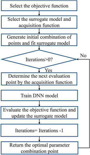
FIGURE 5. Flow chart of Bayesian optimization tuning of the DNN hyperparameters.

Fivefold cross-validation is adopted to avoid overfitting and underfitting situations that significantly influence the stability of the deep learning-based dispersion curve construction (Wong, 2015). Figure 6 shows that the original training set is randomly divided into five equal-sized parts. One part is selected as the test set, and the other four are the training set. The objective function is the mean of the five training loss functions. The cross-validation method makes full use of every sample in the dataset. Each evaluated model will be trained five times in the BO optimization process. In this way, the generalization ability of the rapid method is reinforced.

FIGURE 6

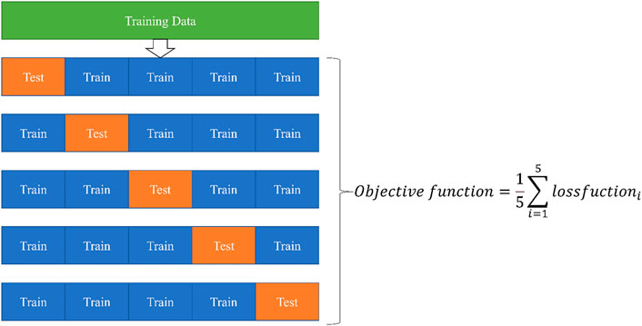
FIGURE 6. Five-fold cross-validation.

The optimization space is closely related to the training cost and the calculational precision. A broad optimization space signifies a more comprehensive hyperparameter combination with higher accuracy and computational costs. A narrow optimization space may miss the optimal DNN architectures. It is expensive to set up an optimization space that includes all the hyperparameter combinations. Referring to deep learning-based surface wave exploration research (Alyousuf et al., 2018; Zhang et al., 2020; Aleardi and Stucchi, 2021; Dai et al., 2021; Fu et al., 2021; Luo et al., 2022), this study sets up four hidden layer blocks. The layers of each hidden layer block are between (0, 2), and the neurons are between (16, 256). The activation function is chosen among the commonly used nonlinear activation functions (“relu,” “elu,” “selu,” “gelu,” “tanh,” and “swish”).

The learning rate is one of the essential hyperparameters in deep learning and is used in training to update the weights and biases of the neurons and to control the loss function change rate (Werbos, 1988). When the learning rate is too high, the loss function changes rapidly as the training progresses, and the convergence speed is fast; however, it may jump back and forth near the optimal solution. In contrast, if the learning rate is too low, the loss function changes very slowly, and the convergence time is too long. The training result may fall into a locally optimal solution. We set the initial learning rate to (.00001, .01) and adopt an adaptive learning rate algorithm. If the loss function remains unchanged every three epochs, the learning rate will become half of the previous one.

The training epochs and batch size determine whether the DNN has fully learned the relationship between the site structure and the dispersion curve (Prechelt et al., 2012; Alwosheel et al., 2018). Insufficient training epochs and a large batch size may lead to an underfitting situation. Therefore, the epochs are set to 100, and the batch size is set to (4, 128).

4 Result

In this section, the DNN-BO model is trained with the random layer site dataset and outputs the optimal DNN architecture. The accuracy and efficiency of the rapid method are verified through the R/T method’s calculation result. The analysis is conducted through a Lenovo R7000P 2020 laptop (R7-4800H CPU, mobile 2060 6GB GPU, and 16GB 3200 Hz DDR4 memory).

4.1 The optimal network architecture

The DNN neurons in the input layer depend on the input data size, as does the output layer. After data processing, there are 39 neurons in the input layer, the VR values are used as the output, and there are 50 neurons in the output layer. This study selects the mean square error (MSE) as the loss function and Adam (Kingma and Ba, 2014) as the optimizer. Figure 7A shows that after 100 iterations, BO can quickly find the DNN architecture most suitable for constructing the dispersion curve. As seen from Table 1, the optimal DNN is a three-hidden-layers simple architecture, in which the hidden layer neurons are 93, 128, and 243, respectively, and “gelu” is set as the activation function. Figure 7B shows that the optimized DNN architecture is not underfitted or overfitted during training and achieves a good convergence state on both the training and validation sets.

FIGURE 7

FIGURE 7. Iterative convergence of the objective function and loss function.

TABLE 1

TABLE 1. DNN hyperparameters search space and the optimal parameters.

4.2 DNN model evaluation

This study sets the mean square error (MSE), mean absolute error (MAE), mean absolute percent error (MAPE), and coefficient of determination ($R^2$) as the overall accuracy evaluation criteria and adopts the ratio of the predicted VR value with the true VR value at each frequency as the local evaluation criterion. The smaller the MSE, MAE, and MAPE values are, the better the calculation effect of the model. $R^2$ represents the degree of correlation between the predicted value and the true value of the target variable. The closer the value of $R^2$ is to 1, the better the degree of correlation. The calculation formulas are as follows:

$MSE=\frac{1}{n}\sum {\left(Y_i-{\stackrel{\sim }{Y}}_i\right)}^2,(9)$

$MAE=\frac{1}{n}\sum \left|Y_i-\overline{Y}\right|,(10)$

$MAPE=\frac{1}{n}\sum \left(\frac{\left|Y_i-{\stackrel{\sim }{Y}}_i\right|}{Y_i}\right)*100\%,(11)$

$R^2=1-\frac{{{\displaystyle \sum }_{i=1}^N\left(Y_i-{\stackrel{\sim }{Y}}_i\right)}^2}{{{\displaystyle \sum }_{i=1}^N\left(Y_i-\overline{Y}\right)}^2},(12)$

where $Y_i$ represents the VR value calculated by the R/T method. ${\stackrel{\sim }{Y}}_i$ represents the VR value calculated by the rapid method. $\overline{Y}$ represents the average VR of the dispersion curve calculated by the R/T method.

The data in Table 2 indicate whether the $R^2$ is more than .97, the MAE value is less than 10, and the MAPE is less than 3.5% in the training set or the validation set. These results suggest that the rapid method is highly correlated with the R/T method and has comparable calculation accuracy.

TABLE 2

TABLE 2. Evaluation standard.

Figure 8 shows the rapid method results and the ratio curves of 12 randomly selected dispersion curves. Figures 8A–D represent relatively smooth dispersion curves, and Figures 8E–H represent dispersion curves with local small-amplitude fluctuations. Their ratio curves between the predicted and true values are almost a line, with only slight fluctuations between 2.5 and 5 Hz. The results show that the calculation accuracy of the rapid method is nearly the same as that of the R/T method on the dispersion curve, with smooth or small local fluctuations. Figures 8I–L represent dispersion curves with strong local fluctuations. There are two positions with local fluctuations. In contrast to the first local fluctuation position, the number of frequency points at the second location is relatively sparse, leading to some deviations in the local change at the high frequency.

FIGURE 8

FIGURE 8. Phase velocity dispersion curve prediction and ratio curve.

The trend in Figure 9 shows that the time spent constructing the dispersion curve by the R/T method increases linearly with the increase in site layers, and the time spent by the rapid method changes little, if at all. When calculating the site model with 10, 50, and 100 layers, the R/T method takes 15.77 s, 49.45 s, and 88.18 s, respectively. The rapid method takes less than .05 s, and its computational cost only slightly increases with the increase in site layers. The rapid method and R/T method are used to calculate all the samples in the validation set and take 59 s and 23,473.8 s, respectively. The aforementioned analysis and time consumption ratio curve show that the rapid method improves the computational efficiency by at least 400 times while ensuring the same accuracy.

FIGURE 9

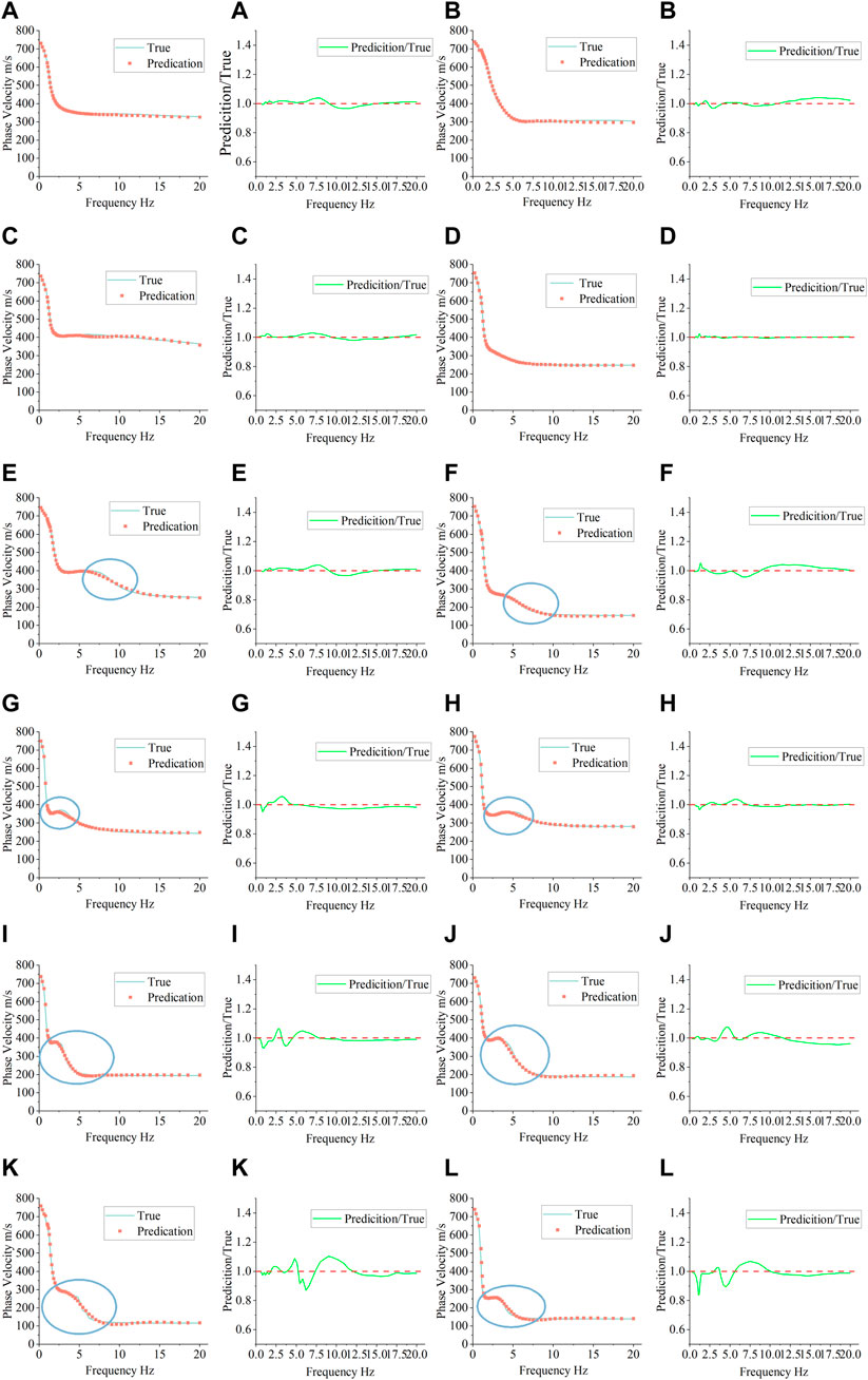
FIGURE 9. Calculating time and time consumption ratio.

5 Discussion

Compared with the conventional forward method, the rapid method has high computational efficiency and the same accuracy, but it also has some limitations.

5.1 Influence of soft or hard interlayer

The conventional forward modeling method can directly calculate the site of the arbitrary velocity structure; however, the rapid method is affected by the size and distribution of the dataset for training the model. In the validation set, the mean ratio difference (MRD) of all 2000 site samples was calculated (Eq. 14). Approximately 2% of the site samples had an MRD greater than 5%. Figure 10 shows the dispersion curves and velocity structures of the three site samples with the largest MRD. There is a large soft or hard interlayer in the shallow layer, and the overall velocity structure fluctuates back and forth. That situation makes a small part of the dispersion curves fluctuate locally at high frequencies. Both sites with a back-and-forth fluctuation velocity structure and high-frequency dispersion curve frequency points are very sparse in the dataset, which leads to insufficient DNN learning for those site characteristics. More research is required to balance the back-and-forth fluctuation site ratio and to maintain the main site characteristics in the dataset.

$MRD=\left({\displaystyle \sum }_{i=1}^n\left|\frac{y\_true}{y\_pred}\right|/n-1\right)*100\%,(13)$

where y_true and y_pred represent the VR calculated by the R/T method and the VR calculated by the rapid method, respectively.

FIGURE 10

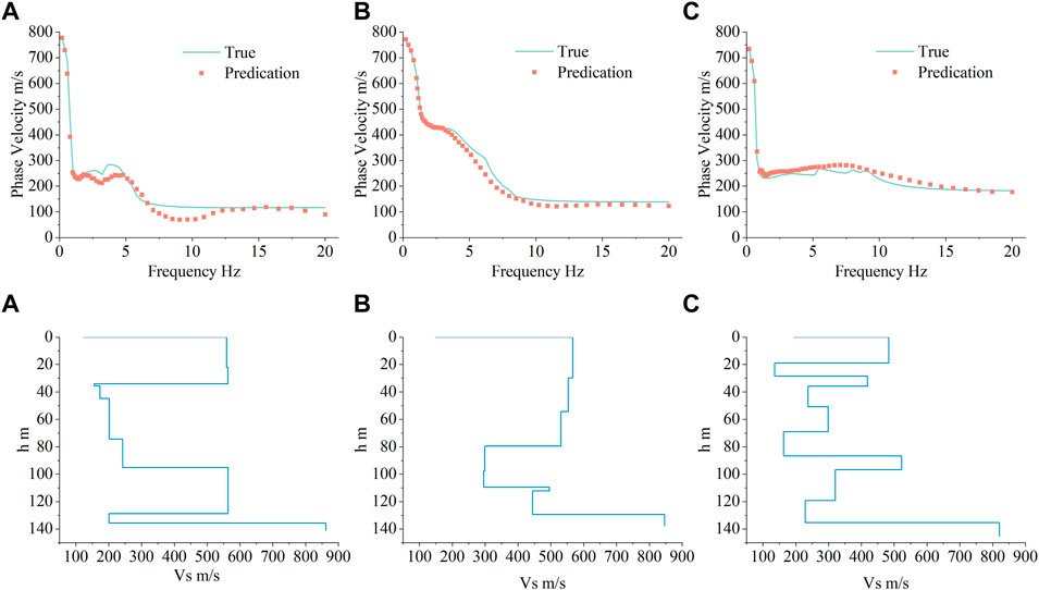
FIGURE 10. Phase velocity dispersion curve prediction graph and velocity structure graph.

5.2 Selection of frequency points

The frequency points of the rapid method output are fixed. However, in practical engineering, the frequency points are generally equidistant, and the number of required frequency points is determined by the site complex. Therefore, we propose a linear interpolation method to calculate the VR at a specific frequency. Assuming that the VR of point x is needed, the rapid method can be used to calculate the left adjacent point x₀, VR f (x₀), right adjacent point x₁, and VR f (x₁). Moreover, it is substituted into Formula (14) to calculate the VR of this frequency point.

$f\left(x\right)=\frac{x-x_1}{x_0-x_1}*f\left(x_0\right)+\frac{x-x_0}{x_1-x_0}*f\left(x_1\right).(14)$

As shown in Figure 11, the solid green line and the red dots represent the .4 Hz frequency step dispersion curve calculated by the interpolation and R/T methods, respectively. When using the rapid method to construct the dispersion curve with equal frequency steps, the interpolation process may ignore the local fluctuation of the high-frequency band because the high-frequency dispersion points are relatively sparse. Some deviations are applied to the population-based inversion algorithm. Considering that there are relatively few of these kinds of sites in the earth’s sedimentary system, we will seek deep learning or data-driven methods to solve this problem in future studies, and the R/T method will be chosen when there is the rare need for high precision. For population-based inversion, our rapid method can be effectively applied to construct the dispersion curve of most sites. The R/T method may be further applied to sites with very thin soft/hard interlayers to improve the inversion accuracy.

FIGURE 11

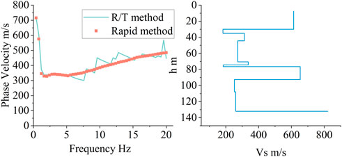
FIGURE 11. Interpolated phase velocity dispersion curve graph and its velocity structure graph.

5.3 Influence of the number of datasets

Figure 12A shows the computational performance of the rapid method for nine datasets of different sizes. With the increase in samples, the box size gradually decreases, the 90% confidence interval gradually shrinks, and the distribution of the prediction results is gradually concentrated. Figure 12B shows the variation in $R^2$ and MAE with the number of samples for the same nine datasets. As the number of samples in the dataset increases, $R^2$ rises quickly, and the MAE falls quickly. When the sample size of the dataset is more than 7,000, the change trend slows down significantly. This means that each DNN architecture needs only 7,000 samples, and the model is basically in a convergence state. Therefore, when rebuilding the rapid construction method of other frequency bands, a dataset size set at 7,000 samples is sufficient.

FIGURE 12

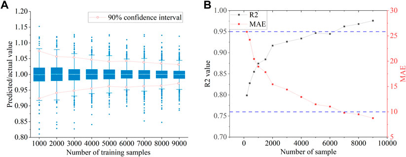
FIGURE 12. Effect of dataset size: (A) boxplot and 90% confidence interval; (B) R² and MAE with increasing sample size.

6 Conclusion

This paper proposes a deep learning-based method for rapidly constructing 1D dispersion curves. The method consists of two essential parts: building a reasonable random site dataset and building a high-precision, lightweight network architecture. For the dataset, we distill a general empirical relationship between Vs and the burial depth through Vs–h empirical relationships in nine different regions of China. Based on this, a technique to generate a random layer site dataset that ensures the diversity and representativity of the dataset and improves the generalization and applicability of the rapid method is proposed. To build the network architecture, the Bayesian optimization algorithm is used to automatically find the optimal DNN architectures, which include three hidden layers, and “gelu” is applied as the activation function. This network architecture is well suited for learning the relationship between the site velocity structure and the dispersion curve. Finally, a validation set is used to verify the rapid method’s accuracy, stability, generalization, and computational efficiency. Based on the analysis of the results, the following conclusions can be drawn:

1) In both the training and validation sets, $R^2$ is more than .97, MAE is less than 10, and MAPE is less than 3.5%. The evaluation result from the aforementioned analysis indicates that the rapid method has comparable accuracy with the R/T method in calculating the dispersion curve.

2) It is difficult for the rapid method to identify the local fluctuations in the high-frequency band of the dispersion curve. In the dataset, 2% of the site samples have an MRD greater than 5%, and in most of those sites, Vs fluctuates back and forth, which causes a local fluctuation in the high-frequency dispersion curve. An implication of this is the possibility that the rapid method is poor at constructing dispersion curves where the site velocity structure fluctuates.

3) Once the training is completed, the rapid method improves the computational efficiency by at least 400 times while ensuring the same accuracy. There is almost no increase in computation expense with an increase in site layers. This method uses a trained neural network to replace the complex calculation processes of many matrix multiplications, transfer matrix iterations and recursive approximations in the matrix method. The computational cost of multiple iterative forward modeling is greatly reduced, especially when the population-based inversion algorithm searches for multilayer site structures.

4) The number of samples impacts the prediction performance of the rapid method. A dataset of 7,000 samples is sufficient to obtain a stable model.

Data availability statement

The original contributions presented in the study are included in the article/Supplementary Material; further inquiries can be directed to the corresponding author.

Author contributions

DC handled most of the work of the article. LS provided the main idea of the article and was the main contributor to guide the revision of the article. KG determined the statistical Vs–h empirical relationship and provided some suggestions for the article.

Funding

This work was supported by the National Natural Science Foundation of China (Grant No. 51978635).

Acknowledgments

The authors thank the editor and reviewers for their valuable comments on this paper and the Institute of Engineering Mechanics, China Earthquake Administration, for supporting this research. All programs have been created using the Python and Tensorflow computational frameworks.

Conflict of interest

The authors declare that the research was conducted in the absence of any commercial or financial relationships that could be construed as a potential conflict of interest.

Publisher’s note

All claims expressed in this article are solely those of the authors and do not necessarily represent those of their affiliated organizations, or those of the publisher, the editors, and the reviewers. Any product that may be evaluated in this article, or claim that may be made by its manufacturer, is not guaranteed or endorsed by the publisher.

Supplementary material

The Supplementary Material for this article can be found online at: https://www.frontiersin.org/articles/10.3389/feart.2022.1084414/full#supplementary-material

References

Abo-Zena, A. (1979). Dispersion function computations for unlimited frequency values. Geophys. J. Int. 58 (1), 91–105. doi:10.1111/j.1365-246X.1979.tb01011.x

CrossRef Full Text | Google Scholar

Aleardi, M., and Stucchi, E. (2021). A hybrid residual neural network–Monte Carlo approach to invert surface wave dispersion data. Near Surf. Geophys. 19 (4), 397–414. doi:10.1002/nsg.12163

CrossRef Full Text | Google Scholar

Alwosheel, A., van Cranenburgh, S., and Chorus, C. G. (2018). Is your dataset big enough? Sample size requirements when using artificial neural networks for discrete choice analysis. J. choice Model. 28, 167–182. doi:10.1016/j.jocm.2018.07.002

CrossRef Full Text | Google Scholar

Alyousuf, T., Colombo, D., Rovetta, D., and Sandoval-Curiel, E. (2018). “Near-surface velocity analysis for single-sensor data: An integrated workflow using surface waves, AI, and structure-regularized inversion,” in SEG technical program expanded abstracts 2018 SEG technical program expanded abstracts (Tulsa, Oklahoma: Society of Exploration Geophysicists), 2342–2346. doi:10.1190/segam2018-2994696.1

CrossRef Full Text | Google Scholar

Assi, K. J., Nahiduzzaman, K. M., Ratrout, N. T., and Aldosary, A. S. (2018). Mode choice behavior of high school goers: Evaluating logistic regression and MLP neural networks. Case Stud. Transp. policy 6 (2), 225–230. doi:10.1016/j.cstp.2018.04.006

CrossRef Full Text | Google Scholar

Aung, A. M., and Leong, E. C. (2010). Discussion of “near-field effects on array-based surface wave methods with active sources” by S. Yoon and G. J. Rix. J. Geotechnical Geoenvironmental Eng. 136, 773–775. doi:10.1061/(ASCE)GT.1943-5606.0000131

CrossRef Full Text | Google Scholar

Bishop, C. M. (1995). Neural networks for pattern recognition. Clarendon Press. New York, NY: Oxford University Press.

Google Scholar

Boore, D. M. (1972). Finite difference methods for seismic wave propagation in heterogeneous materials. Methods Comput. Phys. 11, 1–37. doi:10.1016/B978-0-12-460811-5.50006-4

CrossRef Full Text | Google Scholar

Chauhan, S., and Dhingra, S. (2012). Pattern recognition system using MLP neural networks. Pattern Recognit. 4 (9), 990–993. doi:10.9790/3021-0205990993

CrossRef Full Text | Google Scholar

Chen, X. (1993). A systematic and efficient method of computing normal modes for multilayered half-space. Geophys. J. Int. 115 (2), 391–409. doi:10.1111/j.1365-246X.1993.tb01194.x

CrossRef Full Text | Google Scholar

Dai, T., Xia, J., Ning, L., Xi, C., Liu, Y., and Xing, H. (2021). Deep learning for extracting dispersion curves. Surv. Geophys. 42 (1), 69–95. doi:10.1007/s10712-020-09615-3

CrossRef Full Text | Google Scholar

Donoho, D. L. (1995). De-noising by soft-thresholding. IEEE Trans. Inf. theory 41 (3), 613–627. doi:10.1109/18.382009

CrossRef Full Text | Google Scholar

Faccioli, E., Maggio, F., Quarteroni, A., and Taghan, A. (1996). Spectral-domain decomposition methods for the solution of acoustic and elastic wave equations. Geophysics 61 (4), 1160–1174.

CrossRef Full Text | Google Scholar

Fan, Y. H., Liu, J. Q., and Xiao, B. X. (2002). Fast vector-transfer algorithm for computation of Rayleigh wave dispersion curves. J. Hunan Univ. 29 (5), 25–30. doi:10.1190/1.1444036

CrossRef Full Text | Google Scholar

Feurer, M., Klein, A., Eggensperger, K., Springenberg, J. T., Blum, M., and Hutter, F. (2019). Auto-sklearn: Efficient and robust automated machine learning, part of the Springer series on challenges in machine learning book series (SSCML). Berlin, Germany: Spinger. doi:10.1007/978-3-030-05318-5_6

CrossRef Full Text | Google Scholar

Frazier, P. I. (2018). Bayesian optimization. Inf. TutORials Operations Res. 2018, 255–278. doi:10.1287/educ.2018.0188

CrossRef Full Text | Google Scholar

Fu, L., Pan, L., Ma, Q., Dong, S., and Chen, X. (2021). Retrieving S-wave velocity from surface wave multimode dispersion curves with DispINet. J. Appl. Geophys. 193, 104430. doi:10.1016/j.jappgeo.2021.104430

CrossRef Full Text | Google Scholar

Guo, Q., Ba, J., and Luo, C. (2021). Prestack seismic inversion with data-driven MRF-based regularization. IEEE Trans. Geoscience Remote Sens. 59, 7122–7136. doi:10.1109/TGRS.2020.3019715

CrossRef Full Text | Google Scholar

Haskell, N. A. (1953). The dispersion of surface waves on multilayered media. Bull. Seismol. Soc. Am. 43 (1), 17–34. doi:10.1785/BSSA0430010017

CrossRef Full Text | Google Scholar

He, Y. F., and Chen, C. F. (2006). Normal mode computation by the generalized reflection transmission coefficient method in planar layered half space. Chin. J. Geophys. 49 (4), 1074–1081. doi:10.3321/j.issn:0001-5733.2006.04.020

CrossRef Full Text | Google Scholar

Hisada, Y. (1994). An efficient method for computing Green's functions for a layered half-space with sources and receivers at close depths. Bull. Seismol. Soc. Am. 84 (5), 1456–1472. doi:10.1785/BSSA0840051456

CrossRef Full Text | Google Scholar

Hisada, Y. (1995). An efficient method for computing Green's functions for a layered half-space with sources and receivers at close depths (Part 2). Bull. Seismol. Soc. Am. 85 (4), 1080–1093. doi:10.1785/BSSA0850041080

CrossRef Full Text | Google Scholar

Itano, F., de Sousa, M. A. D. A., and Del-Moral-Hernandez, E. (2018). “Extending MLP ANN hyper-parameters optimization by using genetic algorithm,” in 2018 International joint conference on neural networks (IJCNN), Rio de Janeiro, Brazil, 08-13 July 2018 (IEEE), 1–8. doi:10.1109/IJCNN.2018.8489520

CrossRef Full Text | Google Scholar

Jo, S., Jeong, H., Min, B., Park, C., Kim, Y., Kwon, S., et al. (2022). Efficient deep-learning-based history matching for fluvial channel reservoirs. J. Petroleum Sci. Eng. 208, 109247. doi:10.1016/j.petrol.2021.109247

CrossRef Full Text | Google Scholar

Kennett, B. L. N., and Clarke, T. J. (1983). Seismic waves in a stratified half-space—IV: P—SV wave decoupling and surface wave dispersion. Geophys. J. Int. 72 (3), 633–645. doi:10.1111/j.1365-246X.1983.tb02824.x

CrossRef Full Text | Google Scholar

Kennett, B. L. N., and Kerry, N. J. (1979). Seismic waves in a stratified half space. Geophys. J. Int. 57 (3), 557–583. doi:10.1111/j.1365-246X.1979.tb06779.x

CrossRef Full Text | Google Scholar

Kennett, B. L. N. (1974). Reflections, rays, and reverberations. Bull. Seismol. Soc. Am. 64 (6), 1685–1696. doi:10.1785/BSSA0640061685

CrossRef Full Text | Google Scholar

Kingma, D. P., and Ba, J. (2014). Adam: A method for stochastic optimization. arXiv preprint arXiv:1412.6980. doi:10.48550/arXiv.1412.6980

CrossRef Full Text | Google Scholar

Komatitsch, D., and Vilotte, J. P. (1998). The spectral element method: An efficient tool to simulate the seismic response of 2D and 3D geological structures. Bull. Seismol. Soc. Am. 88 (2), 368–392. doi:10.1785/BSSA0880020368

CrossRef Full Text | Google Scholar

Lei, Y., Shen, H., Li, X., Wang, X., and Li, Q. (2019). Inversion of Rayleigh wave dispersion curves via adaptive GA and nested DLS. Geophys. J. Int. 218 (1), 547–559. doi:10.1093/gji/ggz171

CrossRef Full Text | Google Scholar

Liang, X. (2019). Image-based post-disaster inspection of reinforced concrete bridge systems using deep learning with Bayesian optimization. Computer-Aided Civ. Infrastructure Eng. 34 (5), 415–430. doi:10.1111/mice.12425

CrossRef Full Text | Google Scholar

Lu, Y., Peng, S., Du, W., Zhang, X., Ma, Z., and Lin, P. (2016). Rayleigh wave inversion using heat-bath simulated annealing algorithm. J. Appl. Geophys. 134, 267–280. doi:10.1016/j.jappgeo.2016.09.008

CrossRef Full Text | Google Scholar

Luco, J. E., and Apsel, R. J. (1983). On the Green's functions for a layered half-space. Part I. Bull. Seismol. Soc. Am. 73 (4), 909–929. doi:10.1785/BSSA0730040909

CrossRef Full Text | Google Scholar

Luo, C., Ba, J., and Carcione, J. M. (2022a). A hierarchical prestack seismic inversion scheme for VTI media based on the exact reflection coefficient. IEEE Trans. Geoscience Remote Sens. 60, 1–16. doi:10.1109/TGRS.2021.3140133

CrossRef Full Text | Google Scholar

Luo, Y., Huang, Y., Yang, Y., Zhao, K., Yang, X., and Xu, H. (2022b). Constructing shear velocity models from surface wave dispersion curves using deep learning. J. Appl. Geophys. 196, 104524. doi:10.1016/j.jappgeo.2021.104524

CrossRef Full Text | Google Scholar

Manolis, G. D., and Beskos, D. E. (1988). Boundary element methods in elastodynamics. New York, NY: Taylor & Francis. doi:10.1115/1.3173761

CrossRef Full Text | Google Scholar

Nabian, M. A., and Meidani, H. (2018). Deep learning for accelerated seismic reliability analysis of transportation networks. Computer-Aided Civ. Infrastructure Eng. 33, 443–458. doi:10.1111/mice.12359

CrossRef Full Text | Google Scholar

Pan, L., Yuan, S., and Chen, X. (2022). Modified generalized R/T coefficient method for surface-wave dispersion-curve calculation in elastic and viscoelastic media. Bull. Seismol. Soc. Am. 112, 2280–2296. doi:10.1785/0120210294

CrossRef Full Text | Google Scholar

Picozzi, M., and Albarello, D. (2007). Combining genetic and linearized algorithms for a two-step joint inversion of Rayleigh wave dispersion and H/V spectral ratio curves. Geophys. J. Int. 169 (1), 189–200. doi:10.1111/j.1365-246X.2006.03282.x

CrossRef Full Text | Google Scholar

Poormirzaee, R., and Fister, I. (2021). Model-based inversion of Rayleigh wave dispersion curves via linear and nonlinear methods. Pure Appl. Geophys. 178 (2), 341–358. doi:10.1007/s00024-021-02665-7

CrossRef Full Text | Google Scholar

Poormirzaee, R. (2016). S-wave velocity profiling from refraction microtremor Rayleigh wave dispersion curves via PSO inversion algorithm. Arabian J. Geosciences 9 (16), 673–710. doi:10.1007/s12517-016-2701-6

CrossRef Full Text | Google Scholar

Prechelt, L. (2012). “Neural networks: Tricks of the trade,” in Early stopping—but when? Editors G. Montavon, G. B. Orr, and K. R. Müller second edition (Berlin, Heidelberg: Springer Berlin Heidelberg), 53–67. doi:10.1007/978-3-642-35289-8_5

CrossRef Full Text | Google Scholar

Sameen, M. I., Pradhan, B., and Lee, S. (2020). Application of convolutional neural networks featuring Bayesian optimization for landslide susceptibility assessment. Catena 186, 104249. doi:10.1016/j.catena.2019.104249

CrossRef Full Text | Google Scholar

Schwab, F. A., and Knopoff, L. (1972). Fast surface wave and free mode computations. Methods Comput. Phys. Adv. Res. Appl. 11, 87–180. doi:10.1016/B978-0-12-460811-5.50008-8

CrossRef Full Text | Google Scholar

Schwab, F., and Knopoff, L. (1970). Surface-wave dispersion computations. Bull. Seismol. Soc. Am. 60 (2), 321–344. doi:10.1785/BSSA0600020321

CrossRef Full Text | Google Scholar

Snoek, J., Rippel, O., Swersky, K., Kiros, R., Satish, N., Sundaram, N., et al. (2015). Scalable bayesian optimization using deep neural networks Proceedings of the 32nd international Conference on machine learning (PMLR), 2171–2180. Available at: https://proceedings.mlr.press/v37/snoek15.html (Accessed October 29, 2022).

Google Scholar

Takeuchi, H., and Saito, M. (1972). Seismic surface waves. Methods Comput. Phys. 11, 217–295. doi:10.1016/B978-0-12-460811-5.50010-6

CrossRef Full Text | Google Scholar

Thomson, W. T. (1950). Transmission of elastic waves through a stratified solid medium. J. Appl. Phys. 21 (2), 89–93. doi:10.1063/1.1699629

CrossRef Full Text | Google Scholar

Tschannen, V., Ghanim, A., and Ettrich, N. (2022). Partial automation of the seismic to well tie with deep learning and Bayesian optimization. Comput. Geosciences 164, 105120. doi:10.1016/j.cageo.2022.105120

CrossRef Full Text | Google Scholar

Wamriew, D., Charara, M., and Pissarenko, D. (2022). Joint event location and velocity model update in real-time for downhole microseismic monitoring: A deep learning approach. Comput. Geosciences 158, 104965. doi:10.1016/j.cageo.2021.104965

CrossRef Full Text | Google Scholar

Werbos, P. J. (1988). Generalization of backpropagation with application to a recurrent gas market model. Neural Netw. 1 (4), 339–356. doi:10.1016/0893-6080(88)90007-X

CrossRef Full Text | Google Scholar

Wong, T. T. (2015). Performance evaluation of classification algorithms by k-fold and leave-one-out cross validation. Pattern Recognit. 48 (9), 2839–2846. doi:10.1016/j.patcog.2015.03.009

CrossRef Full Text | Google Scholar

Zhang, X., Jia, Z., Ross, Z. E., and Clayton, R. W. (2020). Extracting dispersion curves from ambient noise correlations using deep learning. IEEE Trans. Geoscience Remote Sens. 58, 8932–8939. doi:10.1109/TGRS.2020.2992043

CrossRef Full Text | Google Scholar

Zhou, J., Qiu, Y., Zhu, S., Armaghani, D. J., Khandelwal, M., and Mohamad, E. T. (2021). Estimation of the TBM advance rate under hard rock conditions using XGBoost and Bayesian optimization. Undergr. Space 6 (5), 506–515. doi:10.1016/j.undsp.2020.05.008

CrossRef Full Text | Google Scholar