Evaluation of spaceborne GNSS-R based sea surface altimetry using multiple constellation signals

Comparisons between different global navigation satellite system (GNSS) signals and GNSS-reflectometry (GNSS-R) satellite systems can provide valuable suggestions for future development of the GNSS-R instrument and signal processing method. This article evaluates the ocean altimetry performance of multiple GNSS constellation signals using raw intermediate frequency data collected by Cyclone GNSS (CYGNSS) and TechDemoSat-1 (TDS-1) satellites. Data used for the evaluation include observations of GPS L1, Galileo E1, and BDS B1 band signal. The specular point position and the ground-truth bistatic delay are calculated through the HALF method. After ionospheric, tropospheric, and tide corrections, the sea surface height can be retrieved; and then the height is compared with the DTU18 mean sea surface model derived one. Based on the GNSS-R satellite-collected observations, an optimal incoherent integral duration is determined. By making use of the optimal duration, the CYGNSS-based ranging delay estimating accuracy can reach up to 2.38 m, 1.98 m, and 1.91 m for GPS, Galileo and BDS, respectively; and the TDS-1 based one can reach up to 5.46 m and 3.84 m for GPS and Galileo, respectively. The results can provide suggestion on the strategies of multi-constellation observations fusion to improve the altimetry accuracy.

1 Introduction

The ocean covers about 70% of the Earth’s surface, and sea surface height (SSH) is of great importance for research of ocean circulation and global climate change (Levermann et al., 2005; Bindoff et al., 2007). As the main spaceborne-based SSH observing technology, radar altimetry is limited by its sub-satellite observation mode, only resolving mesoscale features larger than 400 km (FU et al., 2010). A new technology is necessary for observing small mesoscale and sub-mesoscale SSH with higher temporal and spatial resolution. The GNSS-R aims to retrieve information of the Earth’s surface through analyzing the signals transmitted by GNSS satellites and the signals reflected from the sea surface. Since the PARIS (passive reflectometry and interferometric system) concept proposed in 1993, GNSS-R has been demonstrated as an effective technique for estimating geophysical parameters such as soil moisture, sea surface wind speed, and SSH (Martín-Neira, 1993; Clarizia et al., 2016, 2019; Clarizia and Ruf, 2016). Compared to the traditional radar altimetry techniques, GNSS-R-based ocean altimetry is a promising technique due to high temporal and spatial resolution. Because of the passive sensing mode and bistatic radar properties, the GNSS-R instrument has a significant advantage in terms of economic cost, power requirement, and monitoring coverage. With improvement of the technology, it would provide more opportunities for retrieving mesoscale SSH information.

Preliminary research about the configuration of bistatic altimeter constellation and the bistatic model of ocean scattering has provided guidelines for receiver design (Martin-Neira et al., 1998; Picardi et al., 1998; Hajj and Zuffada, 2003). Based on the early work, GNSS-R altimetry has been validated by various ground and airborne experiments, which also creates theoretical and experimental foundations for spaceborne-based GNSS-R altimetry (Lowe et al., 2000, 2002; Martin-Neira et al., 2001, 2002; Treuhaft et al., 2001). UK-DMC (disaster monitoring constellation), which is the first satellite equipped with a GNSS-R receiver, was launched in 2003 (Gleason et al., 2005). The satellite had been collecting numerous observations, validating the feasibility of the GNSS-R-based altimetry technique. After that, TDS-1 was launched in July 2014; the GNSS-R receiver carried by the satellite could output the delay-Doppler maps (DDMs) which contain information about the delay and Doppler around a specular point (SP) (Unwin et al., 2016). In recent years, an improved receiver was used on the NASA’s CYGNSS mission for monitoring ocean wind speed (Ruf et al., 2012, 2016). Because of the improvement of the GNSS-R instrument, the signals transmitted by GPS, Galileo, and BDS can also be received and processed by the Delay–Doppler mapping instrument (DDMI). In addition to more observations, a multi-constellation signal can also provide an opportunity to explore the discrepancies in GNSS-R ocean altimetry performance of GNSS signals with a different band and modulation. Thus, strategies of multi-constellation observation fusion can be derived for improving the altimetry accuracy.

In this work, we concentrate on the determination of optimal integration duration and the comparison of code phase altimetry performance of different GNSS constellation and GNSS-R satellite systems. The work could provide a reasonable basis for combining multi-constellation SSH estimations in the future. This article is organized as follows. In the next section, the datasets used in the paper are introduced. Details of the GNSS-R-based altimetry method are described in Section 3. The altimetry performance and the comparison between the different satellite constellations are presented in Section 4. Section 5 concludes this paper.

2 Data

The raw intermediate frequency (IF) data are raw sensor counts, which come from the incoming radio frequency streams, digitized by DDMI. The raw IF data records are downlinked by ground commands to coincide with an overpass of a target area of interest. Therefore, it provides opportunities to explore potential abilities of GNSS-R with the highest resolution in delay and Doppler space for advanced science applications. The raw IF data pre-processed by Institut d’Estudis Espacial de Catalunya (IEEC) and available on IEEC’s GPS Open Loop Differential Real-Time Receiver Data server (IEEC GOLD-RTR) are used in this paper. It consists of a complex waveform (cWF) file and metadata file. In the cWF file, there are raw signal sample streams (30 s–90 s) of direct signals and reflected signals received by zenith antenna and nadir antenna, respectively. The metadata file mainly contains geometric information, such as positioning and timing information of the GNSS-R spacecraft, GNSS constellation, and the incidence angle.

The raw IF data used in the paper were collected by two GNSS-R constellations: TDS-1 and CYGNSS. TDS-1 was intermittently operating in the sun-synchronous orbit with 650-km altitude and inclination of 98.4°; while CYGNSS consists of eight microsatellites in one plane with 520-km altitude and inclination of 35°. Parameters of the GNSS-R instrument used by TDS-1 and the CYGNSS are shown in Table 1. Some parameters have been improved for the CYGNSS; especially, a cavity filter was used for the CYGNSS instead of a dielectric filter, which could result in a lower noise figure and thus lower observing noising and thus higher quality of GNSS observations (Jales, 2015).

TABLE 1

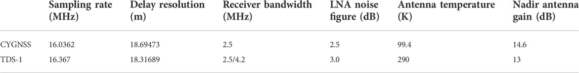
TABLE 1. Configuration of RF front-end onboard CYGNSS/TDS-1.

The datasets used in the paper include TDS-1 raw IF observations collected from September 2014, to March 2019, and CYGNSS raw IF observations collected from September 2017, to September 2022, as shown in Figure 1 and Table 2. It should be noted that CY_GPS, CY_Galileo, and CY_BDS indicate that the CYGNSS collected GPS, Galileo, and BDS signals, respectively; TDS_GPS and TDS_Galileo indicate the TDS-1-collected GPS and Galileo signals, respectively. The satellite tracks are 189, 99, 75, 288, and 58 for these five schemes, respectively. It should be noted that because the TDS-1 mission was terminated in 2019, few BDS observations are recorded by TDS-1 to derive reliable research.

FIGURE 1

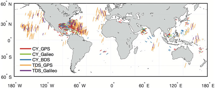
FIGURE 1. Map of specular point ground tracks of the raw IF data used in analysis, with different colors indicating data sources. The number of the tracks is presented in Table 2.

TABLE 2

TABLE 2. Details about data used in the paper.

3 Methodology

3.1 Geometry of spaceborne GNSS-R-based SSH estimation

The geometry of spaceborne GNSS-R based SSH estimation is shown in Figure 2. The signal transmitted by a GNSS satellite (e.g., GPS, Galileo, or BDS satellite) travels approximately 20,000 km to reach the sea surface. Once the signal reaches the sea surface, it would be reflected by the surface into the near-Earth-space and be received by the low-Earth-orbit satellite (e.g., TDS-1 or CYGNSS satellite). In addition, a part of the GNSS satellite transmitted signal would also be received by the low-Earth-orbit (LEO) satellite directly. Compared with the latter, the former travels an additional path length, which is the path delay between the transmitter signal and the reflected signal, and the path delay can be expressed as follows:

${\mathit{\rho }}_{\mathbf{1}}=\mathbf{2}{\mathit{H}}_{\mathbf{1}}\mathit{sin}\mathit{\theta },(1)$

where $\theta$ is the GNSS satellite elevation angle and $H_1$ is height of the LEO satellite relative to the sea surface. Similarly, if the signal transmitted by the GNSS satellite is reflected by a virtual surface (e.g., surface of reference ellipsoid of World Geodetic System 1984, WGS84), the path delay can be written as follows:

${\mathit{\rho }}_{\mathbf{2}}=\mathbf{2}{\mathit{H}}_{\mathbf{2}}\mathit{sin}\mathit{\theta },(2)$

where $H_2$ is the height of the LEO satellite relative to the virtual surface.

FIGURE 2

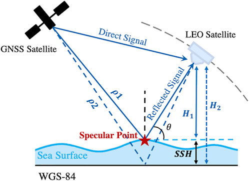
FIGURE 2. Geometry of spaceborne GNSS-R based SSH estimation.

The additional traveling path length of ${\rho }_2$ can be calculated directly based on the 3D position of the GNSS satellite, LEO satellite, and the virtual specular reflection point. If the length of ${\rho }_1$ can be obtained with the LEO satellite received by direct and reflected GNSS signals, then SSH of the reflection points of the sea surface relative to the virtual surface can be obtained by

$\mathit{S}\mathit{S}\mathit{H}={\mathit{H}}_{\mathbf{2}}-{\mathit{H}}_{\mathbf{1}}=\frac{{\mathit{\rho }}_{\mathbf{2}}-{\mathit{\rho }}_{\mathbf{1}}}{\mathbf{2}\mathit{sin}\mathit{\theta }}.(3)$

The description mentioned previously summarizes the geometry principle of the spaceborne GNSS-R based SSH estimation. Obviously, the key of the method is estimation of additional path length of ${\rho }_1$, which is detailed in the following contents.

3.2 SSH retrieval procedure

Figure 3 shows the SSH retrieval procedure using the GNSS-R raw IF data. Because black body load is selected occasionally during the sampling period and TDS-1 operated in high-latitude orbit, data pre-procession is necessary to avoid disturbance of black body observations and sea ice observations. In the meanwhile, for satisfying the data quality requirement, a series of quality control steps should be conducted at first. The quality control contents are listed as follows:

1) Specular points with latitude greater than 55° should be eliminated to avoid coherent measurements from sea ice in TDS-1 datasets.

2) The measurements used for black body calibrations should be removed.

3) The incidence angle should be limited up to 60° and the wind speed be set to be greater than 3 m/s to reduce the coherent components in the reflected signals (Voronovich and Zavorotny, 2018).

4) The signal-to-noise ratio (SNR) at SP is controlled in the scale (–7.0 dB, 10 dB) to ensure that the incoherent component of reflected signals dominate and avoid the impact of direct signal interference.

FIGURE 3

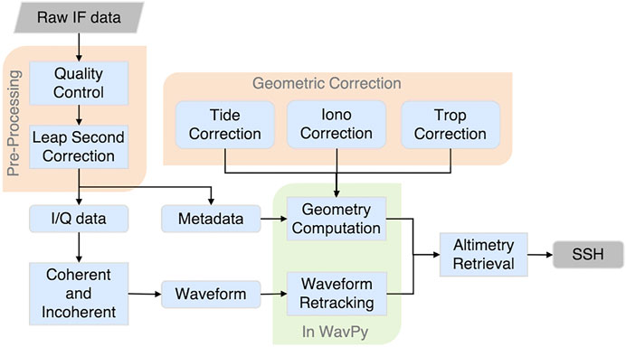
FIGURE 3. SSH retrieval procedure based on raw IF data.

To verify the accuracy of the transmitter orbit provided in raw IF datasets, the precise ephemeris of Wuhan University GNSS Research Center is used to calculate the position of the transmitter at a given time stamp, and an 18-s delay was found which might be due to the negligence of a leap second in the conversion between GPSs and UTCs when metadata were processed on the ground at UTC time stamp. Thus, a leap second correction is needed in computing several time-dependent parameters, such as tide correction and wind speed. The error might reach to ±0.3 mm in 1-s SSH measurements without correction.

After quality control and leap second correction, the IF data can be used to perform coherent and incoherent integration, producing a clear delay waveform to extract the observed path delay. With the geometry relationship, the modeled path delay could be obtained by geometry computation plus various corrections, and then the final SSH measurements are calculated by the altimetry retrieval method presented in the previous section.

3.3 Derivation of delay waveform from raw IF

In the raw IF data processing stage of IEEC-GOLD, the signal streams were integrated coherently at a constant period of 1 ms (Li et al., 2022). Thus, the complex delay waveform provided by the cWF file was with resolution of 1 ms. However, the amplitude of the reflected signals is still weak than that of the direct signals; thus, it is difficult to directly extract useful information from the waveform. Hence, it is necessary to perform coherent integration and incoherent accumulation for enhancing the strength of the useful signals.

3.3.1 Coherent and incoherent integration

The coherent and incoherent integration methods are summarized by Yang et al. (2007). For clarity, the formulae of coherent and incoherent integration are simplified as follows.

The coherent integration is directly superimposing the real and imaginary parts of complex waveforms as follows:

${\mathit{Z}}_{\mathit{c}\mathit{o}\mathit{h}}\left(\mathit{\tau }\right)=\frac{\mathbf{1}}{{\mathit{N}}_{\mathit{c}}}{\displaystyle \sum }_{\mathit{n}=\mathbf{0}}^{{\mathit{N}}_{\mathit{c}}-\mathbf{1}}{\mathit{z}}_{\mathit{o}\mathit{b}\mathit{s}}\left(\mathit{n}{\mathit{T}}_{\mathit{c}},\mathit{\tau }\right),(4)$

where $T_c=1ms$, $N_c$ is the number of coherent integrations, and $z_{obs}$ represented the complex waveform at each time epoch. The waveform after coherent integration needs to be incoherently integrated by averaging the squared value of coherent integration:

${\mathit{Z}}_{\mathit{i}\mathit{n}\mathit{c}}\left({\mathit{T}}_{\mathbf{0}}+\frac{{\mathit{N}}_{\mathit{i}}}{\mathbf{2}}{\mathit{T}}_{\mathit{i}},\mathit{\tau }\right)=\frac{\mathbf{1}}{{\mathit{N}}_{\mathit{i}}}{\displaystyle \sum }_{\mathit{n}=\mathbf{0}}^{{\mathit{N}}_{\mathit{i}}-\mathbf{1}}{\left|{\mathit{Z}}_{\mathit{c}\mathit{o}\mathit{h}}\left({\mathit{T}}_{\mathbf{0}}+\mathit{n}{\mathit{T}}_{\mathit{i}},\mathit{\tau }\right)\right|}^{\mathbf{2}},(5)$

where $T_i=N_c{T}_c$, which means the waveforms with coherence time of $T_c$-ms are used to accumulate incoherently to generate the final power waveform. $N_i$ is the time of incoherent average. The final sampling rate of the waveform is ${T_f=N}_i{T}_i$.

3.3.2 Determination of integration duration

Figure 4 shows an example of a waveform with different incoherent integration. The leading edge of the waveform becomes sharper with the increase of incoherence time, which indicates the signal quality improvement and thus the higher SNR of the signal, making extraction of specular point information and thus the estimation of SSH accurate. On the other hand, the incoherent integration can also induce squared loss, reducing the signal quality if the integral duration is longer enough. In addition, because of the spatial variation of SSH, it would produce a significant measuring error caused by remote sensing geometry variation within the integral time. Therefore, an optimal integration duration needs to be determined.

FIGURE 4

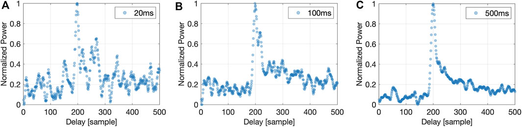
FIGURE 4. Waveform of the reflected signal with different incoherent integration of (A) 20 ms, (B) 100 ms, and (C) 500 ms.

As the number of incoherent integration increases, the waveform becomes clearer and the noise is smoothed at first. However, when the incoherence time reaches a certain threshold, the waveform gradually stabilizes and does not change any more. At this time, the SNR of the waveform also tends to be stable. The threshold is named as minimum saturation incoherent integration duration and is of great interest.

The minimum saturation incoherent integration duration varies for each observation due to variation of geometry and the reflected surface. An optimal integral duration should be determined that enables all observed waveforms to reach a steady state by making use of statistical methods. In the meanwhile, it should be verified that the sea level change within the duration is in an acceptable range. Based on the optimal integration duration, the clear waveform and thus accurate SSH estimation can be derived.

3.4 Estimation of path delay using delay waveform

3.4.1 Waveform retracking

The specular point in data is obtained by the Open Loop (OL) tracker. There is distortion between the OL derivation value and its ground-truth position due to real sea surface undulation relative to the mean sea surface (MSS) level. Hence, an accurate extraction of the specular point is necessary. The typical waveform tracking algorithm includes leading-edge-derivative (DER), the half-waveform method (HALF), and waveform fitting (FIT) (Rius et al., 2010; Cardellach et al., 2014; Li et al., 2018; Hu et al., 2020). Li has proven that DER and HALF methods show similar precision through model derivation and data verification, and the FIT method performs best but involves covariance calculation (Li et al., 2018, 2019). The HALF method is used here due to its efficiency. In addition, prior fraction $F_{sp}$ of the specular point is added as a correction item to retracking.

The prior information is obtained from the simulated waveform generated by the Z-V model implemented in WavPy open-source library (Fabra et al., 2017; Voronovich and Zavorotny, 2018). In waveform simulation, a series of parameters needs to be set:

1) The type of the GNSS signal is controlled by the weight of the GNSS composition.

2) The difference of GNSS-R instruments including front-end parameters is shown in Table 1 and antenna pattern (CYGNSS: a given 2-D map, TDS-1: spline interpolation).

3) The coherence time.

4) The sea surface wind speed is obtained from the European Centre for Medium-Range Weather Forecasts (ECMWF) ERA5 reanalysis data, and the mean sea surface slope is computed directly in the model.

Then, $F_{sp}$ is calculated in the modeled waveform:

${\mathit{F}}_{\mathit{s}\mathit{p}}=\frac{{\mathit{P}}_{\mathit{s}\mathit{p}}^{\mathit{mod}}-\mathit{N}}{{\mathit{P}}_{\mathit{max}}^{\mathit{mod}}-\mathit{N}},(6)$

in which, $P_{sp}^{\mathit{mod}}$ and $P_{\mathit{max}}^{\mathit{mod}}$ represent the power value at the specular point and the peak point, respectively, and $N$ is the noise floor. The nominal specular point could be obtained by the factor $F_{sp}$. Thus, the residual bistatic delay could be corrected by $∆t$:

$\left.{\mathit{P}}_{\mathit{s}\mathit{p}}^{\mathit{o}\mathit{b}\mathit{s}}={\mathit{F}}_{\mathit{s}\mathit{p}}\bullet {\left(\mathit{P}\right.}_{\mathit{max}}^{\mathit{o}\mathit{b}\mathit{s}}-\mathit{N}\right),(7)$

$∆\mathit{t}={\mathit{t}}_{\mathit{t}\mathit{r}\mathit{u}\mathit{e}}^{\mathit{o}\mathit{b}\mathit{s}}-{\mathit{t}}_{\mathit{s}\mathit{p}}^{\mathit{o}\mathit{b}\mathit{s}},(8)$

in which, $P_{sp}^{obs}$ and $P_{\mathit{max}}^{obs}$ represent the power value at the specular point and the peak point, respectively; $t_{true}^{obs}$ is the true delay of the specular point (red star in Figure 5) corresponding to power of $P_{sp}^{obs}$ in the leading-edge of observed waveform; and $t_{sp}^{obs}$ is the on-board calculated delay of the specular point (red dot in Figure 5) derived by the OL tracker.

FIGURE 5

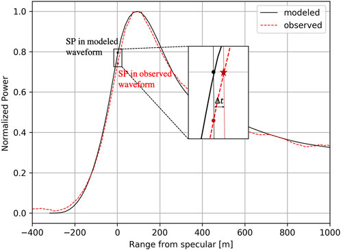
FIGURE 5. Example of an observed waveform with a comparison of a modeled waveform. The black dot is the specular point in a modeled waveform; the red dot is the OL specular point in the observed waveform; the red star is the true specular point in the observed waveform. The corrected item $∆t$ is the delay difference between the OL specular point and the true specular point in the observed waveform.

3.4.2 Atmospheric delay estimation

Due to the long-distance transmission and the discrepancy in the propagation path between the direct signal and the reflected signal, effects of the atmosphere on the received GNSS signals are inevitable. Errors caused by atmospheric effects include ionospheric and tropospheric delay errors. For obtaining an accurate altimetry result, these errors should be corrected.

Because current GNSS-R instruments used by the CYGNSS and TDS-1 are all of single frequency, the approach with the ionospheric-free combination eliminating ionospheric error is inapplicable; therefore, a reference ionospheric model is needed to remove the impact of the ionosphere. There are three ionospheric models commonly used: Klobuchar model (Klobuchar, 1987), international reference ionosphere (IRI) model (Bilitza, 2015), and IGS Global Ionospheric Total Electron Content Maps (GIMs) (Iijima et al., 1999). It has been found that the difference among these models is only 1–2 TECU, which is sub-meter corresponding to the range with the L1 C/A code, and the GIM is suggested for ionospheric correction of single-frequency altimeter observations for its stability (Jin, 2012). Here, the GIM model is used for estimating the ionospheric delay. The tropospheric delay is estimated at SP using the Saastamoinen model (Saastamoinen, 1972) and the Neil mapping function (Niell, 1996) with 2-meter temperature and mean sea-level pressure interpolated from ECMWF ERA5 reanalysis data and the water vapor calculated from the empirical, dimensional variable relative humidity in UNB3m (Leandro et al., 2006).

3.4.3 SSH observation retrieval

Once the delay path of SP is derived from the spaceborne-based raw IF data and the atmospheric delay is also estimated, SSH observation at the SP relative to the WGS-84 ellipsoid can be obtained by

$\mathit{S}\mathit{S}\mathit{H}=\frac{\left({\mathit{\rho }}_{\mathbf{2}}+{\mathit{\rho }}_{\mathit{m}}^{\mathit{i}\mathit{o}\mathit{n}}+{\mathit{\rho }}_{\mathit{m}}^{\mathit{t}\mathit{r}\mathit{o}}\right)-\left({\mathit{\rho }}_{\mathbf{1}}+{\mathit{\rho }}_{\mathit{s}\mathit{p}}\right)}{\mathbf{2}\mathit{sin}\mathit{\theta }}(9)$

where ${\rho }_{sp}$ is the ranging correction value of $∆t$ and ${\rho }_m^{ion}$ and ${\rho }_m^{tro}$ are the ionospheric and tropospheric delay, respectively.

It is important to note that, the coordinates of the receiver and the transmitter given in metadata are calculated based on the precise ephemeris results with a leap second; the undulation from Earth Gravitational Model 2008 (EGM 2008) should be considered for avoiding inaccurate values caused by the deviation between the real sea surface and the reference ellipsoid. In addition, the geometric information of the receiver and the transmitter should be synchronized to the same epoch because of the signal flight time (Hu et al., 2018). Then, the DTU18 mean sea surface (Andersen et al., 2018) is treated as the reference value to evaluate the GNSS-R based SSH results. The mean surface model represents the low-frequency component of ocean variation. To accurately evaluate GNSS-R based SSH precision, the tide error is also under consideration. The ocean and load tide are computed with the global ocean tide model (GOT4.10), and the solid tide is corrected by the IERS2003 model. The tide correction will be added to the reference sea level to evaluate the altimetry precision.

4 Results and discussion

4.1 Optimal integral duration

To evaluate the GNSS-R spaceborne ocean altimetry performance of multiple constellation signals and receiver platforms, the first step is the determination of optimal integral duration of the waveform. A summarization of the minimum saturation incoherent integral duration has been conducted using different transmitter signals separately.

By analyzing the datasets of the CYGNSS, for GPS L1 C/A signals, Galileo E1, and BDS B1 open service (OS) signals, incoherent integration time required for waveform stabilization and corresponding proportion is listed in Table 3; with incoherence time of 2,000 ms, 97% observations could achieve its maximum SNR and stable waveform for all three signals. To reduce altimetry retrieval error induced by insufficient incoherent integration, a resolution of 2s will be chosen and will satisfy the goal to study optimal ocean altimetry performance of multiple constellation signals.

TABLE 3

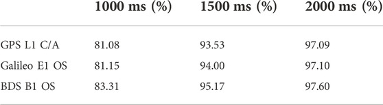
TABLE 3. Proportion of incoherence time to achieve stable signal quality.

Based on the DTU18 model, the mean sea surface height of 2s SP has been statistically analyzed, and 96% of the along-track MSS variation is within 0.8 m as shown in Figure 6. In such case, 2s or even higher resolution could be employed because the variation of reflection geometry and the reflecting surface properties induced by the spatial change is acceptable compared with the measuring accuracy of GNSS-R altimetry. Therefore, the final resolution of 2s (2,000 m incoherent integration) is used in the following analysis.

FIGURE 6

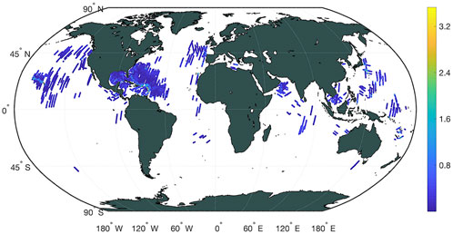
FIGURE 6. Along-track MSS variation of 2s specular points.

4.2 Altimetry performance of multiple constellation signals

Due to the differences in configuration of receiver radio frequency (RF) front-end and characteristics of GNSS signals, ocean altimetry performance is varying for different GNSS-R receivers. Previous analysis about the SNR with an integration duration of 1s shows that the mean SNRs from Galileo and BDS are 1∼2 dB lower than that from GPS; the mean SNRs of TDS-1 are 2∼4 dB lower than that of the CYGNSS, when the wind speed is as the same (Nan et al., 2021). In general, a higher SNR means better signal quality and higher altimetry precision. To assess the GNSS-R altimetry accuracy with an integration of 2s, the intertrack precision of 2s waveform is computed. It should be noted that the SSH measurements are converted to ranging to remove the dependency of elevation angle; and an adjustment method relying on prior MSS is implemented here as in Song et al. (2020), in which residual ranging errors are fitted with a cubic function to remove systematic errors and to analyze precision in one track. The ranging precision is expressed by the standard deviation (STD) after adjustment. Finally, the ranging precision and the mean SNR at SP of each track are fitted with an exponential function as a deformation of the analytical model of the statistics of the incoherently averaged waveform (Li et al., 2018):

$\mathit{S}\mathit{N}\mathit{R}=\mathbf{10}\bullet {\mathit{log}}_{\mathbf{10}}\frac{{\mathit{P}}_{\mathit{s}\mathit{p}}-\mathit{N}}{\mathit{N}},(10)$

${\mathit{\sigma }}_{\mathit{\rho }}^{\mathit{m}}=\mathit{a}\bullet {\mathit{e}}^{-\mathit{b}\bullet \mathit{S}\mathit{N}\mathit{R}}+\mathit{c},(11)$

where $P_{sp}$ is the power at the specular point and N is the noise floor of the waveform; ${\sigma }_{\rho }^m$ is the ranging precision; and a, b, and c are the coefficients of exponential fitting. The physical meaning of a corresponds to the ranging sensitivity which only depends on the autocorrelation properties of the transmitted signal (Li et al., 2018). After selection and procession, the data for ultimate analysis contain 181 tracks for CYGNSS—GPS $\left({CY}_G\right)$, 88 tracks for CYGNSS—Galileo $\left({CY}_E\right)$, 63 tracks from CYGNSS—BDS $\left({CY}_C\right)$, 282 tracks for TDS-1—GPS $\left({TDS}_G\right)$, and 53 tracks for TDS-1—Galileo $\left({TDS}_E\right)$.

The fitted curves for five groups are presented in Figure 7, and coefficients of the fitted curves are listed in Table 4. According to Figure 7, all the curves show the same pattern, i.e., the ranging precision improves with the increase of the waveform SNR; when the SNR is large enough, the variation reaches saturation and the curve converges, which means the random noise no longer dominates signal quality and the residual error comes from the altimetry algorithm and the instrument itself. In addition, the distribution of measurements of ${TDS}_G$ is more discrete than that of ${CY}_G$ as shown in Figure 7A and D, same for ${TDS}_E$ and ${CY}_E$ as shown in Figure 7B and E, which indicates TDS-1 data are more seriously contaminated by random noise and speckle noise. In addition, the mean SNR of CYGNSS data is -0.61 dB, which is consistent with the previous result derived by Li et al. (2019), while the mean SNR of TDS-1 is -1.82 dB. The higher SNR of the CYGNSS is closely linked to its better RF front-end and antenna configuration. In addition, since the orbit altitude of the CYGNSS satellite is lower than that of the TDS-1 satellite, the signal strength attenuation of the former, which is induced by propagation of the GNSS signal in the space, should be lower than that of the latter.

FIGURE 7

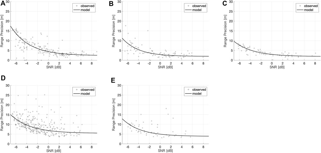
FIGURE 7. Observed ranging precision and the fitted model of 2s measurements for five groups: (A) for ${CY}_G$, (B) for ${CY}_E$, (C) for ${CY}_C$, (D) for ${TDS}_G$, and (E) for ${TDS}_E$.

TABLE 4

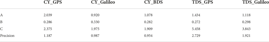
TABLE 4. Coefficients of the fitted curve and potential altimetry precision assuming the elevation angle of 30°.

From the fitted curve presented in Figure 7, the relationship of overall ranging precision among different satellite constellations is BDS > Galileo > GPS and CYGNSS > TDS-1, generally. From the aspect of fitted expression (11), a represents the amplitude of ranging precision, and its reciprocal is the ranging sensitivity in the meanwhile. Table 4 shows that Galileo/BDS is more sensitive in ranging than GPS due to a definitely smaller a value. The reason of this is that subcarriers are employed in Galileo/BDS E1/B1 OS original modulation, resulting in narrower (auto-correlation function) ACF main peak and steeper leading edge which accounts for the better sensitivity. The value c represents the final possible precision when the curve converges, and the SNR is large enough that the effect of random noise is fully eliminated. In CYGNSS datasets, the ultimate ranging precision can reach up to 2.375 m for GPS, 1.975 m for Galileo, and 1.909 m for BDS. Apparently, the performance of Galileo and BDS when the SNR in sufficient is better than that of GPS. In TDS-1 datasets, the ranging precision can reach up to 3.843 m for Galileo, which is better than that of GPS (5.458 m). Galileo and BDS show greater altimetry potential than GPS, although Galileo/BDS shows a lower SNR under the same wind speed due to smaller footprints as mentioned previously. It is explained that the pseudorandom ranging code length of the E1/B1 OS signal is several times greater than that of the GPS L1 C/A code (E1 by a factor of 4, B1 by a factor of 10), which could be understood as the E1/B1 OS signals have conducted observations repeatedly for one target, thus leading to better precision.

The improvement of potential ranging precision in ${TDS}_E$ compared to ${TDS}_G$ is 30%, while the one in ${CY}_E$ compared to ${CY}_G$ is about 17%. Galileo E1 signals show greater improvement in final possible precision in TDS-1 datasets. In these two groups of comparison separately, the receiver platform and RF front-end configuration are all fixed except for the receiver bandwidth of TDS-1 as presented in Table 1, which can be controlled by software to adjust the bandwidth to 4.2 MHz when receiving the Galileo signal. Therefore, this discrepancy should be caused by the adjustable receiver bandwidth with which the instrument onboard TDS-1 can capture the full bandwidth of the OS signals from Galileo, while the potential of Galileo/BDS OS signals is not fully developed in the CYGNSS for its narrower receiver bandwidth. That is, the receiver bandwidth is a great limitation for using the Galileo E1 signal for ocean altimetry in the CYGNSS, and it is supposed to achieve a better improvement in ranging precision in the future with a sufficient instrument bandwidth.

4.3 Coherent integration

Coherent integration is another effective method to increase signal processing gain and SNR. The navigation bit correction has already been conducted in raw IF data procession; thus, the I/Q component can be superimposed without considering phase reversal. The coherence time depends on coherence characteristics of the real reflected signal. A relationship between coherence and reflection geometry derived by Born and Wolf (2013)is asfollows:

${\mathit{T}}_{\mathit{c}}=\frac{\mathit{D}\mathit{i}\mathit{s}\mathit{t}\times \mathit{\lambda }}{\mathit{d}\mathit{i}\mathit{a}\mathit{m}\times \mathit{v}\mathit{e}\mathit{l}},(12)$

where Dist is the distance between the ‘active’ reflecting surface and the receiver; $\lambda$ is the carrier wavelength; diam is the equivalent diameter of the ‘active’ surface; and vel is the velocity of the receiver. For the first iso-delay ellipsoid, the E1/B1 OS signals apparently generate a smaller ‘active’ surface due to a wider bandwidth and narrower leading-edge, leading to a longer coherence time with respect to GPS L1. The influence of integer coherent integration (2 ms and 3 ms) on altimetry performance is assessed based on a 1-ms complex waveform. A same procedure as in Section 4.1 is conducted after coherent integration, and 2 ms coherent integration with 2,000 times incoherent accumulation, and 3 m coherent integration with 2,000 times incoherent accumulation are set. Longer coherent integration is unnecessary not only for limited bandwidth and coherence but also for more incoherent times required and low final resolution of SSH observations.

From Table 5, relevant conclusion can be drawn as follows:

TABLE 5

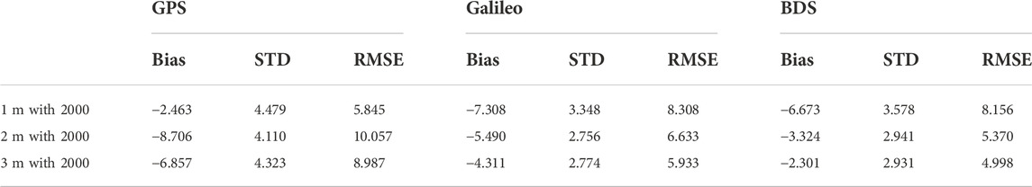
TABLE 5. Averaged SSH bias, STD, and root mean square error (RMSE) of each track for ${CY}_G$, ${CY}_E$, and ${CY}_C.$

For original 1 ms complex waveform directly conducting incoherent integration, extra negative bias is found both for ${CY}_E$ and ${CY}_C$, comparing to ${CY}_G$. In data procession, geometry model, and several corrections, no variable is concerned about the kind of transmitted signals. Only the integral processing method (longer coherence time) required by the E1/B1 OS signal and insufficient coherence time while processing complex waveform may contribute this SSH estimate anomaly.

After coherent integration, the bias is eliminated well for ${CY}_E$ and ${CY}_C$, which means more accurate single-point precision. This is because a shaper and clearer waveform could be obtained by coherent integration, facilitating the extraction of true SP accurately. The optimal coherence time depends on signal coherence. For CYGNSS-collected GPS L1 data, the result of 1 ms coherent integration shows a mean bias of -2.46 m, which is most likely due to the uncorrected ionospheric effect, orbit uncertainty, and other systematic errors. An extra bias is introduced with the increase of coherent integration as shown in the first three columns in Table 5. The coherence between L1 signal observations does not support longer coherence time, and the current 1 ms is a reasonable duration. Therefore, 1 ms results of GPS L1 signals are taken as the reference. For BDS B1 signals, the mean bias of 3 ms coherence time is -2.30 m, which is similar to the reference. The coherent integration has performed well for negative bias correction, and 3 ms is more suitable due to lower bias, STD, and RMSE. For the Galileo E1 signal, applying 2 ms and 3 ms coherence time, the bias is corrected to -5.49 m and -4.31 m. It is believed that there is still room for improvement, and higher coherence time could be considered but not tested in this analysis, limited by the length of a single data piece.

Comparing to only performing incoherent integration, the composition of coherent and incoherent integration absolutely performs better. In this case, incoherent integration is no longer the only factor affecting the signal quality and SSH measurement accuracy. In addition, the coherent integration is an effective way to increase SSH retrieval accuracy from the aspect of bias. On the other hand, this waveform processing strategy will sacrifice spatial resolution which should be balanced in realistic application.

5 Conclusion

GNSS-R is a promising technique because of the high spatial resolution of 5 km $\times$ 5 km and temporal resolution of mean revisit time of 7 hours and mid revisit time of 3 h, providing nearly gap-free Earth coverage. Although the altimetry accuracy technique is inferior than the traditional radar altimetry techniques, the GNSS-R-based SSH altimetry technique provides the possibility to measure mesoscale sea-surface height. With the increasing number of GNSS satellites, GNSS-R has gained increasing attention from the community.

This study presents the performance of the spaceborne GNSS-R code phase ocean altimetry with CYGNSS and TDS-1 collected GPS, Galileo, and BDS observations. By determining the optimal integration duration, their best altimetry precision is evaluated and compared using raw IF data. The raw IF data not only contain full waveform with higher delay resolution with respect to L1 data but also provide the opportunity to investigate the optimal integral duration for ocean altimetry with 1 ms observations. After extracting the waveform from raw IF datasets, a HALF method with model waveform simulated by WavPy library is applied to get the accurate position of SP in the waveform. Then, the geometry of spaceborne GNSS-R based SSH is implemented combined with several error corrections, such as ionospheric, tropospheric, and tide corrections to retrieve sea-surface height observations.

The determination of the optimal integral duration is fundamental for assessing the spaceborne GNSS-R ocean altimetry performance of multiple constellation signals. With current available data, through calculations about the along-track MSS variation and minimum integration time required to maximize the SNR of waveform, a resolution of 2s is adopted to satisfy most of the scenarios for GPS, BDS, and Galileo systems. After validation of the feasibility of GNSS-R ocean altimetry, the precision of five combinations of different receivers and transmitters is systematically analyzed by exponential fitting.

The results show that ocean altimetry accuracy is 2.375 m, 1.975 m, and 1.909 m for CYGNSS collected GPS L1, Galileo E1, and BDS B1 band signals, respectively, and the accuracy is 5.458 m and 3.843 m for TDS-1 collected GPS L1 and Galileo E1 band signals.

CYGNSS shows a more outstanding altimetry performance than TDS-1 in general due to the better configuration of RF front-end and the antenna pattern. In addition, the Galileo/BDS data are more sensitive to ranging than GPS due to their narrower leading-edge. Because of the shorter pseudorandom ranging code, the Galileo/BDS signals show better altimetry performance. A larger improvement between ${TDS}_G$ and ${TDS}_E$ in comparison with ${CY}_G$ and ${CY}_E$ indicates that receiver bandwidth is the main limitation for current GNSS-R ocean altimetry. In addition, the ionospheric delay error is still a limitation for ocean altimetry although partly calibrated by the GIM model, which is regarded as the main systematic error source.

Insufficient coherence integration leads to bias for signals from Galileo and BDS. In addition, the combined processing of coherent and incoherent integration is more efficient than pure incoherent integration. For Galileo and BDS E1/B1 OS signals, coherence time is higher than 3 ms, and 3 ms is suggested separately on the basis of 1 ms waveform, while current 1 ms coherence time is appropriate for GPS L1 signals.

As proved by Li et al. (2016), mesoscale sea surface features can be resolved down to 100 km using 2-day measurements of six receivers onboard COSMIC-2B. Similar spatial coverage and accuracy indicate the potential of the CYGNSS for resolving 2D mesoscale features to complement existing precision nadir altimeters. Meanwhile, based on the accuracy performance of the satellite system signals and the signal-to-noise ratio, the weight of a given satellite system can be determined, and by weighted averaging different satellite system-based SSH estimations, a higher precision SSH result can be obtained theoretically.

Data availability statement

Publicly available datasets were analyzed in this study. These data can be found here: https://www.ice.csic.es/gold_rtr_mining/gold_rtr.php.

Author contributions

TJ and XC initiated this study. ZC performed the data analysis, prepared all figures, and wrote the manuscript. XC and YL helped with the analysis. TJ and XW proposed suggestion on the result. All the authors reviewed the manuscript.

Funding

This study is supported by the National Natural Science Foundation of China under Grants 42192531, 42192534, and 41721003 and the Special Fund of Hubei Luojia Laboratory and the Foundation of Shanghai Academy of Spaceflight Technology under Grant SAST 2020–035.

Acknowledgments

The author would like to thank IEEC for providing processed IF datasets and Feixiong Huang for providing antenna pattern of CYGNSS mission.

Conflict of interest

The authors declare that the research was conducted in the absence of any commercial or financial relationships that could be construed as a potential conflict of interest.

Publisher’s note

All claims expressed in this article are solely those of the authors and do not necessarily represent those of their affiliated organizations, or those of the publisher, the editors, and the reviewers. Any product that may be evaluated in this article, or claim that may be made by its manufacturer, is not guaranteed or endorsed by the publisher.

References

Andersen, O., Knudsen, P., and Stenseng, L. (2018). “A new DTU18 MSS mean sea surface – improvement from SAR altimetry,” in 25 years of progress in radar altimetry symposium, Azores Archipelago, Portugal, September 2018, 172.

Google Scholar

Bilitza, D. (2015). The international reference Ionosphere – status 2013. Adv. Space Res. 55, 1914–1927. doi:10.1016/j.asr.2014.07.032

CrossRef Full Text | Google Scholar

Bindoff, N. L., Willebrand, J., Artale, V., Cazenave, A., Gregory, J. M., Gulev, S., et al. (2007). Observations: Oceanic climate change and sea level, 48. Lyon, France: Hal open science.

Google Scholar

Born, M., and Wolf, E. (2013). Principles of optics: Electromagnetic theory of propagation, interference and diffraction of light. Amsterdam, Netherlands: Elsevier.

Google Scholar

Cardellach, E., Rius, A., Martín-Neira, M., Fabra, F., Nogués-Correig, O., Ribó, S., et al. (2014). Consolidating the precision of interferometric GNSS-R ocean altimetry using airborne experimental data. IEEE Trans. Geosci. Remote Sens. 52, 4992–5004. doi:10.1109/TGRS.2013.2286257

CrossRef Full Text | Google Scholar

Clarizia, M. P., Pierdicca, N., Costantini, F., and Floury, N. (2019). Analysis of CYGNSS data for soil moisture retrieval. IEEE J. Sel. Top. Appl. Earth Obs. Remote Sens. 12, 2227–2235. doi:10.1109/JSTARS.2019.2895510

CrossRef Full Text | Google Scholar

Clarizia, M. P., Ruf, C., Cipollini, P., and Zuffada, C. (2016). First spaceborne observation of sea surface height using GPS-Reflectometry. Geophys. Res. Lett. 43, 767–774. doi:10.1002/2015GL066624

CrossRef Full Text | Google Scholar

Clarizia, M. P., and Ruf, C. S. (2016). Wind speed retrieval algorithm for the Cyclone global navigation satellite system (CYGNSS) mission. IEEE Trans. Geosci. Remote Sens. 54, 4419–4432. doi:10.1109/TGRS.2016.2541343

CrossRef Full Text | Google Scholar

Fabra, F., Cardellach, E., Li, W., and Rius, A. (2017). “Wavpy: A GNSS-R open source software library for data analysis and simulation,” in 2017 IEEE International Geoscience and Remote Sensing Symposium Fort Worth, TX, United States: IGARSS, 4125–4128. doi:10.1109/IGARSS.2017.8127908

CrossRef Full Text | Google Scholar

Fu, L.-L., Chelton, D. B., Le Traon, P.-Y., and Morrow, R. (2010). Eddy dynamics from satellite altimetry. Oceanogr. Wash. D. C 23, 14–25.Available at: https://www.jstor.org/stable/24860859 (Accessed September 12, 2022).

CrossRef Full Text | Google Scholar

Gleason, S., Hodgart, S., Sun, Y., Gommenginger, C., Mackin, S., Adjrad, M., et al. (2005). Detection and Processing of bistatically reflected GPS signals from low Earth orbit for the purpose of ocean remote sensing. IEEE Trans. Geosci. Remote Sens. 43, 1229–1241. doi:10.1109/TGRS.2005.845643

CrossRef Full Text | Google Scholar

Hajj, G. A., and Zuffada, C. (2003). Theoretical description of a bistatic system for ocean altimetry using the GPS signal. Radio Sci. 38–1019. doi:10.1029/2002RS002787

CrossRef Full Text | Google Scholar

Hu, C., Benson, C., Rizos, C., and Qiao, L. (2018). “An improved geometric model for space-based GNSS-R altimetry,” in IGARSS 2018 - 2018 IEEE International Geoscience and Remote Sensing Symposium, 3785–3788. doi:10.1109/IGARSS.2018.8518436

CrossRef Full Text | Google Scholar

Hu, C., Benson, C. R., Qiao, L., and Rizos, C. (2020). The validation of the weight function in the leading-edge-derivative path delay estimator for space-based GNSS-R altimetry. IEEE Trans. Geosci. Remote Sens. 58, 6243–6254. doi:10.1109/tgrs.2020.2975817

CrossRef Full Text | Google Scholar

Iijima, B. A., Harris, I. L., Ho, C. M., Lindqwister, U. J., Mannucci, A. J., Pi, X., et al. (1999). Automated daily process for global ionospheric total electron content maps and satellite ocean altimeter ionospheric calibration based on Global Positioning System data. J. Atmos. Solar-Terrestrial Phys. 61, 1205–1218. doi:10.1016/S1364-6826(99)00067-X

CrossRef Full Text | Google Scholar

Jales, P. (2015). Mission description - GNSS Reflectometry on TDS-1 with the SGR-ReSI, 26. Guildford, UK: Surrey Satellite Technology Limited.

Google Scholar

Jin, taoyong (2012). Cross-Calibration and errors analysis of Ionosphere correction in satellite altimetry. Geomatics Inf. Sci. Wuhan Univ. 37, 658–661.

Google Scholar

Klobuchar, J. A. (1987). Ionospheric time-delay algorithm for single-frequency GPS users. IEEE Trans. Aerosp. Electron. Syst. 23, 325–331. doi:10.1109/TAES.1987.310829

CrossRef Full Text | Google Scholar

Leandro, R., Santos, M., and Langley, R. (2006). UNB neutral atmosphere models: Development and performance. inAvailable at: http://www.ion.org/publications/abstract.cfm?jp=p&articleID=6562 (Accessed October 21, 2022).564573

Google Scholar

Levermann, A., Griesel, A., Hofmann, M., Montoya, M., and Rahmstorf, S. (2005). Dynamic sea level changes following changes in the thermohaline circulation. Clim. Dyn. 24, 347–354. doi:10.1007/s00382-004-0505-y

CrossRef Full Text | Google Scholar

Li, W., Cardellach, E., Ribó, S., Oliveras, S., and Rius, A. (2022). Exploration of multi-mission spaceborne GNSS-R raw IF data sets: Processing. Data Prod. Potential Appl. 24.

Google Scholar

Li, W., Fabra, F., Ribo, S., and Rius, A. (2020). Assessment of spaceborne GNSS-R ocean altimetry performance using CYGNSS mission raw data. IEEE Trans. Geosci. Remote Sens. 58, 238–250. doi:10.1109/tgrs.2019.2936108

CrossRef Full Text | Google Scholar

Li, W., Rius, A., Fabra, F., Cardellach, E., Ribó, S., and Martín-Neira, M. (2018). Revisiting the GNSS-R waveform statistics and its impact on altimetric retrievals. IEEE Trans. Geosci. Remote Sens. 56, 2854–2871. doi:10.1109/TGRS.2017.2785343

CrossRef Full Text | Google Scholar

Li, Z., Zuffada, C., Lowe, S. T., Lee, T., and Zlotnicki, V. (2016). Analysis of GNSS-R altimetry for mapping ocean mesoscale sea surface heights using high-resolution model simulations. IEEE J. Sel. Top. Appl. Earth Obs. Remote Sens. 9, 4631–4642. doi:10.1109/JSTARS.2016.2581699

CrossRef Full Text | Google Scholar

Lowe, S. T., Zuffada, C., Chao, Y., Kroger, P., Young, L. E., and LaBrecque, J. L. (2002). 5-cm-Precision aircraft ocean altimetry using GPS reflections. Geophys. Res. Lett. 29, 13-113–13-44. doi:10.1029/2002GL014759

CrossRef Full Text | Google Scholar

Lowe, S. T., Zuffada, C., LaBrecque, J. L., Lough, M., Lerma, J., and Young, L. E. (2000). “An ocean-altimetry measurement using reflected GPS signals observed from a low-altitude aircraft,” in IGARSS 2000. IEEE 2000 International Geoscience and Remote Sensing Symposium. Taking the Pulse of the Planet: The Role of Remote Sensing in Managing the Environment. Proceedings (Cat. No.00CH37120), Honolulu, HI, USA, July 2000, 2185–2187. vol. doi:10.1109/IGARSS.2000.8583505

CrossRef Full Text | Google Scholar

Martin-Neira, M. (1993). A passive reflectometry and interferometry system (PARIS): Application to ocean altimetry. ESA J. 17, 331–355.

Google Scholar

Martin-Neira, M., Caparrini, M., Font-Rossello, J., Lannelongue, S., and Vallmitjana, C. S. (2001). The PARIS concept: An experimental demonstration of sea surface altimetry using GPS reflected signals. IEEE Trans. Geosci. Remote Sens. 39, 142–150. doi:10.1109/36.898676

CrossRef Full Text | Google Scholar

Martin-Neira, M., Colmenarejo, P., Ruffini, G., and Serra, C. (2002). Altimetry precision of 1 cm over a pond using the wide-lane carrier phase of GPS reflected signals. Can. J. Remote Sens. 28, 394–403. doi:10.5589/m02-039

CrossRef Full Text | Google Scholar

Martin-Neira, M., Mavrocordatos, C., and Colzi, E. (1998). Study of a constellation of bistatic radar altimeters for mesoscale ocean applications. IEEE Trans. Geosci. Remote Sens. 36, 1898–1904. doi:10.1109/36.729361

CrossRef Full Text | Google Scholar

Nan, Y., Ye, S., Liu, J., Guo, B., Zhang, S., and Li, W. (2021). Signal-to-Noise ratio analyses of spaceborne GNSS-reflectometry from Galileo and BeiDou satellites. Remote Sens. 14, 35. doi:10.3390/rs14010035

CrossRef Full Text | Google Scholar

Niell, A. E. (1996). Global mapping functions for the atmosphere delay at radio wavelengths. J. Geophys. Res. 101, 3227–3246. doi:10.1029/95JB03048

CrossRef Full Text | Google Scholar

Picardi, G., Seu, R., Sorge, S. G., and Neira, M. M. (1998). Bistatic model of ocean scattering. IEEE Trans. Antennas Propag. 46, 1531–1541. doi:10.1109/8.725286

CrossRef Full Text | Google Scholar

Rius, A., Cardellach, E., and Martin-Neira, M. (2010). Altimetric analysis of the sea-surface GPS-reflected signals. IEEE Trans. Geosci. Remote Sens. 48, 2119–2127. doi:10.1109/tgrs.2009.2036721

CrossRef Full Text | Google Scholar

Ruf, C. S., Atlas, R., Chang, P. S., Clarizia, M. P., Garrison, J. L., Gleason, S., et al. (2016). New Ocean winds satellite mission to probe hurricanes and tropical convection. Bull. Am. Meteorol. Soc. 97, 385–395. doi:10.1175/BAMS-D-14-00218.1

CrossRef Full Text | Google Scholar

Ruf, C. S., Gleason, S., Jelenak, Z., Katzberg, S., Ridley, A., Rose, R., et al. (2012). “The CYGNSS nanosatellite constellation hurricane mission,” in 2012 IEEE International Geoscience and Remote Sensing Symposium, 214–216. doi:10.1109/IGARSS.2012.6351600

CrossRef Full Text | Google Scholar

Saastamoinen, J. (1972). Atmospheric correction for the troposphere and stratosphere in radio ranging satellites, The use of artificial satellites for geodesy. Washington, D.C, USA: American Geophysical Union AGU, 247–251. doi:10.1029/GM015p0247

CrossRef Full Text | Google Scholar

Song, M., He, X., Wang, X., Xiao, R., Shi, H., Wu, Y., et al. (2020). Study on the exploration of spaceborne GNSS-R raw data focusing on altimetry. IEEE J. Sel. Top. Appl. Earth Obs. Remote Sens. 13, 6142–6154. doi:10.1109/JSTARS.2020.3028693

CrossRef Full Text | Google Scholar

Treuhaft, R. N., Lowe, S. T., Zuffada, C., and Chao, Y. (2001). 2-cm GPS altimetry over crater lake. Geophys. Res. Lett. 28, 4343–4346. doi:10.1029/2001GL013815

CrossRef Full Text | Google Scholar

Unwin, M., Jales, P., Tye, J., Gommenginger, C., Foti, G., and Rosello, J. (2016). Spaceborne GNSS-reflectometry on TechDemoSat-1: Early mission operations and exploitation. IEEE J. Sel. Top. Appl. Earth Obs. Remote Sens. 9, 4525–4539. doi:10.1109/JSTARS.2016.2603846

CrossRef Full Text | Google Scholar

Voronovich, A. G., and Zavorotny, V. U. (2018). Bistatic radar equation for signals of opportunity revisited. IEEE Trans. Geosci. Remote Sens. 56, 1959–1968. doi:10.1109/TGRS.2017.2771253

CrossRef Full Text | Google Scholar

Yang, C., Miller, M., Nguyen, T., and Blasch, E. (2007). Comparative study of coherent, non-coherent, and semi-coherent integration schemes for GNSS receivers (preprint). Proc. Annu. Meet. - Inst. Navigation 20.

Google Scholar