Pseudo-depth domain reverse time migration in VTI medium based on GPU parallel strategy

As one of the main imaging methods, a lot of attention has been directed to reverse time migration anisotropic media. However, reverse time migration still faces cost and memory limitations, especially in imaging high frequencies. A coordinate transformation strategy in transversely isotropic media with a vertical axis of symmetry (VTI) was utilized to obtain high-resolution images useful for stratigraphic interpretation. The coordinate transformation converted traditional depth domain imaging into pseudo-depth domain imaging. In addition, this paper used the Graphics Processing Unit (GPU) parallel strategy and compared the imaging approach with the conventional acoustic isotropy method. By testing several models and field data, it concludes that Graphics Processing Unit parallel strategy can significantly improve the computational efficiency of imaging. The pseudo-depth domain method also has obvious advantages in computational time and memory consumption. Moreover, it is more reasonable when considering anisotropy for complex laminated layers.

1 Introduction

Reverse Time Migration (RTM) has been widely studied as an easy-to-implement, high-precision two-way wave equations migration imaging method. The finite difference method has better discrete characteristics, so it can be well expressed by computer language and be used for RTM. The RTM method is based on the principle of time consistency (Claerbout, 1971), which requires the calculation and storage of the wavefield at all times, and then cross-correlation imaging at each time point. Due to the inherent characteristics of this imaging strategy, this migration method brings an incredible burden on the capacity and calculation productivity of the computer. In particular, for deep layer data migration images, the RTM method requires huge calculations and memory allocation. At the same time, anisotropic complexity is caused by factors such as buried profundity within the vertical direction, which will influence the vertical complex structural imaging.

The RTM imaging method includes high-precision imaging characteristics, and its development has a long history. Whitmore (1983) used the results of RTM to pick up horizons and update the velocity model. The pseudo-spectral method is applied to realize RTM because of the computational efficiency and accuracy advantages (Baysal et al., 1983). To break through the inclination limit of the one-way wave equations, McMechan (1983) chose the finite difference method to solve the two-way wave equations. The excitation time imaging condition, or cross-correlation imaging condition, of RTM was developed, which was applied to vertical seismic profile (VSP) prestack data processing for the first time (Chang and McMechan, 1986). Sun and McMechan (1986) developed elastic wave prestack RTM and applied it to synthetic offset VSP imaging for multi-component data, and the strategy obtained good results. Chang and McMechan (1987); Chang and McMechan (1994) proposed the inverse time migration of elastic waves in two dimensions and three dimensions by finite difference method. Based on common shot gathers, Du et al. (2012) proposed a method to correct the polarity reversal phenomenon in elastic wave RTM. Combining migration with the idea of least squares, Dai et al. (2012) proposed the Least-Squares Reverse Time Migration (LSRTM). The LSRTM method for viscoelastic media (Yang and Zhu, 2019) and the LSRTM method for VTI media (Yang et al., 2019) are also proposed to compensate for the attenuation of viscoelastic media and obtain high-resolution imaging of anisotropic media. Mu et al. (2020a); Mu et al. (2020b) compared the fault tolerance of qP wave equations LSRTM results in tilted transverse isotropy (TTI) media with homogeneous isotropic media. The research also analyzed the sensitivity difference of this method to anisotropic parameters and tilted angles.

In view of the field data, the RTM method based on the finite difference method requires a huge amount of computation and needs a large memory, which is a big challenge when used in industry. Since the development of RTM, many scholars have done a lot of research on saving calculation costs and reducing memory consumption. Foltinek et al. (2009) combined the GPU parallel strategy with RTM, and a high-order finite-difference inverse time migration was realized. Suh et al. (2010) studied the strategy of parallel computing of inverse time migration based on clusters; Hayashi and Burns (1999) proposed the method of finite difference with a variable grid, which has unique advantages in realizing RTM and reducing storage demands. Symes (2007) proposed the checkpoint idea; this idea can save the source wavefield at a specific time and then extrapolate unknown source wavefields for imaging, thus reducing memory demands. Nguyen and McMechan (2013) proposed excitation amplitude imaging conditions. This method only needs to store the maximum amplitude and corresponds to travel time at each grid point, which greatly reduces the storage and input/output burden. Gu et al. (2015) developed a modified imaging condition of excitation amplitude prestack RTM, which saves memory consumption on the premise of ensuring accuracy. Wang et al. (2019); Wang et al. (2020) combined the variable grid method with the GPU parallel strategy and introduced it into FWI and LSRTM, which effectively improves the efficiency of the computation.

Since the pseudo-depth domain method was proposed, lots of corresponding research into migration and inversion has been discussed for oil and gas exploration. The main idea of the pseudo-depth domain method is to transform the computational domain and solve the new derived wave equation in a new computational domain (Alkhalifah et al., 2001). In vertical transversely isotropic media, the imaging is represented by vertical time instead of depth, thus eliminating the inherent ambiguity of analyzing vertical P-wave velocity from surface seismic data. Additionally, Alkhalifah (2003) discussed the advantages in velocity analysis of isotropic media. Ma and Alkhalifah (2013) derived the isotropic and anisotropic wave equations in the pseudo-depth domain and concluded that the pseudo-depth domain method can effectively improve computational efficiency and save memory. Plessix (2013) introduced the concept of the pseudo-depth domain into FWI, which can effectively avoid the ambiguity caused by velocity depth in VTI media. Li et al. (2017) and Sun et al. (2018) proposed a pseudo-depth domain cross-correlation least-squares inverse time migration method, which weakens the ambiguity of velocity and depth in traditional least-squares inverse time migration, improves the fault tolerance, computational efficiency, and reduces the memory occupied.

The literature review emphasizes the opportunity for future research. Anisotropy is a trend for future research on the imaging of complex subsurface structures. At the same time, the expensive computation and huge memory consumption of migration are problems that cannot be ignored. Under the condition of computational requirements, by redrawing the grid size in the vertical travel time domain to a certain extent, the pseudo-depth domain method eliminates the problem of speed wavelength mapping ambiguity caused by rigid spatial grid division and reduces the unnecessary grid memory occupation and computational load. A VTI medium mainly shows anisotropic response in vertical directions, which coincides with the idea of the pseudo-depth domain method in vertical transformation. This study developed the pseudo-depth domain RTM imaging method in a VTI medium and presents the GPU parallel computing methodology to further move forward computing efficiency and obtain a good application of the pseudo-depth domain method in VTI medium imaging. The effectiveness of the method was verified by several two-dimension numerical experiments and field data with different geological structures, which highlighted the advantages of the new strategy in computational time and memory cost.

The outline of this paper is structured as follows. Section 2 introduces the pseudo-depth domain mapping method and derives the first-order velocity stress wave equations of the VTI medium in the pseudo-depth domain. In addition, the pseudo-depth domain RTM (PDRTM) imaging workflow under the VTI medium is introduced, combined with the GPU parallel acceleration strategy. Section 3 introduces the pseudo shear wave suppression method in VTI media forward modeling under acoustic approximation. Furthermore, the accuracy and calculation cost of the depth domain method and the pseudo-depth domain method is compared. Section 4 points out that the pseudo-depth domain RTM of VTI media with GPU parallel has better imaging effect and computing efficiency, which can reduce memory consumption. The last section puts forward the conclusions and prospects.

2 Methods

The following section describes the implementation principles of VTI PDRTM method in detail, which are mainly divided into three parts: the derivation of wave equations in the VTI medium pseudo-depth domain, a review of the RTM imaging method, and CPU & GPU cooperative operation. Additionally, this method mainly depends on two key points: (1) the derivation of VTI wave equations using the pseudo-depth domain mapping method; (2) CPU and GPU cooperative calculation technology.

2.1 Pseudo-depth domain mapping principle and VTI medium wave equations derivation in pseudo-depth domain

The method of the pseudo-depth domain is to map the velocity field from the depth domain to the vertical time domain by coordinate transformation. We use the finite difference method to solve the transformed pseudo-depth domain wave equations. The mapping relationship between the depth domain and vertical time domain is introduced in more detail below. The main method of mapping is to transform the vertical depth domain coordinates $z$ into pseudo-depth domain coordinates $\tau$ (one-way wave vertical travel time):

$\tau \left(x,z\right)={\int }_0^z\frac{dz}{v_{sm}\left(x,z\right)}(1)$

Where $V_{sm}$ is the smooth velocity field at the corresponding vertical position. In the pseudo-depth domain, time grids are divided according to the smoothing speed of the corresponding position, which causes an uneven $d\tau$ distribution. In order to use the finite difference method to calculate, we needed to select the same size $\tau$ field sampling points artificially. In this paper, we used the spline interpolation method to obtain the pseudo-depth domain velocity field with the same vertical interval size. The interpolated velocity field was used for the following forward modeling and migration to avoid spatial aliasing; the interval $\Delta \tau$ should follow the sampling condition (Alkhalifah et al., 2001).

$\Delta \tau \le \frac{v_{\min }}{10f_{\max }}(2)$

Where $v_{\min }$ is the minimum velocity in the calculation area and $f_{\max }$ is the maximum frequency of the seismic wave. Due to coordinate transformation, the number of longitudinal sampling points is no longer equal to the number of sampling points $n_z$ in the depth domain, and the number of sampling points $n_{\tau }$ in the pseudo-depth domain follow the condition:

$n_{\tau }\Delta \tau \ge {\tau }_{\max }\left(x,z\right)(3)$

Where ${\tau }_{\max }\left(x,z\right)$ is the maximum value of 1-D one-way travel time of each trace obtained by Equation 1. Only when the sampling points satisfy the conditions in Equation 3 can the data ensure integrity in the process of coordinate mapping, otherwise it will lead to missing data. Of course, after the inversion or imaging of the data, it is necessary to transform the processed data back to the depth domain.

$z\left(x,\tau \right)={\int }_0^{\tau }{v}_{sm}\left(x,\tau \right)d\tau (4)$

In fact, transforming depth domain $z$ into the pseudo-depth domain is to convert $\left(x,z\right)$ into $\left(\xi ,\eta \right)$ through coordinate mapping, as shown in Figure 1. This makes it possible to use finer spatial sampling in the low-speed zone and larger spatial sampling in the high-speed zone, thereby avoiding the waste of computing resources. When each time point is calculated, the wavefield occupies the compressed grid’s number.

FIGURE 1

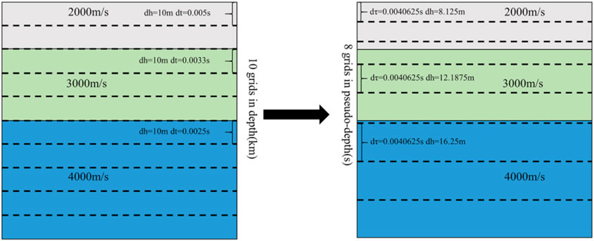
FIGURE 1. Schematic diagram of pseudo-depth domain transformation principle in depth domain.

Next, we derived the wave equations of the VTI medium in the pseudo-depth domain. The transformation is carried out in the vertical direction as follows:

$\left\{\begin{array}{c}\xi =x\\ \eta =\tau \end{array}\right.(5)$

Assuming that the stress field in the Cartesian coordinate system is $P_z\left(x,z\right)$, then the stress field in pseudo-depth domain becomes $P_{\tau }\left(\xi ,\eta \right)$. The derivative transformation is written as follows:

$\left\{\begin{array}{c}{F}_x=\frac{\partial F}{\partial x}\\ F_{xy}=F_{yx}=\frac{{\partial }^{2}F}{\partial x\partial y}\end{array}\right.(6)$

By combining Equation 6 with (5), there are:

$\left\{\begin{array}{c}{\xi }_x=\frac{\partial \xi }{\partial x}=\frac{\partial x}{\partial x}=1\\ {\xi }_z=\frac{\partial \xi }{\partial z}=\frac{\partial x}{\partial z}=0\\ {\eta }_x=\frac{\partial \eta }{\partial x}=\frac{\partial \tau }{\partial x}\\ {\eta }_z=\frac{\partial \eta }{\partial z}=\frac{\partial \tau }{\partial z}=\frac{1}{v_{sm}}\end{array}\right.(7)$

Let ${\eta }_x=\alpha$, Equation 7 is equivalent to the Jacobian determinant:

$\mathrm{J}=\left[\begin{array}{c}\begin{array}{cc}{\xi }_x& {\xi }_z\end{array}\\ \begin{array}{cc}{\eta }_x& {\eta }_z\end{array}\end{array}\right]=\left[\begin{array}{cc}\begin{array}{c}1\\ \frac{\partial \tau }{\partial x}\end{array}& \begin{array}{c}0\\ \frac{1}{v_{sm}}\end{array}\end{array}\right]=\left[\begin{array}{cc}\begin{array}{c}1\\ \alpha \end{array}& \begin{array}{c}0\\ \frac{1}{v_{sm}}\end{array}\end{array}\right](8)$

From the Jacobian determinant, the diagonal elements are non-zero, which means that the coordinate $\tau$ is non-orthogonal. Therefore, the matrix tensor can be calculated:

$g^{ij}=J{J}^T=\left[\begin{array}{cc}1& \frac{\partial \tau }{\partial x}\\ \frac{\partial \tau }{\partial x}& \frac{1}{{V_{sm}}^2}+{\left(\frac{\partial \tau }{\partial x}\right)}^2\end{array}\right]=\left[\begin{array}{cc}1& \alpha \\ \alpha & \frac{1}{{V_{sm}}^2}+{\alpha }^2\end{array}\right](9)$

$\left|g_{ij}\right|={\left(g^{ij}\right)}^{-1}=\frac{1}{\det \left(g^{ij}\right)}={V_{sm}}^2(10)$

From the above equations, let $\sqrt{g}=v_{sm}$. The two-way wave equations can be written in the following first-order form.

$\left\{\begin{array}{c}\frac{\partial p}{\partial t}=v^2\nabla ·\mathit{q}\\ \frac{\partial \mathit{q}}{\partial t}=\nabla p\end{array}\right.(11)$

Where, $P$ is the stress field and $\mathit{q}$ is the strain field.

Suppose that the unit basis vector in the coordinate $\left(\xi ,\eta \right)$ system is $\left(e_1,e_2\right)$. When the basis vector and the matrix tensor are known, the gradient in the new coordinate system can be expressed as (Riley and Hobson, 2006; Ma and Alkhalifah, 2013):

$\nabla p=p_{\xi }{g}^{11}{e}_1+p_{\xi }{g}^{21}{e}_2+p_{\eta }{g}^{12}{e}_1+p_{\eta }{g}^{22}{e}_2(12)$

Combining Equation 9 with Equation 12, the above equation can be simplified as:

$\nabla p=\left(p_{\xi }+\alpha p_{\eta }\right)e_1+\left(\alpha p_{\xi }+{\alpha }^2{p}_{\eta }+\frac{1}{v_{sm}2}{p}_{\eta }\right)e_2(13)$

For vectors $\mathit{q}={\mathit{q}}_x{e}_1+{\mathit{q}}_z{e}_2$, divergence can be expressed as:

$\nabla ·\mathit{q}=\frac{1}{\sqrt{g}}\frac{\partial }{\partial \xi }\left(\sqrt{g}{\mathit{q}}_x\right)+\frac{1}{\sqrt{g}}\frac{\partial }{\partial \eta }\left(\sqrt{g}{\mathit{q}}_z\right)(14)$

Combining Equation 10 with Equation 14, the above equation can be expressed as:

$\nabla ·\mathit{q}=\frac{1}{v_{sm}}\frac{\partial }{\partial \xi }\left(v_{sm}{\mathit{q}}_x\right)+\frac{1}{v_{sm}}\frac{\partial }{\partial \eta }\left(v_{sm}{\mathit{q}}_z\right)(15)$

Therefore, for the acoustic isotropy medium, the first-order velocity stress equations (Virieux, 1984; Virieux, 1986) are shown as follows:

$\left\{\begin{array}{c}\frac{1}{\rho v^2}\frac{\partial P}{\partial t}=\frac{\partial u}{\partial x}+\frac{\partial w}{\partial z}\\ \frac{1}{\rho }\frac{\partial P}{\partial z}=\frac{\partial w}{\partial t}\\ \frac{1}{\rho }\frac{\partial P}{\partial x}=\frac{\partial u}{\partial t}\end{array}\right.(16)$

P is the acoustic pressure stress field, and u and w represent the strain in the x and z directions, respectively. The form of the pseudo-depth domain derived from Equations 13, 15, 16 can be written as follows:

$\left\{\begin{array}{c}\rho \frac{\partial u}{\partial t}=\frac{\partial p}{\partial \xi }+\alpha \frac{\partial p}{\partial \eta }\\ \rho \frac{\partial w}{\partial t}=\alpha \frac{\partial p}{\partial \xi }+\left({\alpha }^2+\frac{1}{{V_{sm}}^2}\right)\frac{\partial p}{\partial \eta }\\ \frac{\partial p}{\partial t}=\frac{\rho v^2}{v_{sm}}\left[\frac{\partial \left(v_{sm}u\right)}{\partial \xi }+\frac{\partial \left(v_{sm}w\right)}{\partial \eta }\right]\end{array}\right.(17)$

By Taylor expansion, the discrete form is obtained:

$\left\{\begin{array}{c}{P}_{i,j}^{k+\frac{1}{2}}=P_{i,j}^{k-\frac{1}{2}}+\frac{\Delta t\rho v^2}{v_{\mathrm{s}\mathrm{m}}\Delta x}\left\{{\displaystyle \sum }_{m=1}^L{a}_m\left[V_{i+\frac{2m-1}{2},j}^k{U}_{i+\frac{2m-1}{2},j}^k-V_{i-\frac{2m-1}{2},j}^k{U}_{i-\frac{2m-1}{2},j}^k\right]\right\}\\ +\frac{\Delta t\rho v^2}{v_{\mathrm{s}\mathrm{m}}\Delta \tau }\left\{{\displaystyle \sum }_{m=1}^L{a}_m\left[V_{i,j+\frac{2m-1}{2}}^k{W}_{i,j+\frac{2m-1}{2}}^k-V_{i,j-\frac{2m-1}{2}}^k{W}_{i,j-\frac{2m-1}{2}}^k\right]\right\}\\ U_{i+\frac{1}{2}.j}^k=U_{i+\frac{1}{2},j}^{k-1}+\frac{\Delta t}{\rho \Delta x}\left\{{\displaystyle \sum }_{m=1}^L{a}_m\left[P_{i+\frac{1}{2}+\frac{2m-1}{2},j}^{k-\frac{1}{2}}-P_{i+\frac{1}{2}-\frac{2m-1}{2},j}^{k-\frac{1}{2}}\right]\right\}\\ +\frac{\alpha \Delta t}{\rho \Delta \tau }\left\{{\displaystyle \sum }_{m=1}^L{a}_m\left[P_{i,j+\frac{1}{2}+\frac{2m-1}{2}}^{k-\frac{1}{2}}-P_{i,j+\frac{1}{2}-\frac{2m-1}{2}}^{k-\frac{1}{2}}\right]\right\}\\ W_{i,j+\frac{1}{2}}^k=W_{i,j+\frac{1}{2}}^{k-1}+\frac{\alpha \Delta t}{\rho \Delta x}\left\{{\displaystyle \sum }_{m=1}^L{a}_m\left[P_{i+\frac{1}{2}+\frac{2m-1}{2},j}^{k-\frac{1}{2}}-P_{i+\frac{1}{2}-\frac{2m-1}{2},j}^{k-\frac{1}{2}}\right]\right\}\\ +\left({\alpha }^2+\frac{1}{v_{\mathrm{s}\mathrm{m}}^2}\right)\frac{\Delta t}{\rho \Delta \tau }\left\{{\displaystyle \sum }_{m=1}^L{a}_m\left[P_{i,j+\frac{1}{2}+\frac{2m-1}{2}}^{k-\frac{1}{2}}-P_{i,j+\frac{1}{2}-\frac{2m-1}{2}}^{k-\frac{1}{2}}\right]\right\}\end{array}\right.(18)$

Where P is acoustic pressure field, U and W are strain variables, $\rho$ represents density, m is the finite difference order, i and j are the positions of grid points in the transverse and longitudinal directions, and $a_m$ is the finite difference coefficients.

This paper studies the wavefield characteristics and migration methods in VTI media, using the first-order velocity stress equations of VTI (Duveneck et al., 2008) under acoustic approximation:

$\left\{\begin{array}{c}\frac{1}{\rho {V_P}^2}\frac{\partial P_H}{\partial t}=\left(1+2\epsilon \right)\frac{\partial u}{\partial x}+\sqrt{1+2\delta }\frac{\partial w}{\partial z}\\ \frac{1}{\rho {V_P}^2}\frac{\partial P_V}{\partial t}=\sqrt{1+2\delta }\frac{\partial u}{\partial x}+\frac{\partial w}{\partial z}\\ \frac{\partial u}{\partial t}=\frac{1}{\rho }\frac{\partial P_H}{\partial x}\\ \frac{\partial w}{\partial t}=\frac{1}{\rho }\frac{\partial P_V}{\partial z}\end{array}\right.(19)$

Where $P_H$ and $P_V$ represent the horizon and vertical stress fields, $\delta$ and $\epsilon$ represent the anisotropic parameters. Similar to the above method of deriving pseudo-depth domain, the first-order velocity stress equations of VTI can be deduced to pseudo-depth domain by Equations 13, 15, 19:

$\left\{\begin{array}{c}\frac{1}{\rho {V_P}^2}\frac{\partial P_H}{\partial t}=\left(1+2\epsilon \right)\left(\frac{\partial u}{\partial \xi }+\alpha \frac{\partial u}{\partial \eta }\right)+\sqrt{1+2\delta }\frac{1}{v_{sm}}\frac{\partial w}{\partial \eta }\\ \frac{1}{\rho {V_P}^2}\frac{\partial P_V}{\partial t}=\sqrt{1+2\delta }\left(\frac{\partial u}{\partial \xi }+\alpha \frac{\partial u}{\partial \eta }\right)+\frac{1}{v_{sm}}\frac{\partial w}{\partial \eta }\\ \frac{\partial u}{\partial t}=\frac{1}{\rho }\left(\frac{\partial P_H}{\partial \xi }+\alpha \frac{\partial P_H}{\partial \eta }\right)\\ \frac{\partial w}{\partial t}=\frac{1}{\rho }\frac{1}{v_{sm}}\frac{\partial P_V}{\partial \eta }\end{array}\right.(20)$

In practice, the parameters of vertical anisotropy are quite complex, so it is necessary to combine well-logging information with petrophysical experiments to obtain different empirical equations. In the following content of model test, Gardner’s empirical equation is used to calculate the anisotropic parameter field.

$\left\{\begin{array}{c}\rho =0.31\cdot {V_p}^{0.25}\cdot 1000\\ \epsilon =0.25\frac{\rho }{1000}-0.3\\ \delta =0.125\frac{\rho }{1000}-0.1\end{array}\right.(21)$

Similarly, for the convenience of computer expression, Taylor expansion is used to derive the discrete form:

$\left\{\begin{array}{c}{P}_{i,j}^{k+\frac{1}{2}}=P_{i,j}^{k-\frac{1}{2}}+{\rho v_p}^2\left(1+2\epsilon \right)\{\frac{\Delta t}{\Delta x}{\displaystyle \sum }_{m=1}^L{a}_m\left[U_{i+\frac{2m-1}{2},j}^k-U_{i-\frac{2m-1}{2},j}^k\right]\\ +\alpha \frac{\Delta t}{\Delta \tau }{\displaystyle \sum }_{m=1}^L{a}_m\left[U_{i+\frac{2m-1}{2},j}^k-U_{i-\frac{2m-1}{2},j}^k\right]\}\\ +\frac{\Delta t\rho {v_p}^2\sqrt{1+2\delta }}{v_{\mathrm{s}\mathrm{m}}\Delta \tau }\left\{{\displaystyle \sum }_{m=1}^L{a}_m\left[W_{i,j+\frac{2m-1}{2}}^k-W_{i,j-\frac{2m-1}{2}}^k\right]\right\}\\ Q_{i,j}^{k+\frac{1}{2}}=Q_{i,j}^{k-\frac{1}{2}}+{\rho v_p}^2\sqrt{\left(1+2\delta \right)}\{\frac{\Delta t}{\Delta x}{\displaystyle \sum }_{m=1}^L{a}_m\left[U_{i+\frac{2m-1}{2},j}^k-U_{i-\frac{2m-1}{2},j}^k\right]\\ +\alpha \frac{\Delta t}{\Delta \tau }{\displaystyle \sum }_{m=1}^L{a}_m\left[U_{i+\frac{2m-1}{2},j}^k-U_{i-\frac{2m-1}{2},j}^k\right]\}\\ +\frac{\Delta t\rho {v_p}^2}{v_{\mathrm{s}\mathrm{m}}\Delta \tau }\left\{{\displaystyle \sum }_{m=1}^L{a}_m\left[W_{i,j+\frac{2m-1}{2}}^k-W_{i,j-\frac{2m-1}{2}}^k\right]\right\}\\ U_{i+\frac{1}{2}.j}^k=U_{i+\frac{1}{2},j}^{k-1}+\frac{\Delta t}{\rho \Delta x}\left\{{\displaystyle \sum }_{m=1}^L{a}_m\left[P_{i+\frac{1}{2}+\frac{2m-1}{2},j}^{k-\frac{1}{2}}-P_{i+\frac{1}{2}-\frac{2m-1}{2},j}^{k-\frac{1}{2}}\right]\right\}\\ +\frac{\alpha \Delta t}{\rho \Delta \tau }\left\{{\displaystyle \sum }_{m=1}^L{a}_m\left[P_{i,j+\frac{1}{2}+\frac{2m-1}{2}}^{k-\frac{1}{2}}-P_{i,j+\frac{1}{2}-\frac{2m-1}{2}}^{k-\frac{1}{2}}\right]\right\}\\ W_{i,j+\frac{1}{2}}^k=W_{i,j+\frac{1}{2}}^{k-1}+\frac{\alpha \Delta t}{\rho v_{sm}\Delta \tau }\left\{{\displaystyle \sum }_{m=1}^L{a}_m\left[Q_{i+\frac{1}{2}+\frac{2m-1}{2},j}^{k-\frac{1}{2}}-Q_{i+\frac{1}{2}-\frac{2m-1}{2},j}^{k-\frac{1}{2}}\right]\right\}\end{array}\right.(22)$

2.2 The review of RTM theory

Claerbout (1971) proposed that the core of RTM is time consistency. The imaging conditions based on this principle of migration are given as follows:

$R\left(x,y,z;s\right)=\frac{U\left(x,y,z;t;s\right)}{D\left(x,y,z;t;s\right)}(23)$

Where, R, U, and D represent the imaging result, the wavefield of receiver, and the wavefield of source, respectively. $\left(x,y,z\right)$ are the grid point position in the calculation area, $s$ is the source, and $t$ is the first arrival time. Since the denominator of Equation 23 is zero at the non-interface position, Claerbout (1971) used the zero delay cross-correlation of up and down traveling waves to obtain a stable imaging profile:

$R\left(x,y,z;s_j\right)={\displaystyle \sum }_j^{s_{\max }}{\displaystyle \sum }_i^{t_{\max }}U\left(x,y,z;t_i;s_j\right)D\left(x,y,z;t_i;s_j\right)(24)$

The RTM method is imaged by the principle of time consistency, which uses the extended source wavefield and receiver wavefield (as shown by Figure 2). The basic steps are as follows: (1) the source wavefield propagates forward; (2) the wavefield of the receiver point propagates backward; (3) zero delay cross-correlation between forward and backward wavefields are performed to obtain imaging results.

FIGURE 2

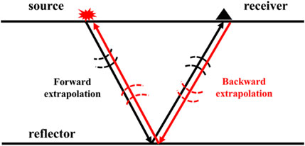
FIGURE 2. Diagram of seismic wavefield extrapolation.

The imaging condition used in this paper is the source normalized cross-correlation imaging condition proposed by Kaelin and Guitton (2006). Using the illumination of the source wavefield to normalize the cross-correlation imaging section can effectively reduce the influence of the source on the migration results.

$R\left(x,y,z;s_j\right)=\frac{\sum \sum U\left(x,y,z;t_i;s_j\right)D\left(x,y,z;t_i;s_j\right)}{\sum \sum D^2\left(x,y,z;t_i;s_j\right)}(25)$

The GPU VTI PDRTM method workflow is given in Figure 3. The specific process of VTI PDRTM model test is given here. First, the research obtained true seismic data through the VTI forward modeling of the real velocity field, using the data as the input of the inverse time extension of the wavefield at the receiver point. Second, the research used the smoothed velocity field to simulate the migration velocity field obtained by migration velocity analysis or tomography inversion. Meanwhile, the corresponding anisotropic parameters in model testing were obtained by Gardner’s empirical equation. The coordinate mapping of the obtained parameter field was used as the input of the forwarding extension of the seismic source wavefield. Third, the wave equations in the pseudo-depth domain in the VTI medium were used to carry out an inverse time extension and forward extension of the receiver wavefield and source wavefield. The extended wavefield was imaged under cross-correlation imaging conditions. Last, the final depth domain imaging profile was obtained by back-projection of the pseudo-depth domain imaging results.

FIGURE 3

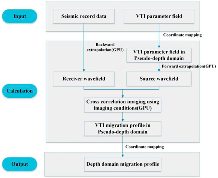
FIGURE 3. VTI pseudo-depth domain reverse time migration based on GPU parallel accelerated workflow.

2.3 CPU & GPU cooperative computing method

GPUs have powerful parallel computing capability. CUDA-C programming technology realizes the interaction between a GPU and its central processing unit (CPU), with the serial logic judgment, data reading, and writing part being put on the CPU. Finite difference parallel computing is handed over to the GPU, which can greatly improve computing efficiency. CUDA is composed of three software levels of grid-block-thread architecture, which corresponds to the three GPU hardware levels of the device-streaming multiprocessor (SM)-core. The CUDA software levels architecture is shown in Figure 4. In this paper, we put the finite difference operation part on the GPU and transferred data between the CPU and GPU through CUDA command.

FIGURE 4

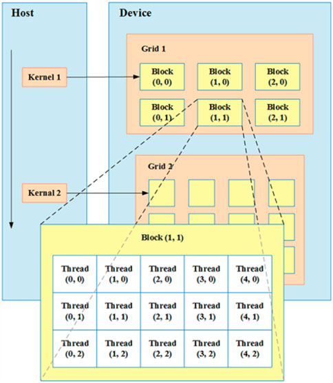
FIGURE 4. CUDA architecture.

In the two-dimension case, the position of each thread is determined by the index. The index in x and z directions can be expressed as:

$\mathrm{t}\mathrm{i}\mathrm{d}=\left(\mathrm{b}\mathrm{l}\mathrm{o}\mathrm{c}\mathrm{k}\mathrm{I}\mathrm{d}\mathrm{x}.\mathrm{x}*\mathrm{b}\mathrm{l}\mathrm{o}\mathrm{c}\mathrm{k}\mathrm{D}\mathrm{i}\mathrm{m}.\mathrm{x}\right)+\mathrm{t}\mathrm{h}\mathrm{r}\mathrm{e}\mathrm{a}\mathrm{d}\mathrm{I}\mathrm{d}\mathrm{x}.\mathrm{x}$

$\mathrm{t}\mathrm{i}\mathrm{d}=\left(\mathrm{b}\mathrm{l}\mathrm{o}\mathrm{c}\mathrm{k}\mathrm{I}\mathrm{d}\mathrm{x}.\mathrm{y}*\mathrm{b}\mathrm{l}\mathrm{o}\mathrm{c}\mathrm{k}\mathrm{D}\mathrm{i}\mathrm{m}.\mathrm{y}\right)+\mathrm{t}\mathrm{h}\mathrm{r}\mathrm{e}\mathrm{a}\mathrm{d}\mathrm{I}\mathrm{d}\mathrm{x}.\mathrm{y}$

The CUDA data transmission command is as follows:

$\mathrm{c}\mathrm{u}\mathrm{d}\mathrm{a}\mathrm{M}\mathrm{e}\mathrm{m}\mathrm{c}\mathrm{p}\mathrm{y}\left(\mathrm{a},\mathrm{b},\mathrm{n}\mathrm{u}\mathrm{m}1*\mathrm{n}\mathrm{u}\mathrm{m}2*\mathrm{s}\mathrm{i}\mathrm{z}\mathrm{e}\mathrm{o}\mathrm{f}\left(\mathrm{f}\mathrm{l}\mathrm{o}\mathrm{a}\mathrm{t}\right),\mathrm{c}\mathrm{u}\mathrm{d}\mathrm{a}\mathrm{M}\mathrm{e}\mathrm{m}\mathrm{c}\mathrm{p}\mathrm{y}\mathrm{H}\mathrm{o}\mathrm{s}\mathrm{t}\mathrm{T}\mathrm{o}\mathrm{D}\mathrm{e}\mathrm{v}\mathrm{i}\mathrm{c}\mathrm{e}\right)$

$\mathrm{c}\mathrm{u}\mathrm{d}\mathrm{a}\mathrm{M}\mathrm{e}\mathrm{m}\mathrm{c}\mathrm{p}\mathrm{y}\left(\mathrm{b},\mathrm{a},\mathrm{n}\mathrm{u}\mathrm{m}1*\mathrm{n}\mathrm{u}\mathrm{m}2*\mathrm{s}\mathrm{i}\mathrm{z}\mathrm{e}\mathrm{o}\mathrm{f}\left(\mathrm{f}\mathrm{l}\mathrm{o}\mathrm{a}\mathrm{t}\right),\mathrm{c}\mathrm{u}\mathrm{d}\mathrm{a}\mathrm{M}\mathrm{e}\mathrm{m}\mathrm{c}\mathrm{p}\mathrm{y}\mathrm{D}\mathrm{e}\mathrm{v}\mathrm{i}\mathrm{c}\mathrm{e}\mathrm{T}\mathrm{o}\mathrm{H}\mathrm{o}\mathrm{s}\mathrm{t}\right)$

3 Results

3.1 VTI acoustic approximate equations forward modeling and pseudo shear wave suppression

This part was based on VTI acoustic wave approximation equations to simulate in a homogeneous medium. Forward modeling was the basis of migration imaging. Therefore, only by accurately simulating the wavefield propagation process could the accuracy of imaging results be ensured. Wavefield characteristics of VTI were simulated, and the results are shown in Figure 5. It can be clearly seen that strong pseudo shear wave interference was generated in the acoustic approximate equations of VTI medium forward modeling. This interference needed to be effectively suppressed before the migration. We suppressed pseudo shear wave interference by loading the source loop near the source, assuming that the source was isotropic $\left(\epsilon =\delta =0\right)$ or elliptical anisotropic $\left(\epsilon =\delta \right)$ (Duveneck et al., 2008). This method was used to eliminate the pseudo shear wave interference in VTI imaging in the following content. The wavefield snapshot in Figure 5 adopted a model size of 6000m × 6000m, with the source set in the precise middle. The velocity and anisotropy parameters of the model were $v=4000\mathrm{m}\mathrm{s}$, $\epsilon =0.316,\delta =0.208$, respectively, and the output time was t=0.6s. It is obvious that Figure 5B has clear pseudo shear wave interference in the middle. In Figure 5C, the pseudo shear wave interference has been well suppressed. The shot record in Figure 6 adopted the method that sets shot at the surface midpoint, from which it can also be seen that the pseudo shear wave interference was suppressed.

FIGURE 5

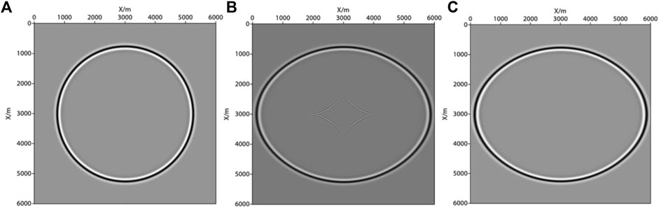
FIGURE 5. Snapshot of wavefield in forward modeling at 0.6s. (A) acoustic isotropy wave equations; (B) VTI acoustic wave approximate equations (without source loop); (C) VTI acoustic wave approximate equations (adding source loop).

FIGURE 6

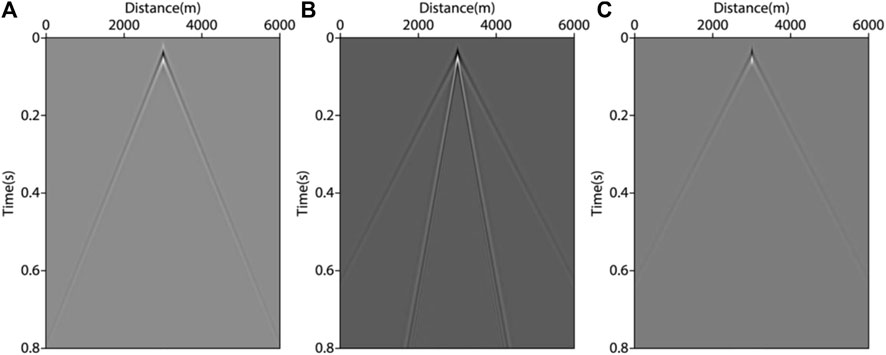
FIGURE 6. Shot records of forward modeling. (A) acoustic isotropy wave equations; (B) VTI acoustic wave approximate equations (without source loop); (C) VTI acoustic wave approximate equations (adding source loop).

3.2 Accuracy analysis of forward modeling in depth domain and pseudo-depth domain

In this part, the forward modeling records in depth domain and pseudo-depth domain were compared and analyzed. The significance of comparison in the two coordinates highlighted that the shot records systems did not change after coordinating mapping, which was an important basis for judging whether the migration method could be carried out later. Firstly, based on the real underground structure of a certain Sheng Li (SL) area, the SL velocity model (as shown in Figure 7A) was constructed, and the pseudo-depth domain transformation method was used to transform the model into the pseudo-depth domain (as shown in Figure 7B). The purpose of converting the velocity field to the pseudo-depth domain was to compare the forward modeling accuracy with the depth domain method. Secondly, in the CPU, the depth domain forward modeling and pseudo-depth domain forward modeling were carried out by using the finite difference method. The size of the velocity field was 4810m × 3060 m, with a vertical and horizontal grid spacing of 10 m. In order to facilitate comparison, the same observation system was used. Setting sources and receivers on the surface, the shot point was set at the midpoint of the ground, and there are 481 receivers on the surface with spacing of 10 m. The main frequency of the source was 20Hz, with a vertical and horizontal grid spacing of 10 m. The time sampling interval was 0.6 ms, with a maximum sampling time of 2.6s. After mapping, the vertical size changed from 306m to 201 m.

FIGURE 7

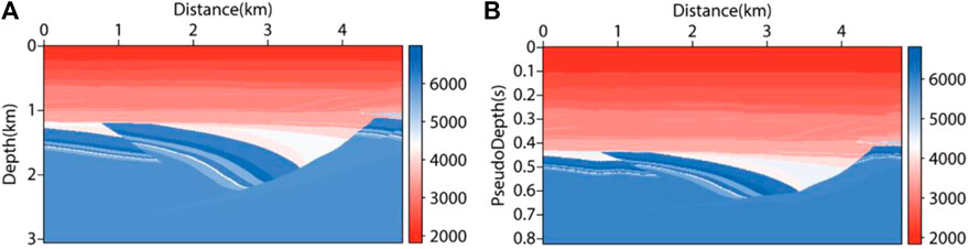
FIGURE 7. SL velocity field model. (A) real velocity field; (B) velocity field transformed into pseudo-depth domain.

The shot records obtained by forward modeling are shown in Figure 8. Figure 8A is the results of forward modeling in the depth domain; Figure 8B is the results of forward modeling in the pseudo-depth domain. Comparing the results of the two methods, the difference is subtle. In order to compare the difference in detail, a single trace comparison of two shot records was carried out. Single trace signals at x=2000m and x=4000 m were extracted, as shown in Figures 8C, D, respectively. It can be seen that the results of the two methods coincided well with each other, except for a slight difference in amplitude. Therefore, in the later numerical test, the pseudo-depth domain method could be used for seismic wavefield imaging. In this paper, preserved shot records were used to construct the receiver point wavefield by reverse extension, and the smooth velocity field in the depth domain or the pseudo-depth domain was used as the source wavefield by forward extension. The RTM imaging conditions mentioned above were used for migration imaging.

FIGURE 8

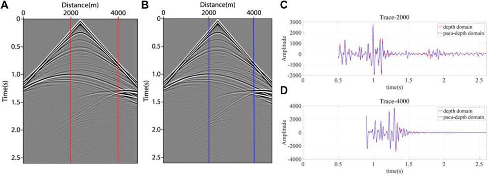
FIGURE 8. Single trace signal extract at the same location in different shot records. (A) depth domain method; (B) pseudo-depth domain method; (C) single trace signal located at 2000m; (D) single trace signal located at 4000 m.

The calculation time and memory consumption results of the single shot records obtained by the two methods in CPU were compared, which are shown in Table 1. In the process of forward modeling, the pseudo-depth domain method could improve calculation efficiency and reduce occupied memory, which saved about 22% of the calculation cost and 34% of the memory occupied separately.

TABLE 1

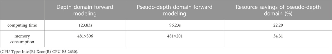
TABLE 1. Comparison of calculation efficiency and memory consumption from depth domain acoustic isotropy forward method and pseudo-depth domain forward method under CPU.

3.3 RTM imaging results in different method

This part mainly displays the imaging results of acoustic isotropy RTM, VTI RTM, and VTI PDRTM. Firstly, we established three groups of models with different characteristics for numerical simulation to verify the applicability and accuracy of imaging methods under different structures. Secondly, a set of land field data was used to reflect the application result of this method. Thirdly, according to the test time and memory usage of the model and field data, the advantages of our method were analyzed.

The smooth velocity field in Figure 9 was used to simulate the velocity field obtained by tomography or velocity analysis in practice. We used accurate forward modeling results of the velocity field as observation shot records. Among them, the calculation of vertical travel time and the transformation in pseudo-depth domain were carried out based on the smooth velocity field. The delta and epsilon parameter fields of the VTI medium were obtained by using the empirical equations mentioned above (as shown in Figures 9E–G). During the testing process, VTI parameters also needed to be transformed into the pseudo-depth domain. In the later research of this paper the VTI parameter fields were all obtained by empirical equations, and there was no difference in the structure shape with the velocity field, but only in the numerical value and physical meaning. Therefore, the related model test in VTI media mentioned in the later research of this paper no longer showed the anisotropic parameter field. For the migration of the SL model, the shot point and receiver point were set near the surface. The source adopted a 30 Hz Ricker wavelet. The target area size was 4810m×3060m, and the area size was 4810m×2010m after transforming to the pseudo-depth domain. In total, 121 shots were arranged, with a shot distance of 40 m. The receiver points adopted the mode of full receiving, with a maximum sampling time of 4s and a sampling interval of 0.6 ms. RTM imaging theory was used to SL model in the depth domain and the pseudo-depth domain, and the imaging results were displayed in the same condition. By comparing Figure 10A with Figure 10B, it can be seen that VTI RTM can depict the horizon more accurately, and the imaging results are clearer and more continuous. In the VTI medium, by comparing the imaging results of the depth domain method, the pseudo-depth domain method could achieve high-quality imaging sections and enhance the events energy of mid deep imaging. In Figures 10C, E, the x-direction and z-direction imaging profiles of the VTI medium in the pseudo-depth domain are given. After comparison, there was not much difference between them, so only the x-direction imaging profile was given in the following research of this paper..

FIGURE 9

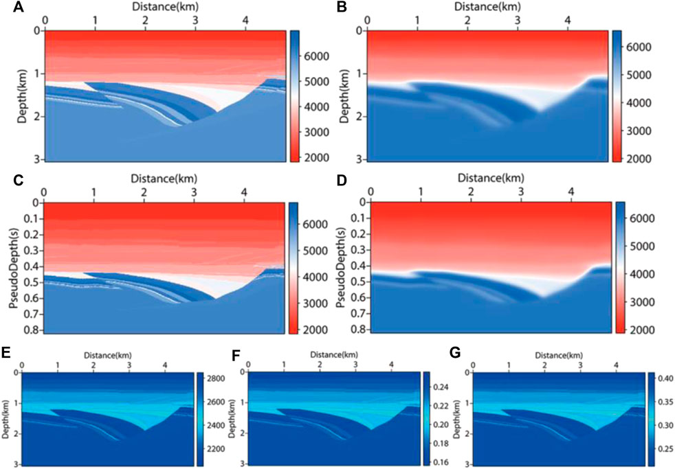
FIGURE 9. VTI parameter field of SL model. (A) depth domain true velocity field; (B) depth domain migration velocity field; (C) pseudo-depth domain true velocity field; (D) pseudo-depth domain migration velocity field; (E) density (𝛒) field; (F) delta (𝛅) field; (G) epsilon (𝛆) field.

FIGURE 10

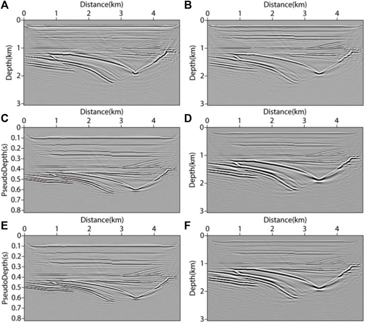
FIGURE 10. Migration results of SL model. (A) acoustic isotropy RTM method; (B) x-direction imaging results of VTI-RTM method in depth domain; (C) x-direction imaging results of VTI-PDRTM method; (D) inverse transform (C) to x-direction imaging results in depth domain; (E) z-direction imaging results of VTI-PDRTM method; (F) inverse transform (E) to z-direction imaging results in depth domain.

The pseudo-depth domain method mainly performs coordinate transformation in the vertical direction. To verify the adaptability of the pseudo-depth domain method in the long offset layered structure, we built a velocity model based on marine data (as shown in Figure 11). The size of the model area was 19650m × 2010m, with a grid spacing of 10 m. The top layer was the water layer with a velocity of 2000m/s, the shot point was placed 10 m away from the surface and the receiver was set on the surface. The main frequency of the source was 30 Hz. In total, 196 shots were placed with an interval of 100 m. The maximum sampling time was 6.336s, with a sampling interval of 0.6 ms. The region transformed to the pseudo-depth domain was 19650m×1410 m (as shown in Figure 11C). Figures 11B, D are smooth velocity fields, as the input migration velocity fields were used to simulate the velocity fields processed by velocity analysis and other methods. The imaging results after migration are shown in Figure 12. From Figures 12A, C, it can be seen that the RTM results of the depth domain and pseudo-depth domain in VTI media have little difference, the imaging quality is relatively good, and the layered structure can be clearly described from the inaccurate migration velocity. By comparing Figure 12A with Figure 12B, in the imaging of long offset layered strata, imaging artifacts will exist between migration result layers if vertical anisotropy is not considered, which negatively influence the imaging result ability to converge to the true position accurately. At the position of the black arrow in Figure 11 and Figure 12, there was some structural distortion in the velocity field and imaging results after the transformation to the pseudo-depth domain. This distortion could be eliminated after transforming back to the depth domain. The numerical simulation reflected that the pseudo-depth domain method has good adaptability for seafloor data and can get good imaging results.

FIGURE 11

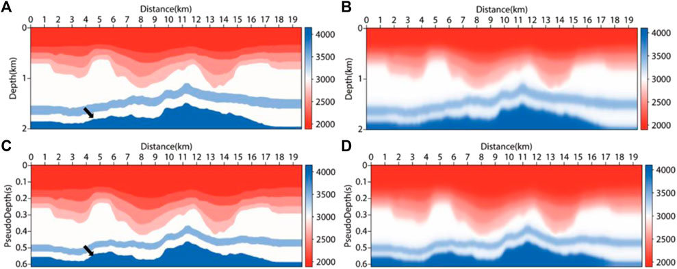
FIGURE 11. Velocity field of seafloor model. (A) depth domain true velocity field; (B) depth domain migration velocity field; (C) pseudo-depth domain true velocity field; (D) pseudo-depth domain migration velocity field.

FIGURE 12

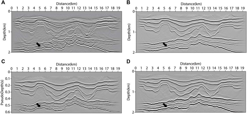
FIGURE 12. Migration results of seafloor model under GPU acceleration strategy. (A) acoustic isotropy RTM method; (B) VTI-RTM method in depth domain; (C) VTI-PDRTM method in pseudo-depth domain; (D) VTI-PDRTM method transformed back to the depth domain.

In addition, to verify that the pseudo-depth domain method can be applicable in more complex structural migration, and to further clarify that the inverse transformation after migration can eliminate the structural distortion caused by coordinate mapping, a more complex overthrust structure was selected as the test object. Similarly, the velocity field of the research target is shown in Figure 13. The test area was 8340m×5000m; 166 shots were placed in total, with the shot interval of 5 m and grid spacing of 10 m, and there are 834 receivers on the surface with spacing of 10 m. The maximum sampling time was 4.3s, and the sampling time interval was 0.3 ms. The results of migration are as shown in Figure 14. It can be seen from the black arrows of Figures 14A, B that the results obtained by RTM are clearer when VTI parameters are considered. The black arrow area in Figure 14B is cleaner and has a higher resolution than Figure 14A. Similar to the long offset seafloor model, in Figure 13 and Figure 14, it can be seen that structural deformation occurs in the pseudo-depth domain at the position of the yellow arrows. After the inverse transformation of the imaging results, the deformation was almost eliminated, as the yellow arrows show in Figure 14D. By comparing Figure 14B with Figure 14D, it can be found that, at the red arrows, the VTI PDRTM improves the structural imaging details at the locations where the VTI RTM is difficult to image. In complex constructions, the pseudo-depth domain method can get satisfactory imaging results.

FIGURE 13

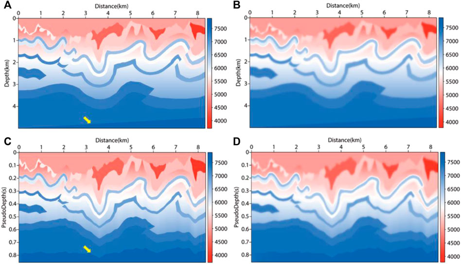
FIGURE 13. Velocity field of complex overthrust. (A) true velocity field in depth domain; (B) migration velocity field in depth domain; (C) true velocity field in pseudo-depth domain; (D) migration velocity field in pseudo-depth domain.

FIGURE 14

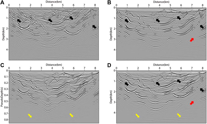
FIGURE 14. Migration results of complex overthrust model under GPU acceleration strategy. (A) acoustic isotropy RTM method; (B) VTI-RTM method in depth domain; (C) VTI-PDRTM method in pseudo-depth domain; (D) VTI-PDRTM method transformed back to the depth domain.

Next, we used the land field data set to compare the results of various migration methods. There were 204 shots of land field data used for migration, 60 seismic traces for each shot, and the shot spacing and receiver spacing were both 50 m. The migration parameter field was shown in Figures 15A, C, D, with a grid number of 1056 × 510 and a space sampling interval of 12.5 m. The time sampling interval was 1 ms, with a maximum sampling duration of 6s. The source wavelet adopted a 30 Hz Ricker wavelet. The shot point and receiver point of each shot were located 12.5 m away from the surface. After the velocity field was transformed into the pseudo-depth domain, the number of grids became 1056 × 357, as shown in Figure 15B. The seismic records of 100–105 shots extracted from the shot set in which the direct wave had been cut off are shown in Figure 16. The final imaging results are shown in Figure 17. Figures 17A–C are the imaging sections of RTM, VTI RTM, and VTI PDRTM, respectively. Figure 17D shows the result of transforming back to the depth domain. It can be seen from the comparison that the migration results in Figures 17B, D are more balanced in energy, more continuous in events and clearer in structure description.

FIGURE 15

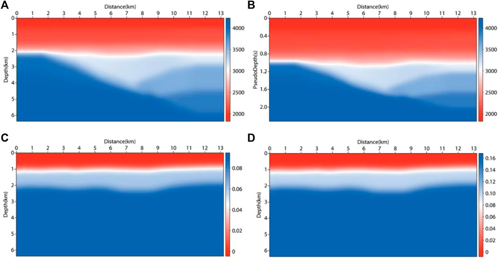
FIGURE 15. Migration model for the land field data set. (A) velocity field; (B) migration velocity field transformed to pseudo-depth domain; (C) delta (𝛅) field; (D) epsilon (𝛆) field.

FIGURE 16

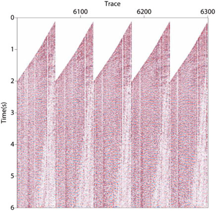
FIGURE 16. 100–105th shot records extracted from the land field data set.

FIGURE 17

FIGURE 17. Migration results of the land field data set. (A) acoustic isotropy RTM method; (B) VTI-RTM method in depth domain; (C) VTI-PDRTM method in pseudo-depth domain; (D) VTI-PDRTM method transformed back to the depth domain.

In order to make the comparison more intuitive, we selected three imaging regions at the same position for magnification in the migration results obtained by each method, as shown in Figure 18. It can be seen from Figures 18A–C, which were selected from the left red solid line box in Figure 17, that Figures 18B, C describe the horizon more clearly after considering anisotropy. Meanwhile, the pseudo-depth domain method in Figure 18C was better than the depth domain method in depicting faults (as shown by the red arrow). For the middle red solid box selected in Figure 17, the enlarged migration results also show that the migration results were more continuous in events after taking VTI parameters into account (as shown by the black arrows in Figures 18D–F). Regarding the right red solid box selected in Figure 17, at the red arrows in Figures 18G–I, the acoustic isotropic RTM could not image the undulating layer, while VTI RTM and VTI PDRTM could clearly depict the structure. In summary, after the migration processing of model and actual land data, VTI PDRTM and VTI RTM had almost the same imaging accuracy, with VTI PDRTM being better at characterizing some faults and minor structures. Then, we compared the calculation time and memory usage of various methods in respective tests.

FIGURE 18

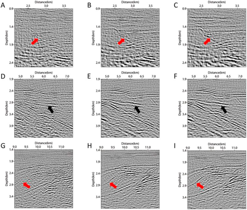
FIGURE 18. Enlarged imaging results corresponding to the red solid line boxes in Figure 17. Migration results of left solid line box using (A) RTM, (B) VTI RTM, (C) VTI PDRTM, respectively; migration results of middle solid line box using (D) RTM, (E) VTI RTM, (F) VTI PDRTM, respectively; migration results of right solid line box using (G) RTM, (H) VTI RTM, (I) VTI PDRTM, respectively.

As shown in Table 2, this paper gives the calculation efficiency and memory consumption of each region in RTM. It can be seen that VTI-RTM using GPU parallel acceleration strategy simulation could save about 70% of the computing cost compared with the CPU. Under the same conditions, the pseudo-depth domain method could reduce memory consumption by 30% and calculation time by 10–30%.

TABLE 2

TABLE 2. The calculation efficiency and memory consumption of different migration methods under the same calculation parameters.

4 Discussion

The pseudo-depth domain method redivided the grids calculated by the wave equations into one-way vertical travel time grids according to the smooth migration velocity. This method reduced the waste of computing resources, and to a certain extent, eliminated the velocity wavelength mapping ambiguity caused by the forced division of the vertical spatial grid. The purpose of our research on pseudo-depth domain RTM imaging in VTI media was to achieve a breakthrough, which anticipated more accuracy and efficiency in wave equations imaging of vertically anisotropic multi-layer geological targets. We analyzed the results in the following three aspects. First of all, the pseudo shear wave suppression in VTI acoustic approximate equations forward modeling was declared. In the next part, the comparison of forward modeling accuracy and calculation amount between the depth domain method and the pseudo-depth domain method was discussed. Furthermore, the simulated results of various RTM methods under different models were analyzed.

In this paper, the VTI wave equations were simplified by assuming that the shear wave was zero. The advantage of this method was that the wavefield was simple to realize, but would inevitably introduce low-speed and low amplitude pseudo shear wave interference, as shown in Figure 5B and Figure 6B in Section 3.1. If it was not suppressed, the accuracy of anisotropic media imaging and velocity modeling would be greatly affected, resulting in false imaging. Therefore, many scholars have done a lot of research on suppressing pseudo shear wave interference (Alkhalifah, 1998; Grechka et al., 2004; Duveneck et al., 2008; Zhang et al., 2009; Xu and Zhou, 2014). In our study, the method of loading source loop was used to suppress pseudo shear wave interference, which was a simple and effective method (such as Figure 5C; Figure 6C), and enough to meet the requirements of the following migration. The estimation of anisotropic parameters impacted VTI media migration. When the error exceeded 30%, the layers imaging would focus on the wrong position, which affected the subsequent interpretation (Moussavi Alashloo et al., 2016). Therefore, we used empirical formulas to calculate the anisotropic parameters, considering that the impact of the estimated value on the migration results could avoid the absurd values of the anisotropic parameters.

The basis of RTM is forward modeling. Both source wavefield forward extension and receive point wavefield reverse extension are forward simulation processes. In real production, only seismic records can be obtained. It is necessary to compare and analyze the forward process of the pseudo-depth domain and the depth domain. Only when the simulation results of the pseudo-depth domain are almost equal to the conventional ones, is it meaningful to use the pseudo-depth domain method in imaging. Therefore, it is very important to discuss whether the forward process is accurate in the pseudo-depth domain. In Section 3.2, the forward process using the pseudo-depth domain method and traditional finite difference method was simulated. The single shot records at the same observation system were given, as shown in Figure 8. For the convenience of analysis, this paper extracted two single trace records at different positions for amplification and comparison, as shown in Figure 8. Comparing the results of the two methods, it was obvious that the single trace signal obtained by the pseudo-depth domain method was well fit with the conventional method in amplitude and travel time. There were some differences between them in a few positions. The reason was the velocity field in the pseudo-depth domain was converted to approximate maximum vertical travel time by interpolation, which inevitably introduced data truncation errors. In the process of RTM, preprocessing and velocity modeling could not provide an accurate velocity field. Therefore, when the velocity field was smooth and mapped to pseudo-depth domain, the small error caused by data truncation could be ignored. In the last part of this section, we compared the computational efficiency and memory consumption of the two methods, as shown in Table 1. The pseudo-depth domain method could improve computational efficiency and reduce memory consumption, because it reduced about one-third of the grids after coordinate mapping. After a number of tests, we found that the reduced number of grid points should be controlled to between 30% and 40% in pseudo-depth domain mapping, otherwise it caused huge data distortion.

The effectiveness of the VTI PDRTM method was verified. For different structures, the RTM comparison tests of different methods in VTI media were carried out. In Section 3.3, three groups of different constructs were tested to make the results more reliable. We used an accurate model to do forward modeling with the acoustic isotropy finite difference method, which generated the shot records to construct the wavefield of the receiver point. At the same time, the true model was smoothed by the migration velocity field obtained after preprocessing or velocity modeling, which was used to construct the source wavefield. By comparing VTI RTM with acoustic isotropic RTM, the migration results of the three models and the field data were greatly improved, especially in terms of eliminating imaging artifacts, equalizing energy, and making the event more continuous (as shown by the black arrow in Figure 14). Pseudo-depth domain mapping of velocity field causing structural distortion was inevitable, but this effect could be eliminated by inverse transformation, as shown by the black arrow in Figure 12 and the yellow arrow in Figure 14. Our test results showed that the reduction of vertical grid points to within 30%–40% can ensure the data fidelity; that is, the structural distortion could be eliminated by inverse transformation. As shown by the yellow arrow in Figure 14D, most of the migration results were restored to the true position by inverse transformation. But the geological targets were imaged in the pseudo-depth domain, which could not image some deformed positions with large dip angles due to the accumulation of errors. When the migration profile was transformed back to the depth domain, layer discontinuity was caused. Through model testing, we found it was difficult to quantitatively define what kind of structure would cause this cumulative error. Therefore, this also became a research difficulty of the pseudo-depth domain method, which needs further research. In the land field data testing, because the migration velocity field of the land data used was relatively smooth, a more balanced and clean migration profile was obtained in the VTI PDRTM method. The fault location was more clearly depicted as shown in Figures 18A–C, which reflected the insensitivity of the pseudo-depth domain method to initial velocity.

In addition, we also compared the calculation time with memory consumption of each construction, as shown in Table 2. For different structures, the pseudo-depth domain method could ensure imaging accuracy while, at the same time, improve computational efficiency by 10%–30%, and save about 30% of the memory occupied. This was valuable for RTM, especially for deep or ultra-deep targets in vertical sense. However, saved calculation time was not linear with saved storage space, the reason being that the difference of the forward wavefield time sampling points led to inconsistencies between the CPU and GPU transmission time of each model. At the same time, under our method which combined GPU parallel and pseudo-depth domain strategies, the efficiency could be improved by about five times.

5 Conclusion

In this study, the GPU parallel strategy based PDRTM method under VTI media was developed. The pseudo-depth domain wave equations and their discrete forms for homogeneous media and VTI media were derived. By mapping coordinates to the pseudo-depth domain, this strategy can effectively save 10%–30% of computing time and 25%–30% of memory consumption on the premise of ensuring imaging accuracy. At the same time, GPU collaborative computing technology can save about 70% of the computing time and greatly improve efficiency. By introducing the method to VTI media, the migration results of complex structures are more reasonable than those of isotropy media. A deep complex structure imaging method needs to be developed urgently, which requires a huge amount of calculation. The developed pseudo-depth domain anisotropic imaging strategy in this paper provides a solution to reduce the amount of calculation and memory occupation. Although the GPU parallel acceleration PDRTM method can image in simple and complex structures effectively, some areas where near traces have dramatic changes, leading to accumulated errors in one-way vertical travel time, need further discussion in the future.

Data availability statement

The original contributions presented in the study are included in the article/supplementary material, further inquiries can be directed to the corresponding author.

Author contributions

ZX deduced the equations, carried out numerical simulation and wrote the manuscript; ZX and JZ cooperated to complete the preparation and debugging of the program; HJ and LZ gave writing and theoretical guidance; LQ provided basic ideas on the theory and programming of pseudo-depth domain; all authors have contributed to this paper and agree with the submission.

Funding

This study was co-funded by the National Key Research and Development Program of China (2019YFC0605503), the National Natural Science Foundation Project (41821002, 41922028, 41874149), and the major science and technology special project of CNPC (ZD2019-183-003).

Acknowledgments

The authors thank all members of the seismic inversion and imaging group of China University of Petroleum (East China) for their comments and discussions. The authors also thank the reviewers and the editorial department for their constructive and thoughtful comments and suggestions, which greatly improved the quality of this study.

Conflict of interest

Author JZ was employed by China Oilfield Services Limited. Author LQ was employed by Sinopec Zhongyuan Oilfield.

The remaining authors declare that the research was conducted in the absence of any commercial or financial relationships that could be construed as a potential conflict of interest.

Publisher’s note

All claims expressed in this article are solely those of the authors and do not necessarily represent those of their affiliated organizations, or those of the publisher, the editors and the reviewers. Any product that may be evaluated in this article, or claim that may be made by its manufacturer, is not guaranteed or endorsed by the publisher.

References

Alkhalifah, T. (1998). Acoustic approximations for processing in transversely isotropic media. Geophysics 63, 623–631. doi:10.1190/1.1444361

CrossRef Full Text | Google Scholar

Alkhalifah, T. (2003). Tau migration and velocity analysis: Theory and synthetic examples. Geophysics 68, 1331–1339. doi:10.1190/1.1598126

CrossRef Full Text | Google Scholar

Alkhalifah, T., Fomel, S., and Biondi, B. (2001). The space–time domain: Theory and modelling for anisotropic media. Geophys. J. Int. 144, 105–113. doi:10.1046/j.1365-246x.2001.00300.x

CrossRef Full Text | Google Scholar

Baysal, E., Kosloff, D. D., and Sherwood, J. W. C. (1983). Reverse time migration. Geophysics 48, 1514–1524. doi:10.1190/1.1441434

CrossRef Full Text | Google Scholar

Chang, W., and McMechan, G. A. (1986). Reverse-time migration of offset vertical seismic profiling data using the excitation-time imaging condition. Geophysics 51, 67–84. doi:10.1190/1.1442041

CrossRef Full Text | Google Scholar

Chang, W., and McMechan, G. A. (1987). Elastic reverse-time migration. Geophysics 52, 1365–1375. doi:10.1190/1.1442249

CrossRef Full Text | Google Scholar

Chang, W., and McMechan, G. A. (1994). 3-d elastic prestack, reverse-time depth migration. Geophysics 59, 597–609. doi:10.1190/1.1443620

CrossRef Full Text | Google Scholar

Claerbout, J. (1971). Toward a unified theory of reflector mapping. Geophysics 36, 467–481. doi:10.1190/1.1440185

CrossRef Full Text | Google Scholar

Dai, W., Fowler, P., and Schuster, G. T. (2012). Multi-source least-squares reverse time migration. Geophys. Prospect. 60, 681–695. doi:10.1111/j.1365-2478.2012.01092.x

CrossRef Full Text | Google Scholar

Du, Q., Zhu, Y., and Ba, J. (2012). Polarity reversal correction for elastic reverse time migration. Geophysics 77, S31–S41. doi:10.1190/geo2011-0348.1

CrossRef Full Text | Google Scholar

Duveneck, E., Milcik, P., Bakker, P. M., and Perkins, C. (2008). “Acoustic vti wave equations and their application for anisotropic reverse-time migration,” in SEG las vegas 2008 annual meeting (Las Vegas: SEG Library). doi:10.1190/1.3059320

CrossRef Full Text | Google Scholar

Foltinek, D., Eaton, D., Mahovsky, J., Moghaddam, P., and McGarry, R. (2009). “Industrial-scale reverse time migration on gpu hardware,” in SEG houston 2009 international exposition and annual meeting (Houston: SEG Library). doi:10.1190/1.3255428

CrossRef Full Text | Google Scholar

Grechka, V., Zhang, L., and Rector, J. W. (2004). Shear waves in acoustic anisotropic media. Geophysics 69, 576–582. doi:10.1190/1.1707077

CrossRef Full Text | Google Scholar

Gu, B., Liu, Y., Ma, X., Li, Z., and Liang, G. (2015). A modified excitation amplitude imaging condition for prestack reverse time migration. Explor. Geophys. 46, 359–370. doi:10.1071/EG14039

CrossRef Full Text | Google Scholar

Hayashi, K., and Burns, D. R. (1999). “Variable grid finite-difference modeling including surface topography,” in SEG 1999 expanded abstracts. doi:10.1190/1.1821071

CrossRef Full Text | Google Scholar

Kaelin, B., and Guitton, A. (2006). “Imaging condition for reverse time migration,” in SEG/New orleans 2006 annual meeting. doi:10.1190/1.2370059

CrossRef Full Text | Google Scholar

Li, Q., Huang, J., and Li, Z. (2017). Cross-correlation least-squares reverse time migration in the pseudo-time domain. J. Geophys. Eng. 14, 841–851. doi:10.1088/1742-2140/aa6b33

CrossRef Full Text | Google Scholar

Ma, X., and Alkhalifah, T. (2013). Wavefield extrapolation in pseudodepth domain. Geophysics 78, S81–S91. doi:10.1190/geo2012-0237.1

CrossRef Full Text | Google Scholar

McMechan, G. A. (1983). Migration by extrapolation of time dependent boundary values. Geophys. Prospect. 31, 413–420. doi:10.1111/j.1365-2478.1983.tb01060.x

CrossRef Full Text | Google Scholar

Moussavi Alashloo, S. Y., Ghosh, D. P., Bashir, Y., and Wan Ismail, W. Y. (2016). Influence of error in estimating anisotropy parameters on vti depth imaging. Int. J. Geophys. 2016, 1–6. doi:10.1155/2016/2848750

CrossRef Full Text | Google Scholar

Mu, X., Huang, J., Yang, J., Guo, X., and Guo, Y. (2020a). Least-squares reverse time migration in tti media using a pure qp-wave equation. Geophysics 85, S199–S216. doi:10.1190/geo2019-0320.1

CrossRef Full Text | Google Scholar

Mu, X., Huang, J., Yong, P., Huang, J., Guo, X., Liu, D., et al. (2020b). Modeling of pure qp- and qsv-waves in tilted transversely isotropic media with the optimal quadratic approximation. Geophysics 85, C71–C89. doi:10.1190/geo2018-0460.1

CrossRef Full Text | Google Scholar

Nguyen, B. D., and McMechan, G. A. (2013). Excitation amplitude imaging condition for prestack reverse-time migration. Geophysics 78, S37–S46. doi:10.1190/geo2012-0079.1

CrossRef Full Text | Google Scholar

Plessix, R. É. (2013). A pseudo-time formulation for acoustic full waveform inversion. Geophys. J. Int. 192, 613–630. doi:10.1093/gji/ggs056

CrossRef Full Text | Google Scholar

Riley, K., and Hobson, M. (2006). Mathematical methods for physics and engineering. Cambridge: Cambridge University Press.

Google Scholar

Suh, S., Yeh, A., Wang, B., Cai, J., Yoon, K., and Li, Z. (2010). Cluster programming for reverse time migration. Lead. Edge 29, 94–97. doi:10.1190/1.3284058

CrossRef Full Text | Google Scholar

Sun, R., and McMechan, G. A. (1986). Pre-stack reverse-time migration for elastic waves with application to synthetic offset vertical seismic profiles. Proc. Ieee 74, 457–465. doi:10.1109/PROC.1986.13486

CrossRef Full Text | Google Scholar

Sun, X., Jia, Y., Zhang, M., Li, Q., and Li, Z. (2018). Least squares reverse-time migration in the pseudodepth domain and reservoir exploration. Appl. Geophys. 15, 234–239. doi:10.1007/s11770-018-0681-x

CrossRef Full Text | Google Scholar

Symes, W. W. (2007). Reverse time migration with optimal checkpointing. Geophysics 72, M213–M221. doi:10.1190/1.2742686

CrossRef Full Text | Google Scholar

Virieux, J. (1984). Sh-wave propagation in heterogeneous media: Velocity-stress finite-difference method. Geophysics 49, 1933–1942. doi:10.1190/1.1441605

CrossRef Full Text | Google Scholar

Virieux, J. (1986). P-Sv wave propagation in heterogeneous media: Velocity-stress finite-difference method. Geophysics 51, 889–901. doi:10.1190/1.1442147

CrossRef Full Text | Google Scholar

Wang, Z., Huang, J., Liu, D., Li, Z., Yong, P., and Yang, Z. (2019). 3d variable-grid full-waveform inversion on gpu. Petroleum Sci. 16, 1001–1014. doi:10.1007/s12182-019-00368-2

CrossRef Full Text | Google Scholar

Wang, Z., Huang, J., Li, Z., Liu, D., and Yong, P. (2020). An efficient and accurate finite-difference operator using adaptively discretized grids and its application for 3d least-squares reverse-time migration. Arabian J. Geosciences 13, 480. doi:10.1007/s12517-020-05417-4

CrossRef Full Text | Google Scholar

Whitmore, N. D. (1983). Iterative depth migration by backward time propagation. Las Vegas: SEG Technical Program Expanded Abstracts 1983. doi:10.1190/1.1893867

CrossRef Full Text | Google Scholar

Xu, S., and Zhou, H. (2014). Accurate simulations of pure quasi-p-waves in complex anisotropic media. Geophysics 79, T341–T348. doi:10.1190/geo2014-0242.1

CrossRef Full Text | Google Scholar

Yang, J., Zhu, H., McMechan, G. A., Zhang, H., and Zhao Yang, Z. Y. (2019). Elastic least-squares reverse time migration in vertical transverse isotropic media. Geophysics 84, S539–S553. doi:10.1190/geo2018-0887.1

CrossRef Full Text | Google Scholar

Yang, J., and Zhu, H. (2019). Viscoacoustic least-squares reverse time migration using a time-domain complex-valued wave equation. Geophysics 84, S479–S499. doi:10.1190/geo2018-0804.1

CrossRef Full Text | Google Scholar

Zhang, H. J., Zhan, G., and Zhang, Y. (2009). “Removing s-wave noise in tti reverse time migration,” in SEG houston 2009 international exposition and annual meeting. doi:10.1190/1.3255441

CrossRef Full Text | Google Scholar