Velocity changes after the 2021 MS 6.4 Yangbi earthquake based on passive image interferometry

An M_S 6.4 earthquake occurred in Yangbi, Yunan Province, China, on 21 May 2021. The epicenter was on the blind branch fault in the west of the Weixi–Qiaohou–Weishan fault, but no surface rupture was obvious. In the present study, the continuous vertical component of waveforms that were recorded in six nearby permanent stations was collected and the noise cross-correlation and autocorrelation techniques were utilized to investigate velocity changes that were induced by the Yangbi Earthquake. Velocity changes based on the single-station autocorrelation method reveal mainly coseismic declines, and a maximum of .09% was recorded in the EYA station. Results from the cross-correlation technique show both positive and negative velocity changes, and these lasted for approximately 3 months. The volumetric strain that was generated by the Yangbi Earthquake at a depth of 5 km exhibits an obvious four-quadrant distribution. Station pairs in the dilatation region (e.g., EYA–HEQ) mainly display a decrease in velocity, whereas those in the contraction region (e.g., BAS–TUS, TUS–YUL, and LUS–TUS) show an increase in velocity. Based on the depth sensitivity of scattered waves, velocity changes that were obtained using the noise cross-correlation involve the highest weight coefficients near the related two stations. Regarding stations of one station pair in different stress loading regions, the static stress of the station that is nearest to the epicenter exerted a greater impact on the velocity change. The observed velocity changes are likely attributed to a combination of near-surface physical damage and static stress changes. The validation of clock errors with magnitudes of seconds that were obtained using the noise cross-correlation and effects of these errors on measured velocity changes are also discussed.

1 Introduction

The state of stress and properties of the medium in a fault zone can change significantly during the nucleation and occurrence of an earthquake (Kanamori, 1994; Liu et al., 2014). Therefore, studies on changes in the medium are useful to understand the evolution and healing of faults, as well as the evolution of earthquake risk analysis. Seismologists have proposed the use of repeated earthquake data to characterize velocity perturbations in the crust because earthquakes, which originated from deep underground locations, reveal significant information of the source area (Poupinet et al., 1984; Peng and Ben-Zion, 2006). However, repeated earthquakes are spatiotemporally limited, and these are often associated with regions of high seismic activity. Artificial sources that produce similar waveforms are also useful for the monitoring of temporal changes in such media (Reasenberg and Aki, 1974; Vidale and Li, 2003; Wang et al., 2008). Su et al. (2022) reported coseismic velocity variations of .08%–.12% near the fault zone of the 2021 M_S 6.4 Yangbi Earthquake based on seismic wave signals that were generated using Binchuan Airgun. In the past decade, the passive monitoring of seismic velocity using interferometry increased significantly. This was utilized to monitor fault systems and landslides (Brenguier et al., 2008a; Liu et al., 2014; Liu et al., 2018; Boschelli et al., 2021; Huang et al., 2021; Le Breton et al., 2021), predict volcanic intrusions (Brenguier et al., 2008b; Liu et al., 2022), and explore changes in shallow groundwater (Clements and Denolle, 2018; Mao et al., 2022). These studies generally assumed that the coda part of noise cross-correlation functions travels a longer path that broadly samples the medium compared to direct waves, and is therefore more sensitive to small perturbations in the medium (Snieder et al., 2002; Sheng et al., 2021).

The methods that can be used to calculate the travel time shift δt between earthquake doublets can be divided into three categories: 1) Time-domain methods such as windowed cross correlation (Snieder et al., 2002), trace stretching (Sens-Schönfelder and Wegler, 2006; Obermann et al., 2016), and dynamic time warping (Meier et al., 2010); 2) Frequency-domain methods such as moving window cross spectrum (MWCS) (Poupinet et al., 1984; Liu et al., 2018); and 3) Wavelet-domain methods such as wavelet cross spectrum (Mao et al., 2020) and wavelet trace stretching (Yuan et al., 2021). Liu et al. (2010) compared and analyzed the advantages and disadvantages of four common methods and concluded that the MWCS performed better due to small measurement errors. Moreover, MWCS separates amplitude spectrum and phase spectrum before measurement, so it is less affected by the frequency of ambient noise (Zhan et al., 2013).

Mechanisms of velocity changes induced by earthquakes, such as static stress and pore pressure variations, as well as near-surface and fault zone physical damage remain controversial (Poupinet et al., 1984; Rubinstein and Beroza, 2004; Wegler et al., 2009; Sheng et al., 2021). On 21 May 2021, an M_S 6.4 earthquake (epicenter at 25.67°N and 99.87°E) occurred in Yangbi County in the west of Yunan province, China. The epicenter of the earthquake was on the blind branch fault in the west of the Weixi–Qiaohou–Weishan fault, and surveys revealed no obvious surface rupture (Li et al., 2021; Zhu et al., 2022). This was the strongest shallow earthquake in Yunnan in the past decade following the M_S 6.5 Ludian and M_S 6.6 Jinggu earthquakes (Zhang et al., 2021).

In the present study, continuous data that were recorded in six nearby permanent stations was collected and both the ambient noise cross-correlation and autocorrelation methods were utilized to characterize velocity changes induced by the Yangbi Earthquake. Unlike many previous cases, both positive and negative velocity changes were obtained by using cross-correlation method. Mechanisms involved in the velocity changes were then examined based on the distributions of sensitivity associated with scattered waves and the static stress field. We also found clock errors of up to 1 year and up to 1 s in the data recorded at the EYA and LUS stations, respectively. Effects of the clock errors on measured of velocity changes were then analyzed.

2 Data and method

2.1 Data

The M_S 6.4 Yangbi earthquake is located in western Yunnan, which is located in the southeast margin of Tibet Plateau (Figure 1). It is the Yangtze paraplatform and northwest Yunnan geosynclinals fold belt junction area, which has strong characteristics of structural tension since the Quaternary period (Huang et al., 2014). In the present study, the vertical component of continuous waveforms (100 Hz) that were recorded in six broadband stations that are located within approximately 100 km of the epicenter of the Yangbi Earthquake between January 2019 and December 2021 was utilized (Figure 1). The area hosting the hypocenter was adequately covered by ten station pairs, and the minimum, maximum, and average distances between these stations pairs are 52, 143, and 97 km, respectively.

FIGURE 1

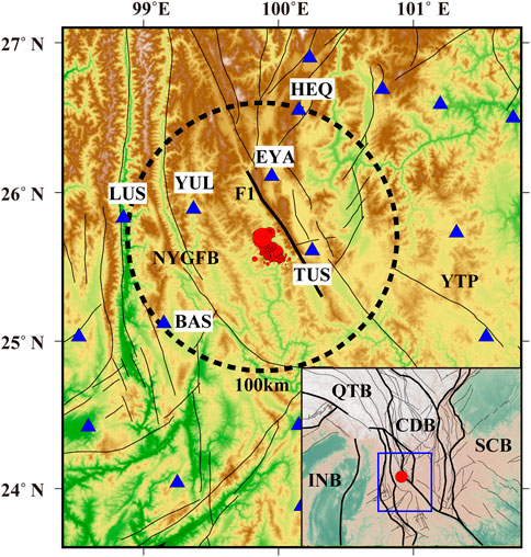
FIGURE 1. The tectonic background of the Yangbi earthquake sequence. Six broadband stations are located in the black circle area, which within approximately 100 km of the epicenter. F1 denotes the Weixi-Qiaohou-Weishan fault. The abbreviations denote the tectonic units. NYGFB, Northwest Yunnan geosynclinal fold belt; YTP, Yangtze Paraplatform; CDB, Chuandian Block; QTB, Qiangtang Block; SCB, South China Block; INB, Indian Block. The inset denotes the location of the research area. The red dot denotes the mainshock in both the main figure and the inset.

2.2 Green’s function retrieval

The data preprocessing procedure that was utilized in the present study was described in Liu et al. (2014). Raw seismic data were partitioned into 1-day intervals and the vertical component data were then resampled at 10 Hz to improve computational efficiency. Temporal normalization and spectrum whitening in the 1–20 s range were applied to each segment to minimize earthquakes effects. Reference cross-correlation functions (CCFs) for station pairs were obtained via the stacking of CCFs covering the period from 1 January 2019, to 21 April 2021 (a month preceding the Yangbi Earthquake). To improve the signal-to-noise ratio of daily CCFs, these were derived through the stacking of CCFs for 61 d, which included 30 d before and after a target day. To prevent mixing of pre- and post-seismic signals, daily CCFs that were calculated for periods before and after the Yangbi Earthquake were stacked separately (Liu et al., 2014; Liu et al., 2022). For example, the daily CCF on 28 May 2021 is obtained from stacking only post-seismic daily CCFs from 22 May 2021 to 28 June 2021. Thus, the stacking days of daily CCFs is smaller than 61 d within a month before and after the main shock. Daily CCFs for the EYA–YUL station pair in the period band of 1–10 s from January 2019 to December 2021 are shown in Figure 2A, and clear surface and stable coda wave signals are obvious. Owing to the decrease of the coda wave coherence as the timelapse increases, the lapse window for the positive portion of CCFs was determined as 30–130 s after the arrival of Rayleigh waves in this period band (Supplementary Figure S1). The windows in the negative portion were symmetrical to that in the positive portion.

FIGURE 2

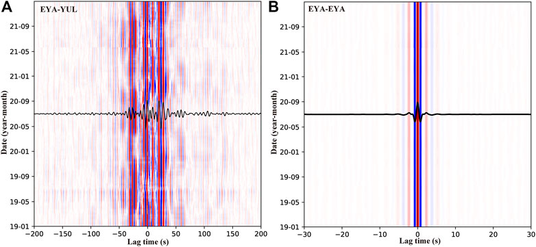
FIGURE 2. Daily CCFs for (A) EYA-YUL station pair in the period band of 1–10 s and (B) single station (EYA) in the period band of 1–3 s from January 2019 to December 2021. Waveforms in black represent reference CCFs, and red and blue correspondingly denote positive and negative.

To supplement station pairs near the epicenter, the single-station autocorrelation approach was also considered. Autocorrelation functions mainly reflect changes in the shallow crust near a station, and the associated flow processing is similar to that for the cross-correlation of a station pair. Figure 2B shows the autocorrelation functions for the EYA station using 1–3 s band-pass filter from January 2019 to December 2021. The lapse windows for the autocorrelation were determined as the fixed windows with range of ±(5–55) s.

2.3 Velocity change measurement using coda wave interferometry

Large to medium velocity perturbations can be directly obtained by measuring the relative traveltimes of the direct waves. Studies on the detection of small–medium changes as a function of time have focused on seismic coda waves. Coda waves, which are also known as multiply scattered waves, usually arrive later than direct waves. The later the arrival of scattered wave phases at the receiver, the longer the associated propagation paths and the higher the sensitivity to minor perturbations in a medium (Snieder et al., 2002).

Assuming that the change of relative seismic wave velocity (δv/v) is spatially homogeneous, the travel time shift δt between CCFs is proportional to the lapse time t and can be calculated as δv/v = −δt/t (Poupinet et al., 1984; Snieder et al., 2002). Therefore, the measurement of the travel time shift δt is very important for coda wave interferometry. In the present study, the MWCS method was utilized to measure the relative time shift between a reference CCFs that corresponds to the initial state, and a current CCFs that has encountered a velocity change in the medium. With the MWCS method, a series of overlapping time windows are defined in the coda wave, and the time shifts in these windows are estimated by means of the cross-spectrum method. The cross-spectrum X(f) between the reference CCFs and current CCFs is calculated as follows (Clarke et al., 2011):

$\mathrm{X}\left(f\right)=F_{ref}\left(f\right)\cdot F_{cur}^{*}\left(f\right)(1)$

where $F_{ref}$ and $F_{cur}$ are the Fourier-transformed segments of the reference and current CCFs. The asterisk denotes the complex conjugation and f is the frequency. $\mathrm{X}\left(f\right)$ can also be expressed by its amplitude $\left|\mathrm{X}\left(f\right)\right|$ and phase $e^{i\varphi \left(f\right)}$. If the time-shift is constant in each window segment, $\mathrm{\varphi }$ is linearly proportional to f:

$\mathrm{\varphi }\left(f\right)=2\pi \delta tf(2)$

The time shift for each window segment is the slope and the associated error $e_m$ is caulcuated as

$e_m=\sqrt{{\displaystyle \sum }_j{\left(\frac{w_j{v}_j}{{\sum }_i{w}_i{v}_i^2}\right)}^2\frac{{\sum }_j{\left({\varphi }_j-m{v}_j\right)}^2}{N-1}}(3)$

where $w$ are weights, m is the slope of $\varphi$, and $v$ are $2\pi f$.

After all time shifts δt are measured in the window segments in an interest range of lapse time, the relative time shift δt/t is estimated by a weighted linear regression passing through zero, and then δv/v can be obtained by −δt/t (Poupinet et al., 1984; Clarke et al., 2011). To evaluate the reliability and accuracy of the method, waveform modeling data that were reported in Yuan et al. (2021) were used, and the +.1% velocity perturbation that was determined in the model was correctly measured (Supplementary Figure S2).

Figure 3 shows an example of the relative time shift estimation using CCFs for the EYA–TUS station pair. Compared with the theoretical waveform in Supplementary Figure S2, CCFs of the EYA–TUS station pair produced a lower coherence and preserved the acausal signal. Regarding a 1–10 s period band and a station pair with distance of 62 km, the timelapse window is between 53 and 153 s and window segments are 18 s with a step of 1 s. Time shifts ($\delta \mathrm{t}$) between reference and daily CCFs can be measured in each window segments by using the MWCS, and the slope ($\delta \mathrm{t}/\mathrm{t}$) can then be estimated via a weighted linear regression of the time shifts.

FIGURE 3

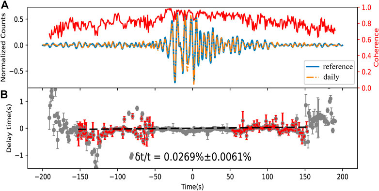
FIGURE 3. Example of a relative time shift ($\delta \mathrm{t}/\mathrm{t}$) that was estimated from CCFs in the period band of 1–10 s for the EYA–TUS station pair showing (A) waveforms of reference CCFs (blue) and daily CCFs for 1 April 2021 (yellow). The curve in red denotes the correlation coefficient. (B) The relative time shift ($\delta \mathrm{t}/\mathrm{t}$) for 1 April 2021. Circles containing error bars represent time shifts that were calculated in sliding windows, whereas the slope of the dash line in black was estimated using a weighted linear regression of all red time shifts.

3 Velocity changes caused by the Yangbi earthquake

Figure 4 shows continuous seismic velocity changes for the eight station pairs that cover the area of the epicenter of the Yangbi Earthquake. Coseismic velocity changes are observed in most station pairs, but unlike in many previous studies, velocity declines are evident in just three station pairs. Velocity changes of station pairs BAS-EYA, BAS-TUS, EYA-TUS, and LUS-TUS are relative stable and around the zero line before the main shock. The largest coseismic decrease is .06% for pair BAS-EYA, whereas the largest increasing is .14% for pair LUS–TUS that involves a path through the epicenter. These coseismic velocities are usually underestimated because of the long stacking days for the daily CCFs. Regardless of an increase or decrease in the coseismic velocity, the influence of the Yangbi Earthquake is evident for station pairs that display relatively stable results, such as the BAS–EYA, BAS–TUS, and LUS–TUS, and the influence last for approximately 3 months. Errors associated with the calculation of velocity changes are relatively high during the 1-month periods before and after the earthquake. These large errors are attributed to the reduction of stacking days because of the separation of stacking procedures of daily CCFs into those before and after the earthquake. Another reason is that because the Yangbi Earthquake is a typical foreshock–mainshock–aftershock type (Chen et al., 2022), the abundant foreshock and aftershock activities affect the stability of the empirical Green’s functions.

FIGURE 4

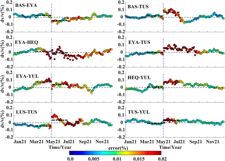
FIGURE 4. Continuous velocity changes obtained via the cross-correlation technique near the epicenter of the Yangbi Earthquake. The vertical dashed line in blue denotes the times of the earthquake, whereas the two thick dashed lines in black represent average values during the 2-month periods before and after the earthquake. The thin dashed line in black marks the zero levels, whereas dot colors highlight measurement errors, and the error scale is depicted.

Considering the average dv/v for the 2-month period preceding the earthquake as the reference value and that of the corresponding period after the earthquake minus the reference as the coseismic velocity change, a spatial distribution of coseismic velocity changes was obtained (Figure 5). Evidently, the Yangbi Earthquake mainly increased velocities in the study area. Station pairs of BAS-EYA, BAS-TUS, and EYA-TUS enclose the seismogenic fault and aftershock area. Coseismic velocity changes of pairs BAS-EYA and BAS-TUS, which across the fault zone, are −.07% and +.05%, whereas that of EYA-TUS on the east of the fault is +.06%. The relative velocity of the LUS–TUS station pair that involves a path through the epicenter increase by approximately .08%, but that of the TUS-YUL with a similar path increase slightly. Station pairs related to the TUS or YUL stations, which are in the near-field, are mainly characterized by an increase in velocity, whereas those involving the EYA station exhibit a decline.

FIGURE 5

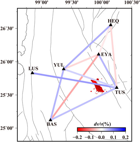
FIGURE 5. Spatial distribution of mean coseismic velocity changes. The mean coseismic velocity change is the difference between average velocity changes during the 2-month periods before and after the earthquake. Lines in blue indicate positive values, whereas those in red depict negative values.

Field surveys revealed that no obvious surface rupture was caused by the earthquake (Li et al., 2021; Zhu et al., 2022). According to simulations of strong ground motions, the peak ground acceleration exhibits a circular shape around the epicenter, and the ground motions beyond 60 km decay rapidly (Zhou et al., 2021). To evaluate perturbations of the Yangbi Earthquake on the shallow crust in the near-field, the single-station autocorrelation method was used to obtain the continuous velocity changes for single stations in the period band of 1–3 s (Figure 6). The results show that, excluding the LUS station, which is farthest from the epicenter, the other five stations exhibit a decline in the coseismic velocity. The highest decline of .09% was obtained from the EYA station, and these effects of the earthquake lasted for approximately 2–3 months. Data for coseismic velocity changes that were obtained using the noise cross-correlation and autocorrelation techniques are presented in Table 1.

FIGURE 6

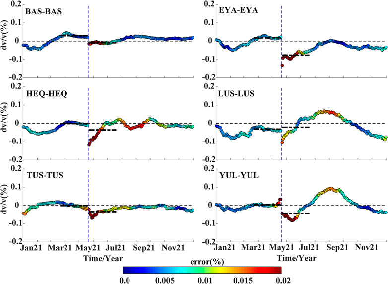
FIGURE 6. Continuous velocity changes near the epicenter of the Yangbi Earthquake that were derived using the autocorrelation technique. The vertical dashed line in blue denotes the time of the Yangbi Earthquake, whereas the two thick dashed lines in black are averages for the 2-month periods before and after the earthquake. The thin dashed line in black represents zero levels, whereas dot colors depict measurement errors, and the error scale is shown.

TABLE 1

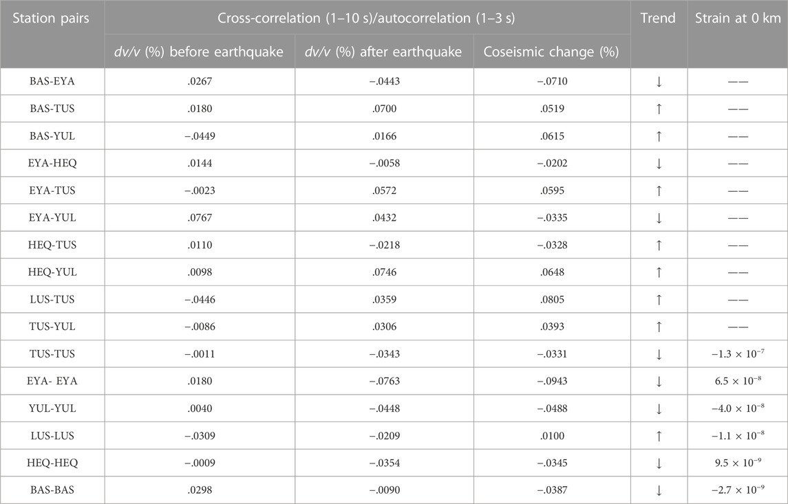
TABLE 1. Velocity changes caused by the Yangbi earthquake.

4 Discussion

There are four different mechanisms for velocity changes caused by earthquakes (Poupinet et al., 1984; Rubinstein and Beroza, 2004; Wegler et al., 2009; Boschelli et al., 2021; Sheng et al., 2021): 1) the change of the static stress results in positive and negative velocity changes; 2) the change of fluid content and pore pressure variations affects velocity; 3) the physical damage caused by fault motion; 4) near-surface physical damage caused by strong ground motion. Owing to the Yangbi Earthquake, excluding the LUS station (∼104 km from the epicenter), which showed a slight increase in velocity, autocorrelation analysis results for the other five stations revealed declines in the coseismic velocity. These decreases in velocities are mainly attributed to near-surface physical damage caused by the strong ground motion. Conversely, results from the noise cross-correlation analysis are difficult to explain. But first and foremost, the clock error or instrumental time shift is needed to be considered in using passive image interferometry (Liu et al., 2010).

4.1 Clock errors and their effects on velocity changes

Variations in spatial distributions of noise sources and the instrumental clock errors can independently affect the measurement of the travel time shift (Stehly et al., 2007). Clock errors can produce an overall shift in the entire cross-correlation time, thereby increasing traveltimes in the positive portion and decreasing traveltimes in the negative portion, and vice versa. Comparatively to the measurement of velocity changes in a medium, a direct arrival surface wave was used instead of a coda wave to measure instrumental clock errors. Clock errors that was measured from the surface wave using the noise cross-correlation technique can be expressed as follows (Stehly et al., 2007):

$\frac{\mathrm{\delta }\mathrm{\tau }\left(\mathrm{t}\right)+\mathrm{\delta }\mathrm{\tau }\left(-\mathrm{t}\right)}{2}=\mathrm{D}\left(\mathrm{t}\right)+\frac{\mathrm{\epsilon }\left(\mathrm{t}\right)+\mathrm{\epsilon }\left(-\mathrm{t}\right)}{2}(4)$

where $\mathrm{\delta }\mathrm{\tau }\left(\mathrm{t}\right)$ denotes the variation in the traveltime of the surface wave that is measured in the positive or negative portion. $\mathrm{D}\left(\mathrm{t}\right)$ is the time shift caused by instrumental clock errors, and $\mathrm{\epsilon }\left(\mathrm{t}\right)$ is the time shift associated with the spatial variation of noise sources. Therefore, clock errors can be estimated using Eq. 4 by assuming that $\mathrm{D}\left(\mathrm{t}\right)$ is greater than $\frac{\mathrm{\epsilon }\left(\mathrm{t}\right)+\mathrm{\epsilon }\left(-\mathrm{t}\right)}{2}$.

Following approaches that were advanced in Section 2.2 and Section 2.3, only the coda wave window was replaced with a surface wave window, that is, it starts 30 s before the surface wave time and ends 40 s after. Supplementary Figure S3 shows an example of clock errors that were estimated using data from the LUS–YUL station pair. The clock errors that were obtained on August 1 and October 20, for example, are .42 and −.04 s, respectively. The clock error on October 20 is less than one sampling rate, and thus, it can be considered as zero. Clock errors for these stations were evaluated for the period from 2019 to 2021, and results for station pairs with possible large clock errors are shown in Figure 7. The EYA station displays a clock drift of approximately −0.2 s throughout 2019, whereas LUS station exhibits a clock drift of −.6 s between July and August 2021. Considering that daily CCFs were obtained by stacking CCFs of 61 days, the estimated clock drifts are likely underestimated, in particular, the clock drifts from the LUS station may reach seconds.

FIGURE 7

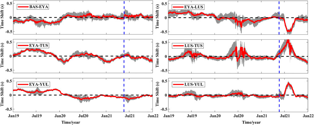
FIGURE 7. Clock errors for different station pairs between 2019 and 2021. The area shaded in gray represents the standard deviation, and this was used to highlight the calculation error. The vertical dashed line in blue denotes the time of the Yangbi Earthquake.

Two groups of teleseismic earthquakes that occurred in the Alaska Peninsula and the Philippines are selected to validate the clock drifts (Supplementary Tables S1, S2; Supplementary Figure S4). Differences in traveltimes of the phases between stations should essentially stable over time for nearby teleseismic earthquakes. But the reference arrivals of earthquakes on July 29 and 14 August 2021, were relatively early at the LUS station compared to that of other three earthquakes (Supplementary Figure S5). If the linear trend in Supplementary Figure S5B is eliminated, more intuitive reference arrivals relative to the distance from the epicenter can be obtained. Supplementary Figure S6A demonstrates that arrivals of earthquakes on July 29 and 14 August 2021, at the LUS station significantly differ from those of the other three earthquakes, and the drift is −1 s. Arrivals of all earthquakes at the other four stations do not show any obvious drift between 22 July 2020, and 11 October 2021. In addition, arrivals of earthquakes at the EYA station in 2019 slightly differ from those of the other three events, and the drift is −.3 s (Supplementary Figure S6B).

Considering the LUS–YUL station pair as an example, the velocity change that was calculated using the least squares fitting MWCS method is less than .02% for a clock error of 1 s (Figure 8). This minimal impact is probably because the slope of dt/t based on the MWCS method is unaffected by such an overall time drift of the cross-correlation time. However, a large clock error reduces the correlation between the reference and daily CCFs, and this affects subsequent calculations.

FIGURE 8

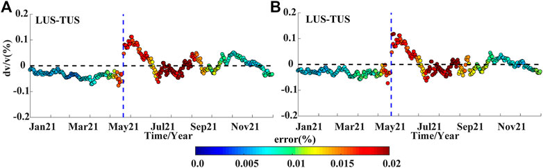
FIGURE 8. Velocity change measurements involving (A) no clock error correction and (B) with a clock error correction.

4.2 Static stress changes caused by the Yangbi earthquake

Positive and negative velocities linked to earthquakes may correspond to regions of increased and decreased stress, respectively (Rubinstein and Beroza, 2004). To explain observations from the noise cross-correlation, static stress changes caused by the earthquake were calculated using Coulomb 3.0 (Lin and Stein, 2004). The static slip distribution of the Yangbi Earthquake provided by Xu Zhang was utilized (https://www.cea.igp.ac.cn/kydt/278248.html, see Supplementary Figure S7), whereas the Poisson’s ratio and shear modulus were set to .25 and 32 GPa, respectively. The calculated volumetric strains caused by fault slips at a depth of 5 km exhibit an obvious four-quadrant distribution (Figure 9). The EYA and HEQ stations are in the dilatation region, where a decrease in velocity is anticipated, in fact, the velocity changes for the EYA–HEQ station pair decreased by .02%. The other four stations fall within the contraction region, where a velocity increase is expected, in fact, velocity changes for the BAS–TUS, TUS–YUL, and LUS–TUS station pairs corresponding increased by .05%, .04%, and .08%. However, how to decide if two stations are in different strain regions. For example, the velocity changes for the EYA–TUS station pair increased by .06%, whereas that for the EYA-YUL pair decreased by .03%. Therefore, an analysis of the spatial sensitivity distribution of coda waves is necessary.

FIGURE 9

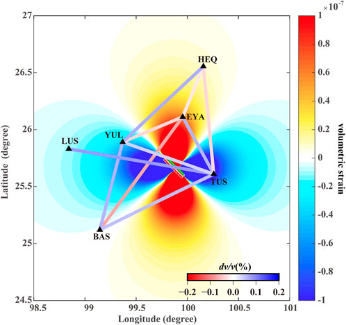
FIGURE 9. Volumetric strain changes caused by the Yangbi Earthquake at a depth of 5 km. The region of positive strain is dilatation and shown in red. Blue areas denote contraction. Lines connecting two stations correspond to the noise cross-correlation between the stations, and their values are presented in Table 1.

4.3 Depth sensitivity of coda waves

Based on numerical simulations of seismic waves in 2D and 3D heterogeneous elastic media, Obermann et al. (2013) suggested that the sensitivity of coda waves can be modeled as a linear combination of the sensitivities of body and surface waves. They indicated that early coda waves are dominated by fundamental surface waves, which mainly reflect shallow perturbations, whereas later coda waves are dominated by body waves. In the present study, the timelapse windows for CCFs were determined as 30–130 s after the arrivals of Rayleigh waves, and this contained sufficiently long signals. The sensitivity kernel that is expressed as follows can be used (Pacheco and Snieder, 2005):

$\mathrm{K}\left(\mathbf{S},\mathbf{R},{\mathbf{r}}_0,\mathrm{t}\right)=\frac{1}{p\left(\mathbf{S},\mathbf{R},\mathrm{t}\right)}\underset{0}{\overset{t}{{\displaystyle \int }}}p\left(\mathbf{S},{\mathbf{r}}_0,{\mathrm{t}}^{\prime }\right)p\left({\mathbf{r}}_0,\mathbf{R},\mathrm{t}-{\mathrm{t}}^{\prime }\right)d{t}^{\prime }(5)$

where S and R are the positions of the source and receiver, respectively; r₀ is the position of the local velocity variation; t is the center timelapse for doublet analysis; and p (s, r, t) is the probability that the wave has traveled from s to r during t. This probability can be approximated using the full-space solution of the diffusion equation, which is expressed as follows (Mao et al., 2019):

$\mathrm{p}\left(\mathbf{s},\mathbf{r},\mathrm{t}\right)=\frac{1}{(4\pi D{t)}^{3/2}}{e}^{\frac{-\Vert s-{r\Vert }^2}{4Dt}}(6)$

where D is the diffusion constant. The multiply scattered waves that propagate in 3 dimensions can be described by D:

$\mathrm{D}=\frac{C_E\ast l^{\ast }}{3}(7)$

where C_E is the energy velocity and l* is the scattering mean free path. Considering that S waves account for most of the energy in coda waves, a ratio of 9:1 was used to calculate C_E: $\frac{1}{C_E}=\frac{0.89}{Vs}+\frac{0.11}{Vp}$ (Obermann et al., 2016). Therefore, the key to determine the sensitivity kernel is to estimate the scattering mean free path l*. In general, at a larger scale (e.g., crustal) the mean free path is fairly constant relative to the frequency, but this may not be applicable at local scales. Chaput et al. (2015) estimated that the scattering mean free path for the Erebus volcano in Antarctica at 1.5 Hz is ∼2 km, and values slowly decreased as the frequency increased. Data for the scattering mean free path for the Yangbi area are scant, but theoretically values that involve 5%–10% heterogeneity are in the range of 2–10 km (Obermann et al., 2013). Here, l* = 5 km was considered in the period band of 1–10 s for analysis. If the distance between two stations is 60 km and the center time of coda wave window is 100 s, the normalized depth sensitivity of the scattering waves can be obtained based on Eq. 5 (Figure 10). The sensitivity of scattered waves is high near the source and receiving points and relatively low in the middle portion. It decays with increasing depth, and at ∼12 km it reduces to 10% of the value at surface. The depth sensitivity for station pair LUS–TUS with path crossing through the fault zone shows that the epicenter of the Yangbi earthquake (marked by the red star in Supplementary Figure S8) is located in the weak sensitivity zone (smaller than 10%). The scatter waves for the existing station pairs may not be able to sample the major rupture area of the Yangbi earthquake. Velocity changes obtained using the noise cross-correlation technique can be considered weighting effects along propagation paths, and the largest weight coefficient is obtained near the related two stations.

FIGURE 10

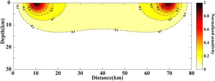
FIGURE 10. Normalized depth sensitivity of scattering waves.

Considering that the static stress rapidly decays as the distance from the epicenter increases, if two stations of a station pair are in different stress-loading regions, the static stress of the station closer to the epicenter exerts a greater impact on the velocity change. For example, the velocity changes for the EYA–TUS, EYA–YUL, BAS–EYA, and HEQ–YUL station pairs were attributed mainly to static stress of the stations closer to the epicenter. According to the meteorological observation data of the Dali Center of the China Earthquake Science Experiment Field, there is no obvious change in the rainfall before and after the main shock (Su et al., 2022). These results suggest that velocity changes are likely linked to a combination of near-surface physical damage and static stress changes. This also explains the inconspicuous drop in the coseismic velocity that was obtained using the autocorrelation for the TUS station, which is closest to the epicenter, compared to those of other nearby stations.

5 Conclusion

In the present study, temporal and spatial coseismic velocity changes were determined for the Yangbi Earthquake using the ambient noise cross-correlation and autocorrelation techniques. The mechanism involved in these velocity changes and effects of clock errors on the measurements were examined. The main conclusions are summarized as follows:

(1) Excluding the LUS station, which is farthest from the epicenter, velocity changes obtained using the single-station autocorrelation indicated declines in the period band of 1–3 s. In contrast, the noise cross-correlation produced both positive and negative velocity changes for 1–10-s period band, and the impact of the Yangbi Earthquake on these velocities lasted for approximately 3 months.

(2) Based on the depth sensitivity of scattering waves, velocity changes that were obtained using the noise cross-correlation produced the largest weight coefficients around the related stations. The static stress of the station closer to the epicenter exerted a greater impact on the velocity change. These observations demonstrated that velocity changes due to a combination of the near-surface physical damage and static stress changes.

(3) Clock errors were obtained in the EYA station, and the time shift for most of 2019 was ∼−.3 s, whereas that for the LUS station between July and August 2021 was ∼−1 s. These time shifts were validated using traveltimes of two groups of nearby teleseismic earthquakes. Clock errors of a few seconds minimally affected velocity measurements using the MWCS method, which estimated a change through linear regression.

Data availability statement

The original contributions presented in the study are included in the article/Supplementary Material, further inquiries can be directed to the corresponding author.

Author contributions

CZ and LF designed this study, analyzed the results, and drafted the manuscript. KS collected the earthquake catalogue and processed the data acquired. XZ and PZ contributed to the discussion and drafting.

Funding

This study is supported by the National Natural Science Foundation of China (Grant No. 41904063, 41974044) and Natural Science Basic Research Program of Shaanxi (Grant No. 2022JQ-256).

Acknowledgments

The authors would like to thank Professor Huajian Yao for using their software to calculate the cross-correlation and autocorrelation functions (http://yaolab.ustc.edu.cn/publication.php). The authors acknowledge that the Data Management Centre of China National Seismic Network at Institute of Geophysics provided the waveform data.

Conflict of interest

The authors declare that the research was conducted in the absence of any commercial or financial relationships that could be construed as a potential conflict of interest.

Publisher’s note

All claims expressed in this article are solely those of the authors and do not necessarily represent those of their affiliated organizations, or those of the publisher, the editors and the reviewers. Any product that may be evaluated in this article, or claim that may be made by its manufacturer, is not guaranteed or endorsed by the publisher.

Supplementary material

The Supplementary Material for this article can be found online at: https://www.frontiersin.org/articles/10.3389/feart.2022.1072017/full#supplementary-material

References

Boschelli, J., Moschetti, M. P., and Sens-Schönfelder, C. (2021). Temporal seismic velocity variations: Recovery following from the 2019 Mw 7.1 ridgecrest, California earthquake. J. Geophys. Res. Solid Earth 126, e2020JB021465. doi:10.1029/2020JB021465

CrossRef Full Text | Google Scholar

Brenguier, F., Campillo, M., Hadziioannou, C., Shapiro, N. M., Nadeau, R. M., and Larose, E. (2008a). Postseismic relaxation along the San Andreas fault at Parkfield from continuous seismological observations. Science 321, 1478–1481. doi:10.1126/science.1160943

PubMed Abstract | CrossRef Full Text | Google Scholar

Brenguier, F., Shapiro, N. M., Campillo, M., Ferrazzini, V., Duputel, Z., Coutant, O., et al. (2008b). Towards forecasting volcanic eruptions using seismic noise. Nat. Geosci. 1, 126–130. doi:10.1038/ngeo104

CrossRef Full Text | Google Scholar

Chaput, J., Campillo, M., Aster, R. C., Roux, P., Kyle, P. R., Knox, H., et al. (2015). Multiple scattering from icequakes at Erebus volcano, Antarctica: Implications for imaging at glaciated volcanoes. J. Geophys. Res. Solid Earth 120, 1129–1141. doi:10.1002/2014JB011278

CrossRef Full Text | Google Scholar

Chen, J., Hao, J., Wang, Z., and Xu, T. (2022). The 21 may 2021 Mw 6.1 Yangbi earthquake—A unilateral rupture event with conjugately distributed aftershocks. Seismol. Res. Lett. 93, 1382–1399. doi:10.1785/0220210241

CrossRef Full Text | Google Scholar

Clarke, D., Zaccarelli, L., Shapiro, N. M., and Brenguier, F. (2011). Assessment of resolution and accuracy of the Moving Window Cross Spectral technique for monitoring crustal temporal variations using ambient seismic noise. Geophys. J. Int. 186, 867–882. doi:10.1111/j.1365-246X.2011.05074.x

CrossRef Full Text | Google Scholar

Clements, T., and Denolle, M. A. (2018). Tracking groundwater levels using the ambient seismic field. Geophys. Res. Lett. 45, 6459–6465. doi:10.1029/2018GL077706

CrossRef Full Text | Google Scholar

Huang, H., Dai, S., and Xie, F. (2021). Monitoring in-situ seismic response on rock slopes using ambient noise interferometry: Application to the 2019 changning (mw 5.7) earthquake, China. Front. Earth Sci. 8. 610181, doi:10.3389/feart.2020.610181

CrossRef Full Text | Google Scholar

Huang, X., Wu, Z., Li, J., Nima, C., Liu, Y., Huang, X., et al. (2014). Tectonic geomorphology and Quaternary tectonic activity in the northwest Yunnan rift zone. Geol. Bull. China 33, 578–593. (in Chinese with English abstract).

Google Scholar

Kanamori, H. (1994). Mechanics of earthquakes. Annu. Rev. Earth Planet. Sci. 22, 207–237. doi:10.1146/annurev.ea.22.050194.001231

CrossRef Full Text | Google Scholar

Le Breton, M., Bontemps, N., Guillemot, A., Baillet, L., and Larose, É. (2021). Landslide monitoring using seismic ambient noise correlation: Challenges and applications. Earth-Science Rev. 216, 103518. doi:10.1016/j.earscirev.2021.103518

CrossRef Full Text | Google Scholar

Li, C., Zhang, J., Wang, W., Sun, K., and Shan, X. (2021). The seismogenic fault of the 2021 Yunnan Yangbi Ms6.4 earthquake. Seismol. Geol. 43, 706–721. (in Chinese with English abstract). doi:10.3969/j.issn.0253-4967.2021.03.015

CrossRef Full Text | Google Scholar

Lin, J., and Stein, R. S. (2004). Stress triggering in thrust and subduction earthquakes and stress interaction between the southern San Andreas and nearby thrust and strike-slip faults. J. Geophys. Res. Solid Earth 109. 2003JB002607, doi:10.1029/2003JB002607

CrossRef Full Text | Google Scholar

Liu, Z., Huang, J., He, P., and Qi, J. (2018). Ambient noise monitoring of seismic velocity around the Longmenshan fault zone from 10 years of continuous observation. J. Geophys. Res. Solid Earth 123, 8979–8994. doi:10.1029/2018JB015986

CrossRef Full Text | Google Scholar

Liu, Z., Huang, J., and Li, J. (2010). Comparison of four techniques for estimating temporal change of seismic velocity with passive image interferometry. Earthq. Sci. 23, 511–518. doi:10.1007/s11589-010-0749-z

CrossRef Full Text | Google Scholar

Liu, Z., Huang, J., Peng, Z., and Su, J. (2014). Seismic velocity changes in the epicentral region of the 2008 Wenchuan earthquake measured from three-component ambient noise correlation techniques. Geophys. Res. Lett. 41, 37–42. doi:10.1002/2013GL058682

CrossRef Full Text | Google Scholar

Liu, Z., Liang, C., Huang, H., Wang, C., and Cao, F. (2022). Seismic velocity variations at different depths reveal the dynamic evolution associated with the 2018 Kilauea eruption. Geophys. Res. Lett. 49, e2021GL093691. doi:10.1029/2021GL093691

CrossRef Full Text | Google Scholar

Mao, S., Campillo, M., van der Hilst, R. D., Brenguier, F., Stehly, L., and Hillers, G. (2019). High temporal resolution monitoring of small variations in crustal strain by dense seismic arrays. Geophys. Res. Lett. 46, 128–137. doi:10.1029/2018GL079944

CrossRef Full Text | Google Scholar

Mao, S., Lecointre, A., van der Hilst, R. D., and Campillo, M. (2022). Space-time monitoring of groundwater fluctuations with passive seismic interferometry. Nat. Commun. 13, 4643. doi:10.1038/s41467-022-32194-3

PubMed Abstract | CrossRef Full Text | Google Scholar

Mao, S., Mordret, A., Campillo, M., Fang, H., and van der Hilst, R. D. (2020). On the measurement of seismic traveltime changes in the time–frequency domain with wavelet cross-spectrum analysis. Geophys. J. Int. 221, 550–568. doi:10.1093/gji/ggz495

CrossRef Full Text | Google Scholar

Meier, U., Shapiro, N. M., and Brenguier, F. (2010). Detecting seasonal variations in seismic velocities within Los Angeles basin from correlations of ambient seismic noise. Geophys. J. Int. 181, 985–996. doi:10.1111/j.1365-246X.2010.04550.x

CrossRef Full Text | Google Scholar

Obermann, A., Planès, T., Hadziioannou, C., and Campillo, M. (2016). Lapse-time-dependent coda-wave depth sensitivity to local velocity perturbations in 3-D heterogeneous elastic media. Geophys. J. Int. 207, 59–66. doi:10.1093/gji/ggw264

CrossRef Full Text | Google Scholar

Obermann, A., Planès, T., Larose, E., Sens-Schönfelder, C., and Campillo, M. (2013). Depth sensitivity of seismic coda waves to velocity perturbations in an elastic heterogeneous medium. Geophys. J. Int. 194, 372–382. doi:10.1093/gji/ggt043

CrossRef Full Text | Google Scholar

Pacheco, C., and Snieder, R. (2005). Time-lapse travel time change of multiply scattered acoustic waves. J. Acoust. Soc. Am. 118, 1300–1310. doi:10.1121/1.2000827

CrossRef Full Text | Google Scholar

Peng, Z., and Ben-Zion, Y. (2006). Temporal changes of shallow seismic velocity around the Karadere-Düzce branch of the north Anatolian fault and strong ground motion. Pure Appl. Geophys. 163, 567–600. doi:10.1007/s00024-005-0034-6

CrossRef Full Text | Google Scholar

Poupinet, G., Ellsworth, W. L., and Frechet, J. (1984). Monitoring velocity variations in the crust using earthquake doublets: An application to the calaveras fault, California. J. Geophys. Res. Solid Earth 89, 5719–5731. doi:10.1029/jb089ib07p05719

CrossRef Full Text | Google Scholar

Reasenberg, P., and Aki, K. (1974). A precise, continuous measurement of seismic velocity for monitoring in situ stress. J. Geophys. Res. Solid Earth 79, 399–406. doi:10.1029/jb079i002p00399

CrossRef Full Text | Google Scholar

Rubinstein, J. L., and Beroza, G. C. (2004). Evidence for widespread nonlinear strong ground motion in the MW 6.9 Loma Prieta earthquake. Bull. Seismol. Soc. Am. 94, 1595–1608. doi:10.1785/012004009

CrossRef Full Text | Google Scholar

Sens-Schönfelder, C., and Wegler, U. (2006). Passive image interferometry and seasonal variations of seismic velocities at Merapi Volcano, Indonesia. Geophys. Res. Lett. 33, L21302. doi:10.1029/2006GL027797

CrossRef Full Text | Google Scholar

Sheng, Y., Ellsworth, W. L., Lellouch, A., and Beroza, G. C. (2021). Depth constraints on coseismic velocity changes from frequency-dependent measurements of repeating earthquake waveforms. J. Geophys. Res. Solid Earth 126, e2020JB020421. doi:10.1029/2020JB020421

CrossRef Full Text | Google Scholar

Snieder, R., Grêt, A., Douma, H., and Scales, J. (2002). Coda wave interferometry for estimating nonlinear behavior in seismic velocity. Science 295, 2253–2255. doi:10.1126/science.1070015

PubMed Abstract | CrossRef Full Text | Google Scholar

Stehly, L., Campillo, M., and Shapiro, N. M. (2007). Traveltime measurements from noise correlation: Stability and detection of instrumental time-shifts. Geophys. J. Int. 171, 223–230. doi:10.1111/j.1365-246X.2007.03492.x

CrossRef Full Text | Google Scholar

Su, J., Yang, W., Li, X., Wang, W., Yang, J., and Chen, Y. (2022). Co-seismic velocity changes with Yunnan Yangbi Ms6.4 earthquake measured by airgun source. Chin. J. Geophys. 65, 649–662. (in Chinese with English abstract). doi:10.6038/cjg2022P0636

CrossRef Full Text | Google Scholar

Vidale, J. E., and Li, Y.-G. (2003). Damage to the shallow Landers fault from the nearby Hector Mine earthquake. Nature 421, 524–526. doi:10.1038/nature01354

PubMed Abstract | CrossRef Full Text | Google Scholar

Wang, B., Zhu, P., Chen, Y., Niu, F., and Wang, B. (2008). Continuous subsurface velocity measurement with coda wave interferometry. J. Geophys. Res. Solid Earth 113, B12313. doi:10.1029/2007JB005023

CrossRef Full Text | Google Scholar

Wegler, U., Nakahara, H., Sens-Schönfelder, C., Korn, M., and Shiomi, K. (2009). Sudden drop of seismic velocity after the 2004M_w6.6 mid-Niigata earthquake, Japan, observed with Passive Image Interferometry. J. Geophys. Res. Solid Earth 114, B06305. doi:10.1029/2008JB005869

CrossRef Full Text | Google Scholar

Yuan, C., Bryan, J., and Denolle, M. (2021). Numerical comparison of time-frequency- and wavelet-domain methods for coda wave interferometry. Geophys. J. Int. 226, 828–846. doi:10.1093/gji/ggab140

CrossRef Full Text | Google Scholar

Zhan, Z., Tsai, V. C., and Clayton, R. W. (2013). Spurious velocity changes caused by temporal variations in ambient noise frequency content. Geophys. J. Int. 194, 1574–1581. doi:10.1093/gji/ggt170

CrossRef Full Text | Google Scholar

Zhang, B., Li, X., Rong, M., Yu, Y., Wang, Y., and Wang, J. (2021). Analysis of strong ground motion characteristics and earthquake damage for the Yangbi Ms6.4 earthquake, Yunnan. Seismol. Geol. 43, 1127–1139. (in Chinese with English abstract). doi:10.3969/j.issn.0253-4967.2021.05.006

CrossRef Full Text | Google Scholar

Zhou, H., Li, Y., and Chang, Y. (2021). Simulation and analysis of spatial distribution characteristics of strong ground motions by the 2021 Yangbi, Yunnan Province Ms6.4 earthquake. Chin. J. Geophys. 64, 4526–4537. (in Chinese with English abstract). doi:10.6038/cjg2021P0421

CrossRef Full Text | Google Scholar

Zhu, G., Yang, H., Tan, Y. J., Jin, M., Li, X., and Yang, W. (2022). The cascading foreshock sequence of the Ms 6.4 Yangbi earthquake in Yunnan, China. Earth Planet. Sci. Lett. 591, 117594. doi:10.1016/j.epsl.2022.117594

CrossRef Full Text | Google Scholar