 Dongil Jang1
 Jae-Kwang Ahn
 Dong Youp Kwak
- 1Department of Civil and Environmental Engineering, Hanyang University, Ansan, South Korea
- 2Earthquake and Volcano Research Division, Korea Meteorological Administration, Seoul, South Korea
This study suggests a linearly combined ground motion model (GMM) optimized for the within-rock conditions of South Korea. Ground motions recorded by accelerometers positioned in within-rock layers are used as target intensity measures (IMs), and five local GMMs and four global GMMs are used as candidates for combination. Optimization, which seeks to find a weight vector minimizing the uncertainty of the combined model, is performed using the quadratic programming (QP) technique, which provides very fast and solid results for the linear combination problem. This study illustrates how to use the QP technique for the linear combination problems. Also, we suggest optimized weight vectors for GMM combinations for two conditions: 1) the IM prediction of a scenario event without observations and 2) the IM prediction of a past event with observations. Among the local and global GMMs considered, JB03, Eea15, JH21, and BSSA14 are selected as the best four GMMs for the first condition, and Jea02, JB03, JH21, and CB14 are selected as the best four GMMs for the second condition. The combined model reduces the standard deviation of residuals in natural logarithms by 10% and 8% for the first and second conditions, respectively, compared to the best individual GMM at each period. Among the GMMs considered, the prediction by Eea15 is only applicable for magnitudes less than 5. Hence, for large magnitude (Mw > 5) prediction, CB14 is recommended instead of Eea15 for the best four models for the first condition.
1 Introduction
After two damaging earthquakes, 2016 ML 5.8 earthquake in Gyeongju and 2017 ML 5.4 earthquake in Pohang, there is a strong need to decide which ground motion model (GMM) or what combination of GMMs is best for the engineering problems (e.g., earthquake early warning and the post-earthquake intensity distribution map). For the development of region-specific GMMs in South Korea, a stochastic method simulating ground motions for the moment magnitude (MW) range of 4–7 and regressing a GMM using simulated intensity measures (IMs) was popular (Noh and Lee, 1995; Jo and Baag, 2001; Jo and Baag, 2003; Park et al., 2001; Junn et al., 2002). There are only limited ground motion records with less than mid-size events (MW ≤ 5.4) in South Korea, so the development of the simulation-based GMM was a reasonable approach to consider the large MW range. Cumulating ground motion records over time with an increased number of seismic stations, some GMMs have been developed empirically (Emolo et al., 2015), but still, the largest MW is low to be considered for the seismic design practice. A hybrid approach, combining empirical data set and ground motion from stochastic simulation, was another way for the GMM development (Jee and Han, 2021).
In the probabilistic seismic hazard assessment, multiple GMMs are combined using a logic-tree approach that assigns appropriate weights to each GMM and linearly combines them (Kramer, 1996). The linear combination of multiple prediction models with appropriate weights reduces the uncertainty of model estimation (Kwak et al., 2018). These weights could be defined based on the rank of GMMs using several ranking procedures (Scherbaum et al., 2009; Kale and Akkar, 2013; Akkar and Kale, 2014; Nizamani and Park, 2021). The ranking provides the order of preference, but it does not suggest the most efficient weights for minimizing the standard deviation of predictions of the combined model. For example, Scherbaum et al. (2009) suggest weights based on the amount of the log-likelihood, but this does not necessarily provide the minimum standard deviation of predictions.
This study suggests the best combination of GMMs with optimized weights minimizing the standard deviation of predictions using the quadratic programming (QP) optimization technique for the IM of ground motion in South Korea. The optimized weights for multiple models were previously found using the Monte Carlo (MC) simulation (Kwak et al., 2018), but the MC simulation is not efficient in terms of execution time and repeatability of the results. QP solves an optimization problem involving a quadratic function (Goldfarb and Idnani, 1983). The QP technique is adopted in this study to find the optimized weights by adjusting the inequality constraints to satisfy the weight conditions of linear combination. The QP is much faster than the MC simulation and provides a solid result.
For the linear combination, five local (JB01, Jo and Baag, 2001; Jea02, Junn et al., 2002; Yea08, Yun et al., 2008; Eea15, Emolo et al., 2015; and JH21, Jee and Han, 2021) and four global (ASK14, Abrahamson et al., 2014; BSSA14, Boore et al., 2014; CB14, Campbell and Bozorgnia, 2014; and CY14, Chiou and Youngs, 2014) GMMs are considered as candidates. The local GMMs were used for the seismic hazard map development (Hong, 2017) and to predict spectral acceleration up to 5 s. To consider IMs for large MW events for the combined GMM, which are out of range for ground motion records in Korea, we also considered four global GMMs from the NGA West2 project (Bozorgnia et al., 2014). We tested the performance of the combined model by comparing it to the seismic records observed during 2000–2018 by the National Seismic Network operated by the Korea Meteorological Administration (KMA).
This study suggests two optimized weight sets: one for a scenario event (where it is anticipated that no records are available) and the other for past events (where it is anticipated that records are available). It should be noted that both weight sets are estimated using ground motion records observed in South Korea. For the scenario event, weights are found based on the total residuals of GMMs. If records are available, the between-event residuals can be calculated, which makes it possible to compute the within-event residuals. Therefore, for the past event, the optimized weight set is suggested, minimizing standard deviation of within-event residuals.
The subsequent sections describe the procedure for solving the weight optimization problem for linear combination, introduce the ground motion data set from South Korea and GMMs, and evaluate the performance of the combined model. Suggestion and conclusion are followed.
2 Quadratic programming defining optimized weights
This section illustrates the linear combination and how to adjust inequality constraints in the QP technique to determine optimized weights in the linear combination problem. This method becomes the base of GMM combinations and provides optimized weight vectors.
The weighted combination of n number of models is expressed as:
where
If we express the residual of the ith model as εi, then the residual of the
This indicates that εcomb is the weighted mean of εi. Then, the variance of εcomb (
where
where w is the wi vector and σ2 is the covariance matrix. w minimizing
Equation 5 is a quadratic function. Hence, finding the object variable (i.e., w) by minimizing the value of Eq. 5 (i.e.,
where x and a are n vectors, G is an n×n symmetric positive definite matrix, C is an n×m matrix, and b is an m vector. Equation 7 contains the quadratic part (
1) Because Eq. 6 does not have a linear part,
2) x and 0.5 G were replaced as w and σ2, respectively;
3) The CT matrix is set as follows (using three models, n = 3 as an example):
4) The b vector is set as follows (using three models, n = 3 as an example):
It should be noted that m becomes n+1 in Eqs 8, 9. For general n, the first row must be set as 1 and an n×n identify matrix from the second for CT, and the first row as 1 and 0 for the last for b. By adjusting CT and b as mentioned previously, Eq. 7 becomes (n = 3 as an example):
The inequality constraint of Eq. 10 indicates:
Since
The QP algorithm is available in several programming languages (e.g., MATLAB, Python, or R). We used the function solve.QP in the quadprog library in R to find the optimized weights (R Core Team, 2022). QP provides the unique w resulting in the smaller
3 Ground motion records and models
3.1 Ground motion records
At the current time (September 2022), KMA maintains 261 seismic observatory stations, and there are 169 outdated stations that were replaced with new sensors or moved to other locations (Korea Meteorological Administration, 2022). Figure 1 shows the locations of all 430 KMA stations. For the stations, there are three stratigraphic levels of sensor locations: 1) surface (0 m depth; called first level hereafter); 2) depth at the top of the bedrock layer, which is defined as the soft rock layer or stiffer (20–70 m depth; called second level hereafter); and 3) 100 m depth (called third level hereafter). The KMA had installed sensors at the first level, but they have been switching the sensor locations to the second or third levels for the purpose of broadband detection of microseisms with minimized ambient noise. For the second-level location, the installation depth is intentionally kept at 20 m even though the bedrock depth is shallower than 20 m. Currently, there are 203 stations that only have sensors at downhole (second and/or third levels), 50 stations that have surface sensors only (first level), and eight stations that have both surface and downhole sensors.
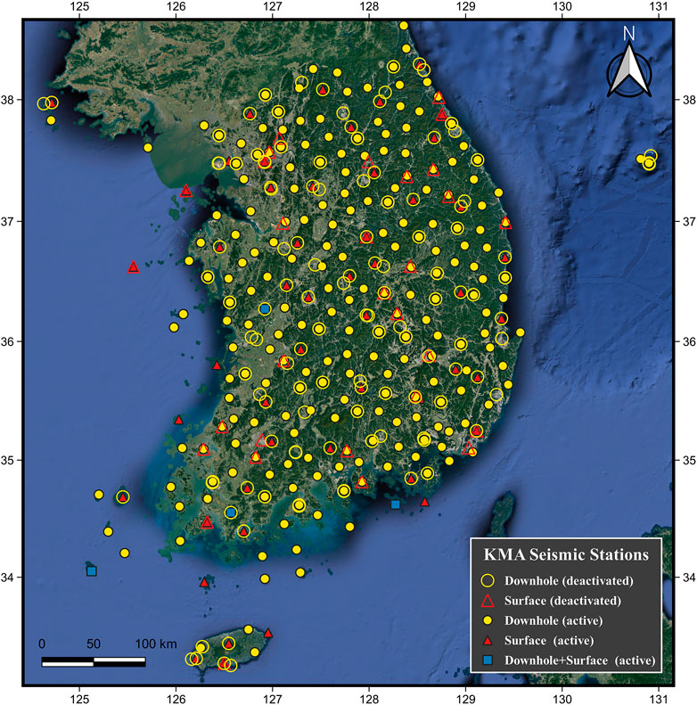
FIGURE 1. Location of KMA seismic stations. Symbol shapes indicate the installation depth of sensors per station, and hollowness distinguishes the operation status.
Among three levels of sensor locations, our interest is in the second level. For practical purposes, predicting IMs at the surface (i.e., first level) is necessary; the seismic hazard analysis of superstructures or geotechnical failure events that occurred at the Earth’s surface (i.e., landslide, lateral spreading, liquefaction, and/or ground settlement) are related to the intensity of the ground motion at the surface. However, the major portion of the KMA sensors is at the second or third levels without sensors at the first level. Moreover, the KMA keeps switching the first level sensors to the second or third levels. This leads to a lack of first-level recordings, which limits the development of a GMM for the surface. To predict first-level IMs, alternatively, an amplification model from the second level to the first level can be coupled with the second-level IM prediction. The third level would have less variability of ground characteristics than the second level, so the GMM targeting the third level would result in less ground motion prediction uncertainty, but the number of records and stations for the third level are less than the second level, and availability of geophysical investigations down to 100 m depth is limited at this time. It should be noted that the data available for the second level are 3,001 records for 207 stations, and the data for the third level are 1,979 records for 65 stations. Hence, in this study, we targeted the second level and used records from the second-level sensors for the target data of the combined GMM.
For the local magnitude (ML) range of 3.5–5.8, the epicentral distance (Repi) range of <210 km, and the time interval between 2000 and 2018, 674 ground motion records have been collected at the second-level sensors. It should be noted that the official magnitude type of earthquake announcement in South Korea is ML, which is used by the KMA. Among these records, we selected 614 ground motions by filtering out poorly recorded ground motions containing very high ambient noise or instrumental errors. We set the lower limit of the ML as 3.5 because it is rare for an event with ML < 3.5 to cause damage to structures, and ML 3.5 is the KMA’s low threshold for the earthquake early warning service. The upper limit of the ML is 5.8 because it is the greatest magnitude recorded in South Korea. The ML versus Repi distribution for the selected records is shown in Figure 2. The major portion of the data is located at the long Repi (>100 km) and small ML (<4).
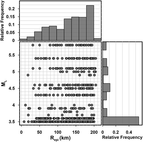
FIGURE 2. Distribution of the local magnitude (ML) and epicentral distance (Repi) of ground motions recorded at the second-level sensors during 2000–2018 by the KMA network.
3.2 Ground motion models
Five region-specific GMMs for South Korea are summarized in Table 1. Three GMMs were developed using stochastic simulation (i.e., random vibration theory; Boore, 1983), one GMM was developed using the empirical data set, and one GMM was developed using the hybrid approach. The stochastic simulation method extracts the stress drop (
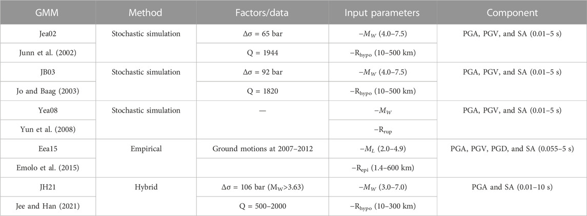
TABLE 1. Comparison of parameters of five Korean-specific GMMs.
The ground motion records collected in this study have limited information: MW or ML, Repi, and hypocentral depth (Zhyp). The ML is available for all ground motions, but MW is only available for large events. To use records with ML as an input parameter for GMM, we transformed ML to MW using the ML–MW relationship suggested for South Korea events (combination of Eq. 8 and Eq. 10 in Sheen et al. (2018)):
It should be noted that the ML in Eq. 13 is the local magnitude suggested by the KMA, and the KMA uses the vertical component for the ML estimation.
Figure 3 compares the selected IMs with respect to varying MW (3–7) at Rhypo = 10, 50, and 200 km. For Eea15, the maximum applicable ML (=4.9) is less than other GMMs, so predictions at large MW are excessively high. Except Eea15, all GMMs have similar magnitude scaling with the non-linear functional shape.
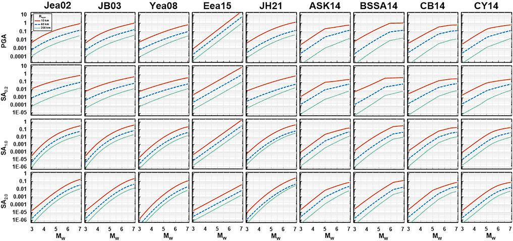
FIGURE 3. Comparison of five Korean GMMs (Jea02, JB03, Yea08, Eea15, and JH21) and four global GMMs (ASK14, BSSA14, CB14, and CY14) for PGA, SA0.2, SA1.0, and SA2.0 with varying MW at Rhypo=10, 50, and 200 km.
Four global GMMs from the NGA West2 project (ASK14, BSSA14, CB14, and CY14) are also considered as candidates for the model combination. NGA West2 GMMs require more detailed input parameters for source, path, and site effects (e.g., fault type, hanging wall effect, depth to the top of the fault, and region) than local GMMs. Table 2 shows the list of input parameters in the NGA West2 project GMMs. However, the data set collected for South Korea only has the parameters MW, Repi, and Zhyp. Hence, we need to assume some parameters for the NGA West2 GMMs with default values. We set up input parameters as “unknown” if applicable, otherwise assigning general values. The fault dip angle, rake angle, and depth to the seismogenic crust (Zbot) need default values, for which 90, 0, and 20 km are used, respectively. We assumed no hanging wall effect, site condition with VS30 = 760 m/s, and an unknown basin depth term. The trends of IMs for NGA West2 GMMs are also shown in Figure 3. It should be noted that the global GMMs have distinct moment saturation points comparing to region-specific GMMs.
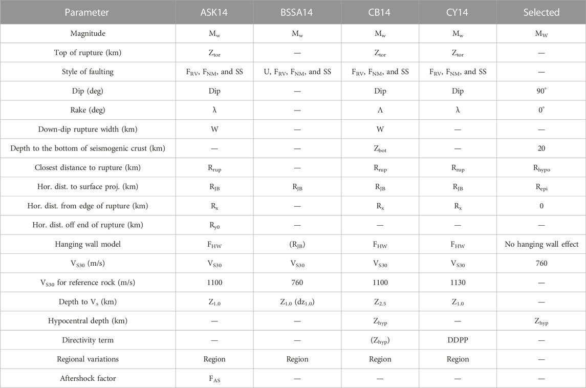
TABLE 2. Variation of input parameters adopted for the model development in the NGA West2 project and parameters selected to use for Korean event prediction.
4 Residual analysis
4.1 Site condition adjustment
The target site conditions of five local GMMs are rock outcrop, and those of global GMMs are surfaces with varying VS30. However, the target site condition in this study is the within-rock layer (i.e., second level), and within-rock layer records are collected. Hence, we expect that direct comparison of GMM predictions with the collected records is not appropriate—predictions (surface) would be larger than observations (within-rock). Figure 4 shows boxplots of total residuals (restt) per GMM. Generally, the medians (centerline of the box) of restt are smaller than zero for local GMMs for a wide range of periods, but those for global GMMs are period-dependent. For long periods (SA1.0), medians are less than zero, but for low periods (PGA and SA0.2), medians are greater than zero. This means that for local GMMs, most ground motion observations are lower than predictions as expected, but the global GMMs predict too low IMs for certain periods. This might be attributed to the fact that the global GMMs were developed using ground motion records from different regions.
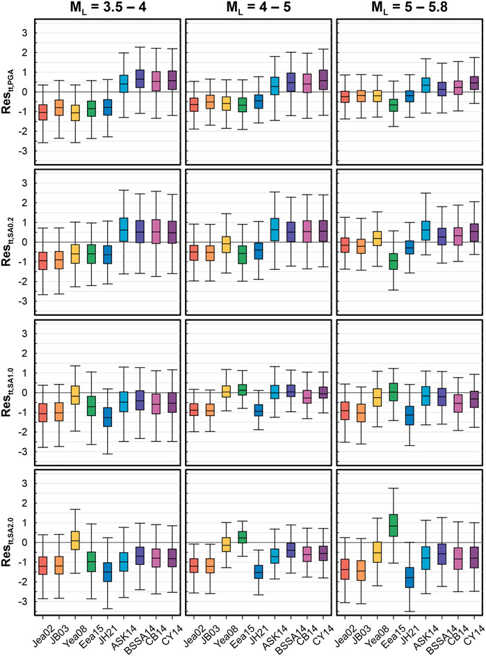
FIGURE 4. Total residual boxplots of four IMs (PGA, SA0.2, SA1.0, and SA2.0) binned by ML for nine GMMs.
To remove this discrepancy arising from the difference of the target site condition and regional difference, we omitted the global bias of restt by performing mixed-effect linear regression. The mixed-effect linear regression provides random effects and fixed effects, where the fixed effects are equivalent to the global bias of restt, the random effects are between-event residuals, and the remaining are the within-event residuals (Abrahamson and Youngs, 1992; Boore et al., 2014). Using the mixed-effect linear regression, restt can be disintegrated as:
where ck is the global bias for model k,
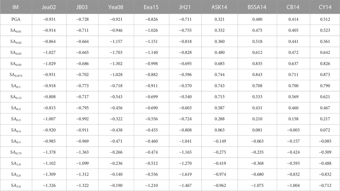
TABLE 3. Global bias of the mixed-effect linear regression for five local and four global GMMs.
4.2 Comparison of GMM performance
Figure 5 shows the standard deviation of restt (denoted σtt),
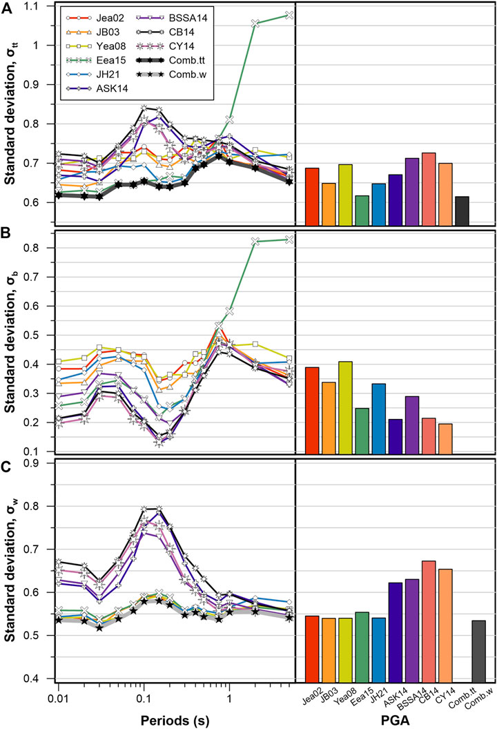
FIGURE 5. Standard deviation of (A) total residuals, (B) between-event residuals, and (C) within-event residuals for nine individual GMMs and combined GMMs suggested in this study.
5 Performance of combined GMM
5.1 Selection of best combination
For the sake of the IM prediction for future earthquakes, we cannot specify
In practice, for simplicity, using two to four GMMs is preferable for the combination rather than use of several to tens of GMMs. Hence, in this section, we examine the efficiency of the model combination using different numbers of GMMs. Among the nine GMMs (five local and four global), we picked one to five GMMs as combination candidates and found the optimized weights using the QP process. The QP process is summarized as follows:
1) The covariance matrix (σ2 in Eq. 6 and Eq. 10) of the restt and δWes between GMMs selected was calculated;
2) σ2 is inserted into Eq. 10;
3) The optimized w is calculated.
It should be noted that the QP should have σ2 as the positive definite matrix, so we slightly altered σ2 to be the nearest positive definite matrix using the nearPD function in R (Higham, 2002) if σ2 is not positively definite. Figure 6 shows the average of σtt and σw of IMs including PGA and 15 kinds of SAs ranging from 0.01 to 5 s of the best combined models for different number of model combination. The standard deviation is the highest for a single GMM case, and it decreases steeply for the case of a combination of two models. The standard deviations are decreasing with the greater number of GMM combinations, but the reduction rate slows down. Table 4 shows the GMMs selected for the best combination for different numbers of models and indicates the percentage difference in average standard deviation compared to the combination of all nine GMMs. The single best GMM has 10.2% larger σtt than one from a nine-GMM combination and 8.45% larger σw than one from nine GMM combination, but the difference becomes small if the number of GMMs for combination increases. The differences of average standard deviation between a four-GMM combination and a nine-GMM combination become negligible (less than 0.2%), so we selected a four-GMM combination as the suggested GMM model in this study.
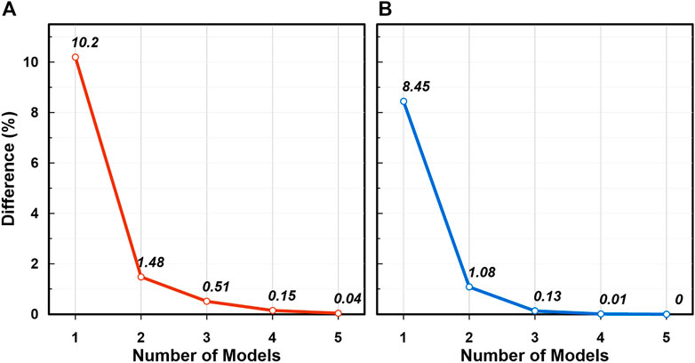
FIGURE 6. Percentage difference of standard deviation between one from the combination of nine GMMs and the other from a combination of different numbers of GMMs. (A) σtt and (B) σb.
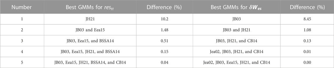
TABLE 4. Best GMMs for different numbers of candidates.
Table 5 describes the optimized weights suggested for restt and
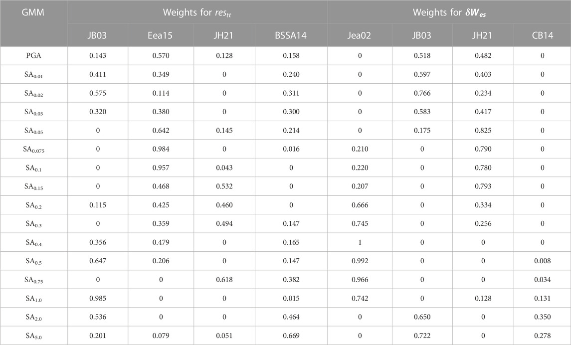
TABLE 5. Suggested weights of four GMMs for restt and
5.2 Performance of combined GMM compared to records
To evaluate the performance of the combined GMM, we compared the median predictions of the GMMs with the recorded distribution. Figure 7 shows observed IMs (PGA, SA0.2, SA1.0, and SA3.0), median IMs of six GMMs (Jea02, JB03, Eea15, JH21, BSSA14, and CB14) adjusted by ck (Table 3), and median IMs of two combined GMMs minimizing σtt and σw using optimized weights (Table 5). For the comparison, we made two groups: 1) observed IMs with ML 3.5–4.5 and median prediction of GMMs using ML = 3.6, that is, the median ML of the observed IMs and 2) observed IMs with ML 4.5–5.8 and median prediction of GMMs using ML = 5.1, that is, the median ML of the observed IMs. Binned means of observed IMs are also shown in Figure 7. The combined GMM minimizing σtt (denoted Combtt) fits well with the observations for all IMs considered. Because
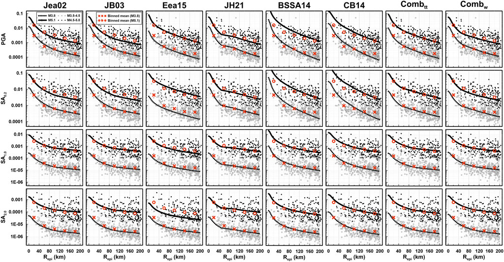
FIGURE 7. Comparison of four modified Korean GMMs and two global GMMs (Jea02, JB03, Eea15, JH21, BSSA14, and CB14) with combined GMMs minimizing σtt and σw (Combtt and Combw, respectively) for PGA, SA0.2, SA1.0, and SA2.0 with ML = 3.6 and 5.1 varying Repi. Records and binned means for ML 3.5–4.5 and ML 4.5–5.8 are overlapped.
5.3 GMMs for large magnitude
The suggested GMMs (Combtt and Combw) mentioned earlier were tested with ground motion records with ML ≤ 5.8. In South Korea, however, the magnitude range of 6.0–7.0 is used for seismic design practice (Earthquake Engineering Society of Korea, 2018), for which local records are not available. To check the effectiveness of the suggested GMM for this extrapolated range of magnitude, this section compares the trend of Combtt and Combw with the NGA West2 GMMs, which were developed using large magnitude ground motion records—the minimum of the upper limit MW is 7.5.
Figure 8 shows selected IMs including PGA, SA0.1, SA0.2, SA0.5, SA1.0, and SA2.0 with an increase of MW from 5 to 7.5. For this calculation, Repi and Rjb are set to 20 km, Zhyp is set to 10 km, and other parameters for NGA West2 GMMs are set as shown in Table 2. The Combtt and Combw are extrapolated up to MW 7.5 and compared with the NGAW2eq (a combined GMM with equal weights for the four NGA West2 models with mean bias correction using coefficients from Table 3). At low periods (PGA and SA ≤ 0.5 s), the IMs of Combtt increase linearly, so they become excessively high at large magnitudes. This is attributed to the fact that Eea15 has higher weights at low periods (Table 5), and the magnitude application range of Eea15 is less than 5. Hence, including Eea15 in the Combtt is not appropriate if Combtt is used for MW > 5. For Combw, on the other hand, the trend of magnitude saturation is comparable with the NGAW2eq. The best four GMMs selected for Combw do not include Eea15 (Table 4), and the MW range is up to 7 (Table 1). It means that Combw could be used for large MW events (>5) even though it is not validated with observed IMs.
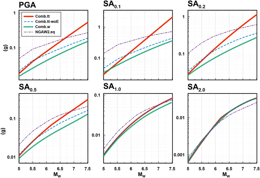
FIGURE 8. Comparison of magnitude scaling of PGA, SA0.1, SA0.2, SA0.5, SA1.0, and SA2.0 for combined GMMs (Combtt, Combtt-woE, and Combw) with equally weighted NGA W2 models (NGAW2.eq).
For the suggestion of Combtt for large MW, we omitted Eea15 and found the best four GMMs and their weights as indicated in Table 6. The trend of magnitude saturation of this model (Combtt-woE) is shown in Figure 8, which is comparable to NGAW2eq for all spectral periods. However, the difference in average standard deviation of the Combtt-woE is 1.62% compared to all nine models (Figure 4), which is higher than the difference of Combtt (0.15%). Hence, it is recommended to use Combtt for small MW, which is the optimized model, and use Combtt-woE for large MW, which avoids excessive extrapolation at large MW.

TABLE 6. Suggested GMMs and weights minimizing σtt per IM for large MW (>5).
6 Conclusion
This study suggests the best combination of GMMs for within-rock layer ground motion in South Korea. Local and global GMMs were used for model combination, and ground motions recorded in the within-rock layer were used for validation. The optimized weights were found using the QP technique, which provides fast and solid results in the model combination problem and effectively selects GMMs for the best combination, which minimizes the uncertainty of the combined model. Two cases of optimized weights were suggested: the first case for the prediction without ground motion observations (e.g., a future or scenario event) and the second case for the prediction with observations (e.g., a past event with ground motion records). Among the five local and four global GMMs considered, a combination of JB03, Eea15, JH21, and BSSA14 is suggested for the first case with small MW (MW < 5), and a combination of JB03, JH21, BSSA14, and CB14 is recommended for large MW (MW ≥ 5). The combination of Jea02, JB03, JH21, and CB14 is evaluated as the best for the second case. The performance was evaluated by comparing the standard deviation of the model residuals. The combined model reduces the average standard deviation of residuals by up to 10% compared to the best single GMM. The combination of even two models reduces the standard deviation significantly. The combined GMMs were also compared with equally weighted global GMMs for larger magnitudes where ground motion records for South Korea are not available. This comparison revealed that the suggested combined GMMs are applicable up to MW = 7.5. The linear combination using the optimized weights suggested in this study minimizes the standard deviation of the residuals of the combined model.
The limitation of this study is that the suggested method is based on the empirical data, so records are required for the estimation of optimized weights and for the removal of the mean misfit. Also, the model uncertainty would be increased for the ground motions, for which the magnitude and distance were not covered in this study. In addition, the suggested model is for the within-rock condition, so coupling with site amplification is required to estimate ground motion amplitudes at the surface. The suggested model provides PGA and spectral accelerations for periods from 0.01 to 5 s given earthquake magnitude and hypocentral distance, but a recent study reveals that the near-fault effect such as a pulse-like seismic wave can result in more serious damage for slopes for the same magnitude and distance (Zhu et al., 2020; Zhu et al., 2022). The future studies will find optimized weights without records, estimate model uncertainty for ground motions, which are out of the range of the dataset, couple with a site amplification model and validate with surface ground motion records, and find the GMMs that consider near-fault effects, as promised.
Data availability statement
The raw data supporting the conclusion of this article will be made available by the authors, without undue reservation.
Author contributions
DK, J-KA, and T-WK contributed to the conception and design of the study. DJ organized and analyzed the database and prepared figures. DJ and DK wrote the first draft of the manuscript. JK-A and T-WK reviewed and analyzed the results and recommended corrections. All authors contributed to manuscript revision, read, and approved the submitted version.
Funding
This work was supported by the Hanyang University (grant number HY-2019-N) and the Korea Meteorological Administration (grant number KMA2022-02121).
Acknowledgments
Authors greatly appreciate Hanyang University and KMA's supports. Any opinions, findings, and conclusions or recommendations expressed in this material are those of the authors and do not necessarily reflect those of the Hanyang University and KMA.
Conflict of interest
The authors declare that the research was conducted in the absence of any commercial or financial relationships that could be construed as a potential conflict of interest.
Publisher’s note
All claims expressed in this article are solely those of the authors and do not necessarily represent those of their affiliated organizations, or those of the publisher, the editors, and the reviewers. Any product that may be evaluated in this article, or claim that may be made by its manufacturer, is not guaranteed or endorsed by the publisher.
References
Abrahamson, N. A., Silva, W. J., and Kamai, R. (2014). Summary of the ASK14 ground motion relation for active crustal regions. Earthq. Spectra 30, 1025–1055. doi:10.1193/070913eqs198m
Abrahamson, N. A., and Youngs, R. R. (1992). A stable algorithm for regression analyses using the random effects model. Bull. Seismol. Soc. Am. 82, 505–510. doi:10.1785/bssa0820010505
Akkar, S., and Kale, Ö. (2014). Reply to “comment on ‘A new procedure for selecting and ranking ground-motion prediction equations (GMPEs): The Euclidean distance-based ranking (EDR) method’ by Özkan Kale and Sinan Akkar” by Sum Mak, Robert Alan Clements, and Danijel Schorlemmer. Bull. Seismol. Soc. Am. 104, 3141–3144. doi:10.1785/0120140169
Al Atik, L., Abrahamson, N., Bommer, J. J., Scherbaum, F., Cotton, F., and Kuehn, N. (2010). The variability of ground-motion prediction models and its components. Seismol. Res. Lett. 81, 794–801. doi:10.1785/gssrl.81.5.794
Boore, D. M., Stewart, J. P., Seyhan, E., and Atkinson, G. M. (2014). NGA-West2 equations for predicting PGA, PGV, and 5% damped PSA for shallow crustal earthquakes. Earthq. Spectra 30, 1057–1085. doi:10.1193/070113eqs184m
Boore, D. M. (1983). Stochastic simulation of high-frequency ground motions based on seismological models of the radiated spectra. Bull. Seismol. Soc. Am. 73, 1865–1894. doi:10.1785/BSSA07306A1865
Bozorgnia, Y., Abrahamson, N. A., Al Atik, L., Ancheta, T. D., Atkinson, G. M., Baker, J. W., et al. (2014). NGA-West2 research project. Earthq. Spectra 30, 973–987. doi:10.1193/072113eqs209m
Campbell, K. W., and Bozorgnia, Y. (2014). NGA-West2 ground motion model for the average horizontal components of PGA, PGV, and 5% damped linear acceleration response spectra. Earthq. Spectra 30, 1087–1115. doi:10.1193/062913eqs175m
Chiou, B. S.-J., and Youngs, R. R. (2014). Update of the Chiou and Youngs NGA model for the average horizontal component of peak ground motion and response spectra. Earthq. Spectra 30, 1117–1153. doi:10.1193/072813eqs219m
Earthquake Engineering Society of Korea (EESK) (2018). Commentary of general seismic design code. KDS 17 (10 00), 2018.
Emolo, A., Sharma, N., Festa, G., Zollo, A., Convertito, V., Park, J. H., et al. (2015). Ground-motion prediction equations for South Korea Peninsula. Bull. Seismol. Soc. Am. 105, 2625–2640. doi:10.1785/0120140296
Goldfarb, D., and Idnani, A. (1983). A numerically stable dual method for solving strictly convex quadratic programs. Math. Program. 27, 1–33. doi:10.1007/bf02591962
Higham, N. (2002). Computing the nearest correlation matrix - a problem from finance. IMA J. Numer. Anal. 22, 329–343. doi:10.1093/imanum/22.3.329
Hong, T. K. (2017). Establishment of standardized procedure and development of national seismic hazard maps Report R&D 2017-MPSS31-107. Sejong, Korea: Ministry of Interior and Safety, 635. (in Korean).
Jee, H. W., and Han, S. W. (2021). Regional ground motion prediction equation developed for the Korean Peninsula using recorded and simulated ground motions. J. Earthq. Eng. 26, 5384–5406. doi:10.1080/13632469.2021.1871682
Jo, N., and Baag, C. (2003). Estimation of spectrum decay parameter k and stochastic prediction of strong ground motions in southeastern Korea. J. Earthq. Eng. Soc. Korea 7, 59–70. (in Korean). doi:10.5000/EESK.2003.7.6.059
Jo, N., and Baag, C. (2001). Stochastic prediction of strong ground motions in southern Korea. J. Earthq. Eng. Soc. Korea 5, 17–26. (in Korean).
Junn, J.-G., Jo, N.-D., and Baag, C.-E. (2002). Stochastic prediction of ground motions in southern Korea. Geosci. J. 6, 203–214. doi:10.1007/bf02912691
Kale, Ö., and Akkar, S. (2013). A new procedure for selecting and ranking ground-motion prediction equations (GMPEs): the Euclidean distance-based ranking (EDR) method. Bull. Seismol. Soc. Am. 103, 1069–1084. doi:10.1785/0120120134
Korea Meteorological Administration (KMA) (2022). National earthquake comprehensive information system (NECIS). Available at: https://necis.kma.go.kr/ (Accessed September 22, 2022).
Kwak, D. Y., Seyhan, E., and Kishida, T. (2018). “A method of linear combination of multiple models for epistemic uncertainty minimization,” in 11th National Conference on Earthquake Engineering, Los Angeles, CA, 25–29 June, 2018.
Nizamani, Z. A., and Park, D. (2021). Testing ground-motion prediction equations against moderate magnitude earthquake data recorded in Korea. Bull. Seismol. Soc. Am. 111, 321–338. doi:10.1785/0120200095
Noh, M. H., and Lee, K. H. (1995). Estimation of peak ground motions in the Southeastern part of the Korean peninsula (II): Development of predictive equations. J. Geol. Soc. Korea 31, 175–187. (in Korean).
Park, D. H., Lee, J. M., Baag, C.-E., and Kim, J. K. (2001). Stochastic prediction of strong ground motions and attenuation equations in the southeastern Korean Peninsula. J. Geol. Soc. Korea 37, 21–30. (in Korean).
R Core Team (2022). R: A language and environment for statistical computing. Vienna, Austria: R Foundation for Statistical Computing.
Scherbaum, F., Delavaud, E., and Riggelsen, C. (2009). Model selection in seismic hazard analysis: An information-theoretic perspective. Bull. Seismol. Soc. Am. 99, 3234–3247. doi:10.1785/0120080347
Sheen, D.-H., Kang, T.-S., and Rhie, J. (2018). A local magnitude scale for South Korea. Bull. Seismol. Soc. Am. 108, 2748–2755. doi:10.1785/0120180112
Yun, K.-H., Park, D.-H., Chang, C.-J., and Sim, T.-M. (2008). “Estimation of aleatory uncertainty of the ground-motion attenuation relation based on the observed data,” in Proceedings of EESK conference, Seoul, Korea, 21 March, 2008, 116–123.
Zhu, C., Cheng, H., Bao, Y., Chen, Z., and Huang, Y. (2022). Shaking table tests on the seismic response of slopes to near-fault ground motion. Geomech. Eng. 29 (2), 133–143.
Keywords: linear combination, optimized weights, quadratic programming, ground motion model, within-rock records, South Korea
Citation: Jang D, Ahn J-K, Kim T-W and Kwak DY (2023) Linearly combined ground motion model using quadratic programming for low- to mid-size seismicity region: South Korea. Front. Earth Sci. 10:1067802. doi: 10.3389/feart.2022.1067802
Received: 12 October 2022; Accepted: 14 December 2022;
Published: 05 January 2023.
Edited by:
Gerardo Grelle, Faculty of Civil and Industrial Engineering, Sapienza University of Rome, ItalyReviewed by:
Min Xiong, Tongji University, ChinaChongqiang Zhu, University of Dundee, United Kingdom
Copyright © 2023 Jang, Ahn, Kim and Kwak. This is an open-access article distributed under the terms of the Creative Commons Attribution License (CC BY). The use, distribution or reproduction in other forums is permitted, provided the original author(s) and the copyright owner(s) are credited and that the original publication in this journal is cited, in accordance with accepted academic practice. No use, distribution or reproduction is permitted which does not comply with these terms.
*Correspondence: Dong Youp Kwak, ZGt3YWtAaGFueWFuZy5hYy5rcg==