Numerical modelling of an alpine debris flow by considering bed entrainment

Numerical models have become a useful tool for predicting the potential risk caused by debris flows. Although a variety of numerical models have been proposed for the runout simulation of debris flows, the performances of these models in simulating specific events generally vary due to the difference in solving methods and the simulation of the entrainment/deposition processes. In this paper, two typical depth-averaged models have been used to analyze a well-documented debris-flow event that occurred in the Cancia basin on 23 July 2015. The simulations with and without bed entrainment are conducted to investigate the influence of this process on the runout behavior of the debris flow. Results show that the actual runout can be reproduced only by considering bed entrainment. If basal erosion is not taken into account, part of the debris mass deviates from the main path and both models predict unrealistic bank overflows not observed in the field. Moreover, the comparison between measured and simulated inundated areas shows that both models perform generally well in the terms of simulating the erosion-deposition pattern, although the DAN3D model predicts a greater lateral spreading and a thinner depositional thickness compared to Shen’s model. A simple numerical experiment obtains similar consequences and further illustrates the possible reasons that cause these differences.

1 Introduction

Debris flows are mass movements consisting of saturated particles of a wide range of sizes, occurring periodically along pre-existing channels in mountainous areas (Hungr et al., 2001). These flows are usually characterized by high velocity, large impact force, and long run-out distance and are considered as one type of the most catastrophic landslides (Hutter et al., 1996; Jakob and Hungr, 2005; Takahashi, 2014). Runoff-generated debris flows commonly occur in the Alpine region and their frequency seems to be increasing due to the effects of climate change, which is leading to increase of both extreme rainfalls (Bollschweiler and Stoffel, 2010) and rock-collapse events providing debris material (Damm and Felderer, 2013; Stoffel et al., 2014; Draebing and Krautblatter, 2019; Rengers et al., 2020).

In the last decades, many different numerical models for the simulation of debris flows and flow-like landslides have been developed. Due to the simpler governing equations and less computational time compared with the fully 3D numerical models, such as the 3D models based on smoothed particle hydrodynamics (SPH) (Wang et al., 2016; Dai et al., 2017), material point method (MPM) (Li et al., 2020; Vicari et al., 2022) and particle finite element method (PFEM) (Zhang et al., 2020; Wang and Zhang, 2022), depth-averaged models derived from the principles of continuum mechanics have been widely applied to reproduce and analyze the dynamic processes of flow-like landslides. The unsteady debris flow model for simulating erosion/deposition process of sediment during the flow was proposed (Chen, 1987). Savage and Hutter (1989) pioneered the work in this field by developing a depth-averaged model for the simulation of granular flow. O’Brien et al. (1993) conceived the 2D finite difference model (FLO-2D) for the modeling of debris and mud flow, based on Saint–Venant equations. Later Armanini et al. (2009) and Frank et al. (2015) introduced finite-volume codes also simulating entrainment in the case of bi-phase and mono-phase continuums respectively. SCIDDICA S_3–hex was developed for simulating debris flow and calibrated by considering several real cases of debris flows that occurred in Campania (Southern Italy) in May 1998 and December 1999 (D’Ambrosio et al., 2003). In 1995, Hungr presented the popular DAN-W model based on the concept of “equivalent fluid”. Since then, several modified models have been proposed and tested with actual field cases: RAMMS-DF, a rapid mass movement simulation model designed to simulate the runout of muddy and debris-laden flows in complex terrain (Christen et al., 2010); Frimberger et al. (2021)back-calculated the well-documented 1877 lahar using the RAMMS-DF model with an implemented entrainment algorithm and developed a generic Voellmy–Salm approach across different scales of high-magnitude lahars to anticipate potential lahars. LS-RAPID, a 3D landslide simulation model, originally developed by Sassa (1988) and further improved by Sassa et al. (2010); DAN3D, developed by McDougall and Hungr (2004) to analyze the rapid mass motion across 3D terrain. More recently, Ouyang et al. (2013) proposed a massflow model in which the depth-averaged equation was solved in the MacCormack-TVD finite difference scheme, and Shen et al. (2018) presented a modified finite difference model for flow-like type able to capture debris flow propagation over complex topographies. With the rapid development of computing technology, depth-averaged models were further developed. Pastor et al. (2015, 2014, 2009) proposed innovative depth-averaged SPH models able to simulate the propagation process of rapid landslide, while Lin et al. (2019) developed a depth-integrated SPH model to reproduce the Lo Wai debris flood. The depth-averaged material point method (DAMPM) was proposed by Abe et al. (2007) and then widely applied to analyze many actual debris-flow events (Kazmi et al., 2012, 2014). More recently, the DAMPM incorporating the excess pore water pressure was developed by Abe and Konagai (2016) to better simulate the runout process of actual debris flows. The depth-averaged numerical models mentioned above are mainly generalized into two categories: mesh-based methods such as finite volume method (FVM) and finite difference method (FDM), and particle-based methods such as SPH and MPM. Due to Eulerian mesh discretization, the mesh-based models cannot track the internal deformation of debris mass during the propagation of debris flow. However, this problem is successfully solved in particle-based models. Although models belonging to both categories have numerous successful applications in predicting inundated areas, runout distances and final depths of deposits (Pastor et al., 2014; Abe and Konagai, 2016; Bao et al., 2019; Zhang et al., 2021) and comparisons of different numerical models for simulating the actual debris flow event have been carried out by many previous researchers in the last decades (Sauthier et al., 2015; Vagnon et al., 2019; Mousavi Tayebi et al., 2021), some issues are still unclear, such as the performance of different numerical models under the erosion condition. Moreover, there are few papers comparing the results of modelling to real erosion/deposition patterns due to the lack of field data (Medina et al., 2008; Han et al., 2015; Guo et al., 2022). However, this goal is available in our study area as Simoni et al. (2020) described the geomorphological variations induced by debris flow along the channel in detail.

A crucial aspect that distinguishes these models is the ability to reproduce bed entrainment. Sediment entrainment is a fundamental process in debris flow dynamics, and it is responsible of the increase of flow volume along the channel commonly observed in the field (Han et al., 2015; Gregoretti et al., 2018). However, including bulking due to entrainment in depth-averaged models is difficult. Several models tried to consider entrainment using empirical laws that assume a proportional relationship between flow velocity (v) and flow depth (h) (McDougall and Hungr, 2005; Pirulli and Pastor, 2012). These empirical models provide a simple way to estimate the volume increasing during the entrainment process but are unable to explain the physical mechanism of the entrainment. Recently, some process-based entrainment models have been developed to address this limitation (Iverson, 2012; Han et al., 2015; Ouyang et al., 2015; Shen et al., 2019, 2022).

The objective of this paper is to evaluate the performance of two models in reproducing a debris flow that recently occurred in the Dolomites of Italy (Northern Alps). Specifically, we aim to simulate the debris flow propagation including erosive and depositional processes occurred along the channel, until its final deposition. The 23 July 2015 debris flow event that occurred in the Cancia basin is chosen as the test case because monitoring data in combination with topographic and UAV (Unmanned Aerial Vehicle) surveys document the debris flow process and the morphological changes along the channel. For volume-enlarging debris flow (Berti et al., 1999; Breien et al., 2008; Berti and Simoni, 2014), the entrainment cannot be ignored to accurately predict the final magnitude of debris flows (Pudasaini and Fischer, 2020). For this reason, two typical depth-averaged models that account for bed entrainment (Shen’s model and DAN3D code) are used to carry out a back analysis of the event. The DAN3D model (McDougall and Hungr, 2004), a commercial code based on smoothed particle hydrodynamics (SPH) method, is widely used for the prediction of the movement and the velocity of a rapid flow slide. Shen’s model (Shen et al., 2018), a modified finite difference program, is suitable for dynamic simulation of fluid-like flow. Model calibration was carried out by comparing observed and computed characteristics of the deposits for a good-fit in terms of flow depth, inundated area, overall volume and shape of their boundaries.

The paper is structured into the following sections. In Sect. 2 the methodologies, i.e., the two numerical methods and the implementation of rheology and entrainment for both models, are briefly introduced. Then in Sect. Three some simple numerical experiments are performed to illustrate the performance of the two models. Following which, the Cancia debris flow channel and the July 23 debris flow event are described in Sect. 4, and the computational model, simulation setup and comparison of simulation results of the debris flow are presented in Sect. 5. Finally, the main conclusions are presented in Sect. 6.

2 Methodologies

2.1 General concepts and governing equation

DAN3D is a SPH-based numerical model developed by McDougall and Hungr (2004) for the dynamic analysis of rapid flow slides, debris flows, and rock avalanches. In this model, the flow is simplified as an incompressible equivalent fluid. This method uses the continuous Lagrangian approach for integrating the governing equations in the depth direction. Furthermore, the depth-integrated equations are deduced in a local Cartesian coordinate system (x, y, z), the axis of z points outward normal to the sliding surface. The governing equations can be expressed as follows:

$\frac{\partial \mathit{h}}{\partial \mathit{t}}+\frac{\partial \left({\mathit{v}}_{\mathit{x}}\mathit{h}\right)}{\partial \mathit{x}}+\frac{\partial \left({\mathit{v}}_{\mathit{y}}\mathit{h}\right)}{\partial \mathit{y}}+\frac{\partial \mathit{b}}{\partial \mathit{t}}=\mathbf{0}(1)$

$\mathit{\rho }\frac{\partial \left({\mathit{v}}_{\mathit{x}}\mathit{h}\right)}{\partial \mathit{t}}=\mathit{\rho }\mathit{h}{\mathit{g}}_{\mathit{x}}+{\mathit{k}}_{\mathit{x}}{\mathit{\sigma }}_{\mathit{z}}\left(-\frac{\partial \mathit{h}}{\partial \mathit{x}}\right)+{\mathit{k}}_{\mathit{y}\mathit{x}}{\mathit{\sigma }}_{\mathit{z}}\left(-\frac{\partial \mathit{h}}{\partial \mathit{y}}\right)+{\mathit{\tau }}_{\mathit{z}\mathit{x}}-\mathit{\rho }{\mathit{v}}_{\mathit{x}}\frac{\partial \mathit{b}}{\partial \mathit{t}}(2)$

$\mathit{\rho }\frac{\partial \left({\mathit{v}}_{\mathit{y}}\mathit{h}\right)}{\partial \mathit{t}}=\mathit{\rho }\mathit{h}{\mathit{g}}_{\mathit{y}}+{\mathit{k}}_{\mathit{y}}{\mathit{\sigma }}_{\mathit{z}}\left(-\frac{\partial \mathit{h}}{\partial \mathit{y}}\right)+{\mathit{k}}_{\mathit{x}\mathit{y}}{\mathit{\sigma }}_{\mathit{z}}\left(-\frac{\partial \mathit{h}}{\partial \mathit{x}}\right)+{\mathit{\tau }}_{\mathit{z}\mathit{y}}-\mathit{\rho }{\mathit{v}}_{\mathit{y}}\frac{\partial \mathit{b}}{\partial \mathit{t}}(3)$

where $\rho$ is the bulk density of the debris mass and the erodible material, $h$ is the bed-normal flow depth, $v_x$ and $v_y$ are the local flow velocities, and $b$ is the bed-normal entrained depth, $\partial b/\partial t$ represents the entrainment rate of material, $g_x$ and $g_y$ are the components of the acceleration of gravity in the x and y directions, respectively, ${\sigma }_z$ is the bed-normal stress, ${\tau }_{zx}$ and ${\tau }_{zy}$ are the basal stress in the x and y directions, respectively, $k_x$, $k_{yx}$, $k_{xy}$ and $k_y$ are the stress coefficients.

The time term on the left side of Eq. 2 and 3 represents the variation of momentum fluxes per unit basal area; the first four terms represent the momentum fluxes due to the gravity, normal stress, transvers shear stress and basal shear stress, respectively. The last term refers to the momentum fluxes due to the entrainment.

In Eqs (2), (3), $k_x$ and $k_y$ vary with time and space. In accord with the classical Rankine theory, the stress coefficients are limited and determined by the state (i.e., active, static, or passive state) of the sliding mass, as suggested by Savage and Hutter (1989). In the DAN3D model, a modified equation was proposed by McDougall and Hungr (2004).

$\left.\begin{array}{c}{\mathit{k}}_{\mathit{x}\left(\mathit{min}\right)}={\mathit{k}}_{\mathit{a}\mathit{c}\mathit{t}}\\ {\mathit{k}}_{\mathit{x}\left(\mathit{max}\right)}={\mathit{k}}_{\mathit{p}\mathit{a}\mathit{s}}\end{array}\right\}=\mathbf{2}\left[\frac{\mathbf{1}\mp \sqrt{\mathbf{1}-{\mathit{cos}}^{\mathbf{2}}{\varnothing }_{\mathit{i}}\left(\mathbf{1}+{\mathit{k}}_{\mathit{z}\mathit{x}}^{\mathbf{2}}\right)}}{{\mathit{cos}}^{\mathbf{2}}{\varnothing }_{\mathit{i}}}\right]-\mathbf{1}(4)$

where $k_{act}$ and $k_{pas}$ are the minimum and maximum limiting values of the stress coefficient. ${\varnothing }_i$ is the internal friction angle, and $k_{zx}$ is determined by ${\tau }_{zx}/{\sigma }_z$, which is less than $\tan {\varnothing }_i$.

The limiting of $k_y$ is given by:

$\left\{\begin{array}{c}{\mathit{k}}_{\mathit{y}\left(\mathit{min}\right)}=\left[\left(\frac{{\mathit{k}}_{\mathit{x}}+\mathbf{1}}{\mathbf{2}}\right)+\sqrt{{\left(\frac{{\mathit{k}}_{\mathit{x}}-\mathbf{1}}{\mathbf{2}}\right)}^{\mathbf{2}}+{\mathit{k}}_{\mathit{z}\mathit{x}}^{\mathbf{2}}}\right]\left(\frac{\mathbf{1}-\mathbf{sin}{\varnothing }_{\mathit{i}}}{\mathbf{1}+\mathbf{sin}{\varnothing }_{\mathit{i}}}\right)\\ {\mathit{k}}_{\mathit{y}\left(\mathit{max}\right)}=\left[\left(\frac{{\mathit{k}}_{\mathit{x}}+\mathbf{1}}{\mathbf{2}}\right)-\sqrt{{\left(\frac{{\mathit{k}}_{\mathit{x}}-\mathbf{1}}{\mathbf{2}}\right)}^{\mathbf{2}}+{\mathit{k}}_{\mathit{z}\mathit{x}}^{\mathbf{2}}}\right]\left(\frac{\mathbf{1}+\mathbf{sin}{\varnothing }_{\mathit{i}}}{\mathbf{1}-\mathbf{sin}{\varnothing }_{\mathit{i}}}\right)\end{array}\right.(5)$

In the initial calculation step, $k_x$ and $k_y$ equal to one because the sliding mass is in the static state. As the sliding mass starts to move, $k_x$ and $k_y$ increase proportionally with increasing strain until they reach the limiting value calculated by Eq. 4 and 5.

By contrast, Shen’s model (Shen et al., 2018) assumes that the landslide with entrainment phenomenon has a two-layer structure consisting of a thick sliding mass layer and a thin erodible mass layer. Although it is also a continuum model, it is formulated in the Eulerian coordinate. In a global Cartesian coordinate system, the mass balance is given by:

$\frac{\partial \mathit{h}}{\partial \mathit{t}}+\frac{\partial \left({\mathit{v}}_{\mathit{x}}\mathit{h}\right)}{\partial \mathit{x}}+\frac{\partial \left({\mathit{v}}_{\mathit{y}}\mathit{h}\right)}{\partial \mathit{y}}+\frac{\partial \mathit{Z}}{\partial \mathit{t}}=\mathbf{0}(6)$

where $h$ is the flow depth parallel to the z axis; $v_x$ and $v_y$ are the average flow velocities in the x and y directions, respectively; $Z$ is the relative elevation of the sliding surface and varies due to entrainment. Similar to $\partial b/\partial t$ in Eq. 1, $\partial Z/\partial t$ represents the entrainment rate of material in Shen’s model.

The momentum balance equations of Shen’s model are given by:

$\frac{\partial \left({\mathit{v}}_{\mathit{x}}\mathit{h}\right)}{\partial \mathit{t}}=-\frac{\partial \left({\mathit{v}}_{\mathit{x}}^{\mathbf{2}}\mathit{h}\right)}{\partial \mathit{x}}-\frac{\partial \left({\mathit{v}}_{\mathit{x}}{\mathit{v}}_{\mathit{y}}\mathit{h}\right)}{\partial \mathit{y}}+\frac{{\mathit{N}}_{\mathit{x}}-\mathit{d}{\mathit{P}}_{\mathit{x}}-{\mathit{S}}_{\mathit{x}}}{\mathit{m}}\mathit{h}(7)$

$\frac{\partial \left({\mathit{v}}_{\mathit{y}}\mathit{h}\right)}{\partial \mathit{t}}=-\frac{\partial \left({\mathit{v}}_{\mathit{x}}{\mathit{v}}_{\mathit{y}}\mathit{h}\right)}{\partial \mathit{x}}-\frac{\partial \left({\mathit{v}}_{\mathit{y}}^{\mathbf{2}}\mathit{h}\right)}{\partial \mathit{y}}+\frac{{\mathit{N}}_{\mathit{y}}-\mathit{d}{\mathit{P}}_{\mathit{y}}-{\mathit{S}}_{\mathit{y}}}{\mathit{m}}\mathit{h}(8)$

where $m$ is the mass of the debris. The terms on the left side of Eq. 7 and Eq. 8 indicate the change rate of the total momentum in the soil column. The first two terms on the right side represent the momentum change rate due to the convection. The last second term refers to the momentum change rate contributed by the external force (supporting force N, lateral pressure P and basal resistance S).

The lateral pressure coefficients are also not constants in Shen’s model, and they vary with time and space. The active and passive stress coefficients are suggested by Savage and Hutter (1989):

$\left.\begin{array}{c}{\mathit{k}}_{\mathit{a}\mathit{c}\mathit{t}}\\ {\mathit{k}}_{\mathit{p}\mathit{a}\mathit{s}}\end{array}\right\}=\mathbf{2}\left[\frac{\mathbf{1}\mp \sqrt{\mathbf{1}-{\mathit{cos}}^{\mathbf{2}}{\varnothing }_{\mathit{i}}\left(\mathbf{1}+{\mathit{tan}}^{\mathbf{2}}{\varnothing }_{\mathit{b}}\right)}}{{\mathit{cos}}^{\mathbf{2}}{\varnothing }_{\mathit{i}}}\right]-\mathbf{1}(9)$

where ${\varnothing }_b$ is the basal friction angle.

It is difficult to determine $k_x$ and $k_y$ in the Eulerian system because strain is unknown. Referring to the approach adopted by Ouyang et al. (2013), a continuous function was proposed to improve the stability of numerical solution.

${\mathit{k}}_{\mathit{i}}=\left\{\begin{array}{cc}\begin{array}{c}\begin{array}{c}{\mathit{k}}_{\mathit{p}\mathit{a}\mathit{s}},\\ \left(\frac{\partial {\mathit{v}}_{\mathit{i}}}{\partial \mathit{i}}/\mathit{\epsilon }\right)\left({\mathit{k}}_{\mathit{p}\mathit{a}\mathit{s}}-{\mathit{k}}_{\mathbf{0}}\right)+{\mathit{k}}_{\mathbf{0}},\end{array}\\ \begin{array}{c}{\mathit{k}}_{\mathbf{0}}-\left(\frac{\partial {\mathit{v}}_{\mathit{i}}}{\partial \mathit{i}}/-\mathit{\epsilon }\right)\left({\mathit{k}}_{\mathbf{0}}-{\mathit{k}}_{\mathit{a}\mathit{c}\mathit{t}}\right),\\ {\mathit{k}}_{\mathit{a}\mathit{c}\mathit{t}},\end{array}\end{array}& \begin{array}{c}\begin{array}{c}\frac{\partial {\mathit{v}}_{\mathit{i}}}{\partial \mathit{i}}\le -\mathit{\epsilon }\\ -\mathit{\epsilon }<\frac{\partial {\mathit{v}}_{\mathit{i}}}{\partial \mathit{i}}\le \mathbf{0}\end{array}\\ \begin{array}{c}\mathbf{0}<\frac{\partial {\mathit{v}}_{\mathit{i}}}{\partial \mathit{i}}\le \mathit{\epsilon }\\ \frac{\partial {\mathit{v}}_{\mathit{i}}}{\partial \mathit{i}}>\mathit{\epsilon }\end{array}\end{array}\end{array}\right.(10)$

where $k_{act}$, $k_{pas}$ and $k_0$ correspond to the active, passive, and static stress, respectively, and the subscript $i=x,y$. Eq. 10 illustrates that when the strain rate exceeds a threshold |ε|, the debris mass reaches either a passive state or an active state.

2.2 Rheology and entrainment

Several alternative rheological models are available in DAN3D and Shen’s model, and different rheological models can also be used along the flow path (McDougall, 2006). In this paper, the Voellmy rheology (Voellmy, 1955) is selected because of its successful application in modeling the real debris flow events (Medina et al., 2008; Vagnon et al., 2019; Wu and Lan, 2020). It is a two-parameter rheological model that combines frictional and turbulent terms. The resistance force $T$ at the base of the flow is represented as:

$\mathit{T}=\mathit{N}\left(\mathbf{1}-{\mathit{r}}_{\mathit{u}}\right)\mathbf{tan}\varnothing +\mathit{A}\mathit{\rho }\mathit{g}\frac{{\mathit{v}}^{\mathbf{2}}}{\mathit{\xi }}=\mathit{N}\mathbf{tan}{\varnothing }_{\mathit{b}}+\mathit{A}\mathit{\rho }\mathit{g}\frac{{\mathit{v}}^{\mathbf{2}}}{\mathit{\xi }}(11)$

where $N$ is the bed-normal force, ${\varnothing }_b$ and $\varnothing$ are the bulk and the basal friction angles, respectively, $r_u$ is the pore pressure coefficient, which is determined by the ratio of the pore pressure to the total bed-normal stress, $A$ represents the area of the basal bed, $g$ is the gravity acceleration, $v$ is the flow velocity, and $\xi$ is the turbulence coefficient. In Eq. 11, the first term on the right side represents frictional resistance, and the second term is a bulk velocity-dependent flow resistance, which is similar to air drag or turbulent losses.

Material entrainment is an essential factor for the successful simulation of debris flow enlargement. In recent years, several entrainment models have been proposed and widely applied in the simulation of the debris flow. According to the work of Medina et al. (2008), the existing scheme for simulating entrainment can be generally summarized into two categories: the static and the dynamic approach. Both methods follow the same entrainment conditions: basal erosion is triggered when the bed shear force is greater than the resistance force. However, the static approach considers a static equilibrium between the bed shear force and the basal resistance force, and an explicit entrainment or erosion depth can be obtained by Eq. 12. Conversely, the second approach applies a dynamic equilibrium to compute the erosion depth. For this type of method, the quantity of the erosive mass depended on the momentum conservation.

${\mathit{h}}_{\mathit{e}\mathit{r}\mathit{o}}=\frac{{\mathit{\tau }}_{\mathit{b}}-{\mathit{\tau }}_{\mathit{r}\mathit{e}\mathit{s}}}{\mathit{\rho }\mathit{g}\left(\mathbf{cos}\mathit{\theta }\mathbf{tan}{\varnothing }_{\mathit{b}}-\mathbf{sin}\mathit{\theta }\right)}(12)$

Where $h_{ero}$ is the erosion depth, ${\tau }_b$ and ${\tau }_{res}$ are the bed shear force and resistance force, respectively. $\theta$ is the slope of the sliding surface.

With respect to the dynamic approach, A physically based model was presented by Fraccarollo and Capart (2002) and the expression of E is given by:

$\mathit{E}=-\frac{\partial \mathit{b}}{\partial \mathit{t}}=\frac{{\mathit{\tau }}_{\mathit{b}}-{\mathit{\tau }}_{\mathit{r}\mathit{e}\mathit{s}}}{\mathit{\rho }\overline{\mathit{v}}}(13)$

In which E represents the entrainment rate and with a unit of m/s, $\overline{v}$ is the mean velocity of the debris flow.

The physical based model is deduced by the mechanical analysis and has a clear physical meaning, which is beneficial for understanding the complex entrainment mechanism. In addition, it can more accurately capture the evolution of the 3D terrain. In recent years, this model has been widely used to reproduce the complicated entrainment process (Sovilla et al., 2006; Iverson, 2012; Han et al., 2015, 2018; Iverson and Ouyang, 2015). On the other hand, Hungr (1995) proposed a simple yet effective entrainment model that has been currently developed by other researchers for the dynamic simulation of debris flow (McDougall and Hungr, 2005; Blanc et al., 2011). For this empirical model, the entrainment rate is assumed to be proportional to the flow velocity and the debris depth:

$\mathit{E}=-\frac{\partial \mathit{b}}{\partial \mathit{t}}={\mathit{E}}_{\mathit{r}}\mathit{h}\mathit{v}(14)$

where $E_r$ is the growth rate (with a unit of m⁻¹) describing the relative volume increase per unit displacement. This parameter needs to be input by users and further adjusted by back-analysis. The expression of E_r is given by

${\mathit{E}}_{\mathit{r}}=\frac{\mathit{ln}\left({\mathit{V}}_{\mathit{f}}/{\mathit{V}}_{\mathbf{0}}\right)}{\mathit{L}}(15)$

where $V_0$, $V_f$ are volumes of material entering and exiting the entrainment zone, respectively, and L is the estimated average path length of the entrainment zone. This equation is derived from the assumption of natural exponential growth of landslide volume with displacement, and it can provide a preliminary estimation.

Based on the above analysis and further considering the fact that only an empirical model developed by McDougall and Hungr (2005) is available in the commercial DAN3D model, so we decided to embed the same empirical entrainment model into Shen’s model and explore the performance of the two numerical models for the July 23 debris-flow event.

2.3 Numerical schemes

The above two models use different numerical methods to solve the governing equations. DAN3D is based on smoothed particle hydrodynamics (SPH) for depth-averaged analysis of free surface flows (Wang and Shen, 1999). The SPH method is a full-Lagrangian approach using a meshless numerical technique in which all the calculations are performed directly at the particle-centered locations. A global reference grid is required in this model for the definition of the debris flow source area and propagation domain. In the contrast, Shen’s model discretizes the equations on rectangular grids using the finite difference method.

Both numerical methods present advantages and drawbacks. The finite difference method is explicit and relatively time saving in contrast with the SPH method, but it is unable to strain-related problems such as calculating the stress state of each reference column using pressure coefficient and large deformations due to spreading of sliding mass. (Wieland et al., 1999). DAN3D model allows users to track the evolution of the particle (position, velocity, stain state), which constitutes a considerable advantage when computing the state of stress using the earth pressure coefficient k as already mentioned in section 2.1 (Pirulli, 2005).

3 Simulations of the simple numerical experiments

In order to better understand the behavior of the two models, we performed numerical experiments using a very simple topography. These experiments were also carried out by other researchers to test their models (Wieland et al., 1999; McDougall and Hungr, 2005). This way, we can isolate the effects of the model on the results and describe the different deposition areas and thicknesses as well as the patterns of erosion and progressive entrainment. In the experiments, the sliding surface consists of a 45° incline and the stopping area is a horizontal plane. The two planes are joined by an arc, with a radius of curvature equal to 10 m (Figure 1). The initial flow depth $h_0$ is given by:

${\mathit{h}}_{\mathbf{0}}=\mathbf{1.5}\left[\mathbf{1}-{\left({\mathit{r}}_{\mathbf{0}}/\mathbf{3}\right)}^{\mathbf{2}}\right](16)$

Where $r_0$ is the distance from the center of the initiation area, and $r_0\in \left[\mathrm{0,3}\right]$, in meters. The initial volume is approximately 21.2 m³. Unit weight of the released material ($\gamma$) is 20 kN/m³, bulk basal friction angle (${\varnothing }_b$) is 25°, the turbulence coefficient ($\xi$) is 500 m/s², and internal friction angle ($\varnothing$) is 35°.

FIGURE 1

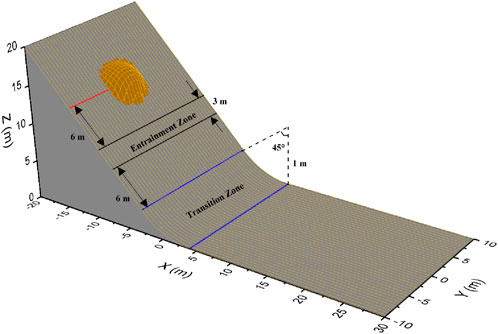
FIGURE 1. Schematic diagram of the flow of a dry granular material over a simple 3D surface.

Simulation results are summarized in Table 1. For comparison, we consider the angle between the initial and final locations of the center of mass (angle of rest, ${\varnothing }_t$). In the ideal case of a frictional rigid block, this angle is equal to the basal friction angle (${\phi }_b$ =25°). In a flow without bed erosion (S1 and S2 in Table 1), the angle is remarkably higher. This difference is due to energy loss caused by the turbulent term of basal resistance (Supplementary Figure S1B of the Supplementary Material), and by the dissipation of kinetic energy during downslope propagation. Greater frictional losses caused by curving path is a source of dissipation. These factors cause the final deposits to stop at shorter distance compared to the rigid block. The stopping distance is even less if we consider bed erosion (S3 and S4 in Table 1), because of the dissipation of kinetic energy during the entrainment process. More detail, volume changes occur as mass is eroded from the bed. Momentum transfer accompanies mass transfer, as material at rest is accelerated to the velocity of the flow by a combination of solid collisions and fluid thrust. This process results in the loss of kinetic energy. Compared to Supplementary Figure S1A of the Supplementary Material, the slope of the energy line in Supplementary Figure S1C of the Supplementary Material is steeper than ${\phi }_b$ because of the energy loss during the collision.

TABLE 1

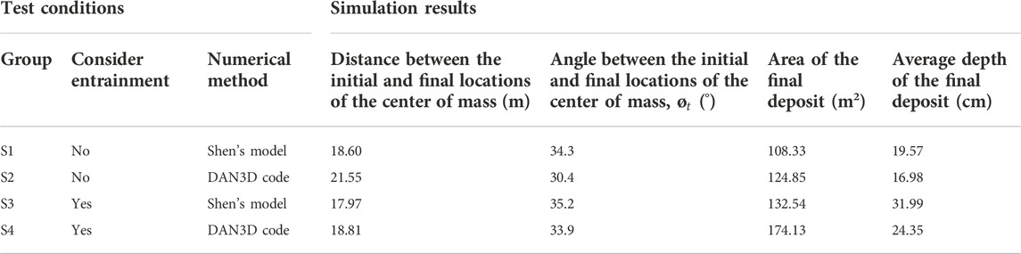
TABLE 1. Test conditions and simulation results.

Deposit of S1 is about 108.33 m² and 19.57 cm in average thickness, while the entrained materials result in a larger deposit area of approximately 132.54 m², with a relatively thicker average depth of approximately 31.99 cm (S3). Similar results appear in the comparison between S2 and S4 as shown in Table 1.

The final deposit characteristics (width, morphology, maximum flow depth, etc.) are shown in Figure 2. As can be seen, different deposit morphologies are predicted by two numerical models. In particular, compared to Shen’s model, a wider and flatter final deposit is provided by the DAN3D model whether the entrainment is considered or not. The most likely reason for this discrepancy is an inherent difference between the two models. According to section 2.1, the equations for determining the stress coefficient are quite different in the two numerical models. Specifically, the method used in Shen’s model tends to apply lower stress in the y-direction, which makes the final deposits exhibit a smaller deposition area and a larger average thickness compared to the DAN3D model.

FIGURE 2

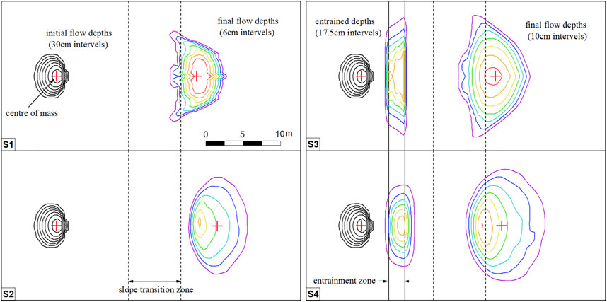
FIGURE 2. Final deposit characteristics of four hypothetical experiments.

Both models reproduce the same entrainment pattern: the entrained depth decreases gradually from the middle to the two sides. But entrainment in DAN3D extends beyond the boundaries of the entrainment zone, which is the result of the SPH-based interpolation method.

The entrainment volume of both models shows in Figure 3A. Entrained materials double the volume after traveling a short distance along the sliding surface. The first and second inflection points represent the start and the end of the entrainment, respectively. The entrainment process lasts approximately 2.5 s, and the total time of motion is about 7.5 s.

FIGURE 3

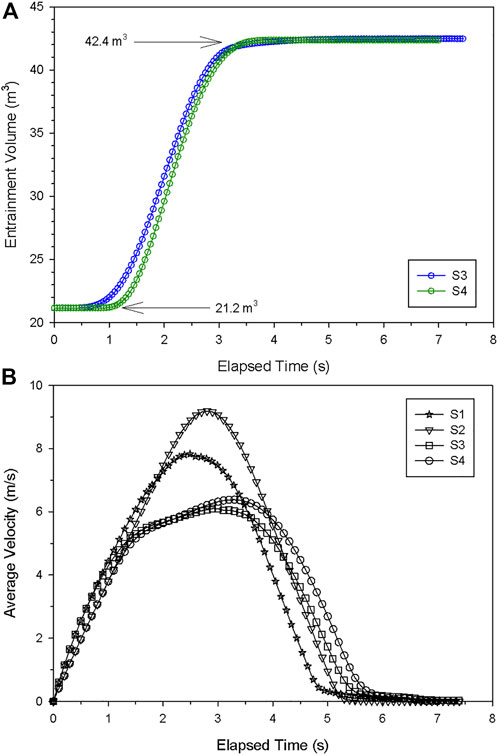
FIGURE 3. Simulated time curves of (A) the entrainment volume and (B) the average velocity of hypothetical experiments.

Figure 3B shows the average velocity of four hypothetical experiments. Under the same simulation condition (no entrainment or entrainment), curves present the same change trend. Particularly, curves S1and S2 contain a steep rising limb and a steep falling limb, while curves S3 and S4 have a relative gentle limb except two limbs mentioned above, which again proves the significant influence of the entrainment on the kinetic energy consumption mentioned above. Besides, the result calculated by the DAN3D code tends to have a higher peak value in both simulation conditions because of the smaller lateral constrains. The lateral constraints herein are referred to the stress exerted by surrounding soil column, which prevent the material from spreading out. Overall, the general agreement between the two codes is to be expected. These simple experiments emphasize both the entrainment and numerical method play a dominant role in dynamic simulation of flow-like slides (morphology of the final deposit).

4 Background of the July 23 debris-flow event

4.1 Study area

The Cancia basin is located in the Borca di Cadore Village (Veneto region, Italy), on the southwestern slope of Mount Antelao (3,264 m a.s.l.). As depicted in Figure 4, the debris-flow channel can be divided into three parts: Part 1 starts from the head of the Salvella basin (2,500 m a.s.l.) and ends at the initiation area (1,665 m a.s.l.) where there is monitoring station (Simoni et al., 2020); Part 2 is the reach from the initiation area to the upper retention basin (1,340 m a.s.l.) which was built in 1996 and progressively enlarged in the autumns of 2009 and 2014; Part 3 starts from the upper retention basin (Figure 4C) and ends at the lower retention basin (1,000 m a.s.l.) as shown in Figure 4D. The channel in Part 1 is incised in the scree deposits with boulders of size up to 8 m (Figure 4A). Part 2 is characterized by relatively narrow cross-sections and a straight channel path, which facilitates the downward propagation of the debris flow. The small retention area at the end of Part 2 stops debris flows of small magnitude and slows down the movement of those of medium-high magnitude. Part 3 contains two sections. The initial 230 m long section was severely eroded due to the high inclination and the water supply from the mouth of the Bus de Diau Creek tributary. The three parts have different slopes, the channel in Part 1 is very steep with a slope of more than 30°, Part 2 has a slope between 20° and 30°, and the first section of Part 3 has a relatively steep slope (20° on average), whereas the second one presents an average slope angle of 14°.

FIGURE 4

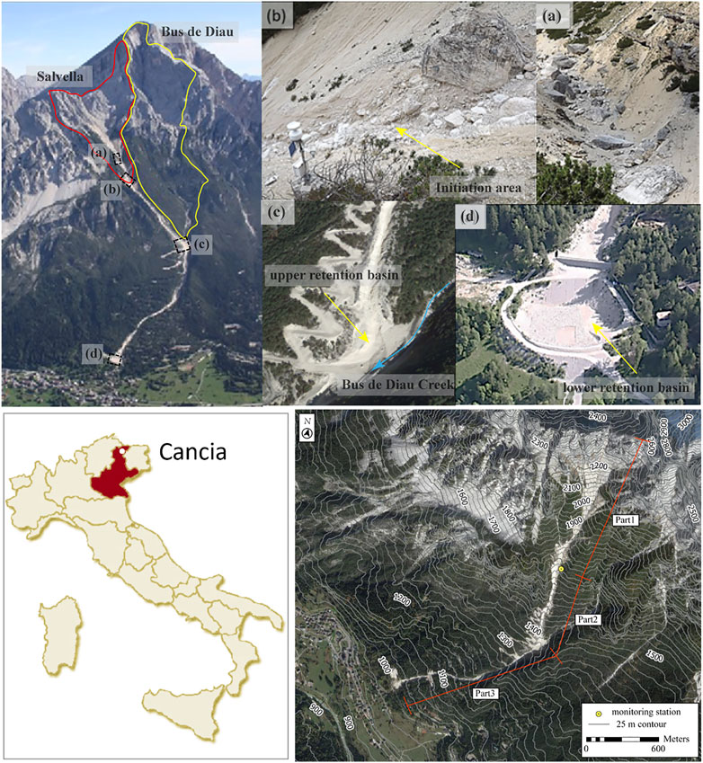
FIGURE 4. General view of the Cancia debris-flow channel and basins (A) the debris flow channel in the upper part of the initiation area; (B) the location of the monitoring station; (C) the upper retention basin at 1,340 m a.s.l.; (D) the lower retention basin at 1,000 m a.s.l.

4.2 Process of the July 23 debris-flow event

The July 23 event is a well-documented debris flow with obvious entrainment (Simoni et al., 2020). At approximately 2:05 p.m. on 23 July 2015, the time-lapse video records the arrival of fast-flowing debris front. Before the event, a short and intense rainfall was with a maximum 5 min rainfall intensity of 106 mm/h (between 2:00 and 2:05 p.m.) was recorded by the rain gauge. The rainwater produced a runoff able to entrain the material in the upper reach of the channel (end of Part 1), thus starting the debris flow. As recorded by the video, the lag time between rainfall onset and debris flow occurrence was 20 min. The front of debris flow was made of boulders and propagated downstream until reached the upper retention basin (end of Part 2) where the solid part of the mixture mostly stopped. Part of the material continued to flow downstream, and finally, the debris flow reached the lower retention basin (end of part 3). On the basis of the field measurements, the total volume of the deposit (28,850 m³) increased significantly compared with the initial volume (around 4,400 m³). Downstream propagation was therefore accompanied by strong entrainment that deepened the channel.

4.3 Entrainment and deposition

For the July 23 event, two topography datasets are available. The first dataset is the LiDAR collected by the Province of Belluno in November 2011, and it is used to derive the pre-event DEM with 1 m resolution. The accuracy of this digital elevation model is uncertain due to the influence of the debris events that occurred in the summer of 2013, as well as the time elapsed from the occurrence of debris flow and the date of data acquisition. For this reason, a GPS-RTK survey carried out in October 2013 and terrestrial laser scanning (TLS) executed in December 2014 were used to locally modify the 2011 LiDAR-derived DEM to acquire a more reliable pre-event DEM (Simoni et al., 2020). The second dataset is a series of aerial photographs taken using UAV technology 8 days after the event. The accuracy of this data is also partially affected by the excavation activities carried out within these 8 days. Post-event DEM were generated from these aerial photographs. The accuracy of pre- and post-event DEMs with 1 m resolution is evaluated through the methodology proposed by Höhle and Höhle (2009) and Höhle and Potuckova (2011).

The map in Supplementary Figure S2 of the Supplementary Material is obtained by comparing pre- and post-event DEM and provides us information about the entrainment and deposition. The total length of the channel is approximately 2,200 m. The topography of the entire channel is modified after the July 23rd debris flow event. The channel from the initiation area to the upper retention basin shows significant entrainment characteristics with a maximum eroded depth exceeding 6 m. Furthermore, the entrainment distribution clearly displays that more materials were entrained in the channel bed while less entrainment occurred in the lateral banks. Deposition zones are mainly distributed in the two retention basins and the relatively gentle area preceding the lower retention basin. More details can be found in Simoni et al. (2020).

5 Simulation results and discussion

5.1 Computational model

Considering both computational efficiency and simulation accuracy, a digital elevation model (DEM) with 2.5 m resolution was resampled from the original DEM with 1 m resolution to generate the 3D computational model (Figure 5A) and the 2D contour map (Figure 5B) before the July 23rd debris flow event. The computational region is 1,600 m in the x direction and 1,387.5 m in the y direction. The minimum and maximum elevations of the simulation area are 945.1 m and 1803.7 m, respectively. This pre-event DEM is used to run simulations, and the post-event DEM was used to validate model results by comparing erosion and deposition areas. According to the field investigations, the entrainment is assumed to cover the entire simulation area.

FIGURE 5

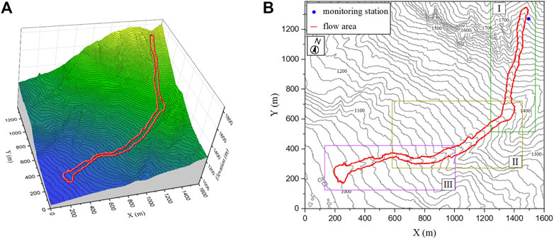
FIGURE 5. (A) A 3D topographic map and (B) a 2D contour map of the simulation area.

5.2 Simulation settings

Two types of simulations were conducted with each model to investigate their performance in case of: i) mass release of the entire debris flow volume in the initiation area and ii) progressive bulking due to entrainment along the channel. The thickness of the erodible layer is set to 8 m for both models. In Shen’s model, the time step increment $∆t$ is calculated by Eq. 17. The maximum time step for simulating this case is 0.005 s in Shen’s model, while a constant time step (0.05s) is set in the DAN3D model.

$∆\mathit{t}\le \mathit{min}\left\{\frac{{\mathit{d}}_{\mathit{x}}}{\mathit{\omega }\mathit{max}\left|{\mathit{v}}_{\mathit{x}}\right|},\frac{{\mathit{d}}_{\mathit{y}}}{\mathit{\omega }\mathit{max}\left|{\mathit{v}}_{\mathit{y}}\right|}\right\}(17)$

Where $\omega$ = 5 is applied in this case. $d_x$ and $d_y$ are the length of grid in the x and y direction, respectively.

The simulation assumptions are listed in Table 2. Simulation C1 and C2 do not consider bed entrainment and simulations C3 and C4 do consider bed entrainment. Calibration of rheological parameters is performed independently for all simulations. In all cases, the final volume is about 29,000 m³, as measured in the field (Simoni et al., 2020). An important difference is that the initial volume is equal to the final one in simulations C1 an C2, where bed entrainment is not taken into account and the whole mass is released in the initiation area, while it is much smaller in simulations C3 and C4 where the volume progressively increases along the channel. In these cases, the entrainment rate was adjusted to reach the measured final volume.

TABLE 2

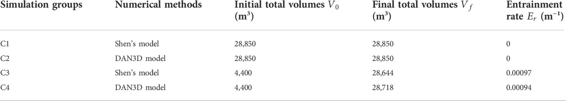
TABLE 2. Setups in different simulation groups.

The physical parameters adopted in these simulations are given in Table 3. Among these parameters, the two Voellmy resistance parameters are determined by trial and error for a good fit in terms of the final flow depth. A default value (35°) is appropriate for dry fragmented rock and 0° for fluids, so the internal friction angle of the debris mass is set to 35°, and the bulk density is set to 2.04 g/cm³.

TABLE 3

TABLE 3. Physical parameters of materials.

5.3 Comparison of the two numerical models

The simulated results of the two models without entrainment are presented in Figure 6. They illustrate that both codes can reasonably simulate the runout process of the debris flow event, by releasing its entire volume in the initiation area. Shen’s model tends to produce greater depositional thickness in the two retention basins compared to the DAN3D code. Meanwhile, the lateral propagation is limited in Shen’s model, which results in a narrower distribution along the simulated flow path. Since the no-entrainment model treats debris flow events as a single surge of large volume, lateral bank overflows were observed in the simulations of the two models while no overflowing occurred along the channel during the actual event (Supplementary Figure S2 of the Supplementary Material). In further detail, the comparison of Figure 6A and Figure 6B shows that the DAN3D model simulates more overbank flows in the upper reach of the channel while Shen’s model mainly overflows further downstream.

FIGURE 6

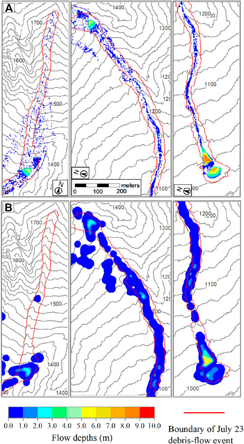
FIGURE 6. Comparison between (A) Shen’s model and (B) DAN3D code in terms of flow depth at end of numerical simulation (The flow depths contours are at 1-m intervals; The elevation contours are at 20-m intervals).

The results obtained by considering the entrainment are shown in Figure 7 as a series of time-lapse images. Figure 7A and Figure 7B show the simulated results using Shen’s model and DAN3D code, respectively. Both models were stopped manually after 750 s (simulated event duration), by which time most of the material had come to rest. Moreover, no further areal development was observed in the subsequent simulation (after 750 s). In order to compare the differences between the two numerical models, we show enlarged details of the simulation results. In Figure 7, significant differences can be observed by comparing the flow depths at the same time steps, especially in the upper (1,340 m a.s.l.) and lower (1,000 m a.s.l.) retention basin. The shape of the inundated area differs for the two models with DAN3D producing a larger lateral spreading along the channel. In the initial phases of the simulated events (t = 50 s and t = 100 s), the travel distance computed by DAN3D is greater compared to Shen’s code, as a consequence of a faster simulated flow. At end of the numerical simulation (t=750 s), DAN3D results show smaller thickness of the deposits but a larger spreading along the entire path, especially at the two retention basins where topography is relatively flat.

FIGURE 7

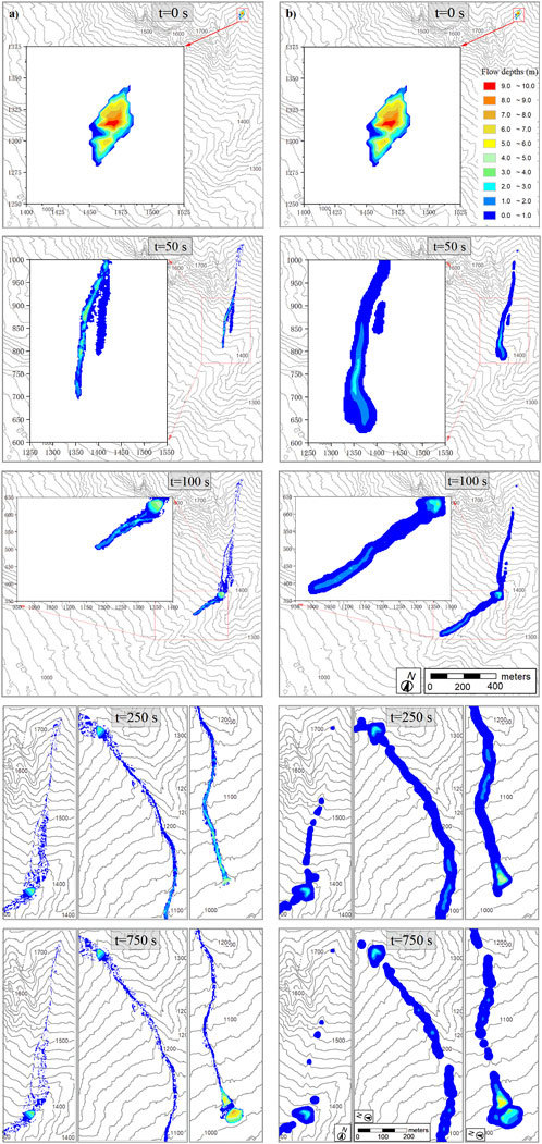
FIGURE 7. Simulated flow depth distributions of (A) Shen’s model and (B) DAN3D model at five selected times (The elevation contours are at 20-m intervals).

Simulation results show that both models can improve their performance in simulating the July 2015 debris flow if debris flow bulking by erosion and entrainment is taken into account (Figure 7). Entrainment, in fact, is a fundamental process characterizing debris flow behavior and simulations without entrainment can only represent a rough approximation (Figure 6). The analysis which includes erosion and entrainment (Figure 7, t=750 s) shows a more satisfactory estimation of the depositional shape compared to the simulation without entrainment. In addition, they allow obtaining more realistic results along the channel with limited to null overflowing episodes, as observed in the field. The Jaccard index was adopted to numerically compare the areal extent between simulations and real events. In simulations accounting for entrainment, Jaccard similarities between simulation and real events are 0.38 (Shen’s model) and 0.54 (DAN3D model), respectively. While in simulations without entrainment, Jaccard similarities of Shen’s and DAN3D models are 0.32 and 0.39, respectively. These primary differences highlight the importance of considering erosion and entrainment in debris flow simulation. In fact, the debris flow was triggered by a short and intense rainfall event that initiated channel erosion just upstream of the monitoring station and that volumetrically grew during its downstream routing (Simoni et al., 2020).

Figure 8 shows that the evolution of the simulated debris flow volume V and average velocity v obtained in the four cases. The simulated results of C3 (28,644 m³) and C4 (28,718 m³) based on the calibrated entrainment rate agree well with the estimated debris flow volume (28,850 m³) in Figure 8A. The differences between two models are not significant. Minor discrepancies in debris flow volume growth are observed. At the beginning, the volume growth of C4 (DAN3D model) is quicker than that of C3 (Shen’s model). However, after about 250 s, the volume growth rate of C3 exceeds C4 until the end of the simulation.

FIGURE 8

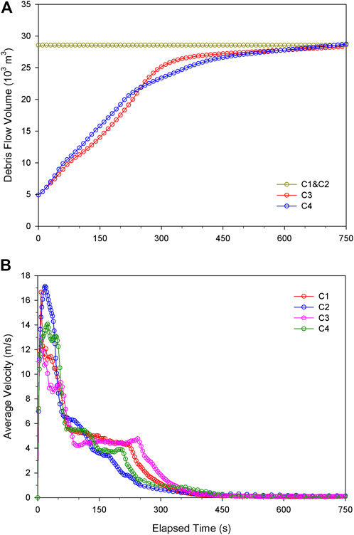
FIGURE 8. Simulated time curves of the (A) debris flow volume and (B) average velocity of the July 23 debris-flow event.

Figure 8B shows that the shape of C1, C2, C3 and C4 is generally similar, but with significant differences. Four key times are marked in four curves to analyze the motion of debris flows in four different simulations. T₁ is the time corresponding to the peak of the curve, t₂ is the end of the first sharp deceleration, t₃ is the start of the second abrupt deceleration, and t₄ represents the moment that the motion of the sliding mass basically stops. From 0 s to t₁, the materials depart from the initiation area and flow along the steep channel. Suddenly, the average velocity drops sharply because the materials reach the region where the channel gradient significantly decreases. At this stage (t₁∼t₂), a minor portion of materials continue to downslope and entrain the additional debris along the path, whereas most of the materials deposit on the upper sediment basin. More specifically, the peak velocities of C1 and C2 are significantly higher than those of C3 and C4. The major reason is that the larger the volume released in the initiation area, the more the associated kinetic energy. Then a slight acceleration is observed for the cases considering the entrainment (C3 and C4) from t₂ to t₃, while this phenomenon does not exist in the cases without the entrainment (C1 and C2). This difference is likely attributed to the mobility increased by the entrained volume. After a progressive deceleration occurring along the lower reach of the channel, the entire motion comes to rest at t₄.

Similar results should be obtained in the two models due to the implementation of the same rheological model and entrainment model. A closer look at the results of the two models, however, reveals some noticeable differences. DAN3D tends to predict a larger and thinner inundated area compared to Shen’s model (Figure 7 and Figure 8B), and the time series of the entrained volume are also different (Figure 8A). Such discrepancies may be due to differences in the numerical scheme, but the complex topography of the channel makes any comparison extremely difficult.

The spatial pattern of erosion simulated by the two numerical models along the debris flow path is reported in Figure 9. It shows the characteristics of entrainment that is more pronounced in the middle section of the flow channel for both models. This erosive character of the flow corresponds to field measures (Supplementary Figure S2 of the Supplementary Material) and is consistent along the channel. Note, in Figure 9B, erosion extends beyond the boundaries of the simulated entrainment zone in some areas downstream of the channel. This discrepancy is due to the use of a meshless interpolation technique based on SPH in the DAN3D code. In this case, when the interpolating kernel W is wider than the grid width (2.5 m), the erodible mass of adjacent grids will be entrained. However, this effect can be neglected at a large-scale simulation because the user-prescribed entrainment zone is not necessarily accurate.

FIGURE 9

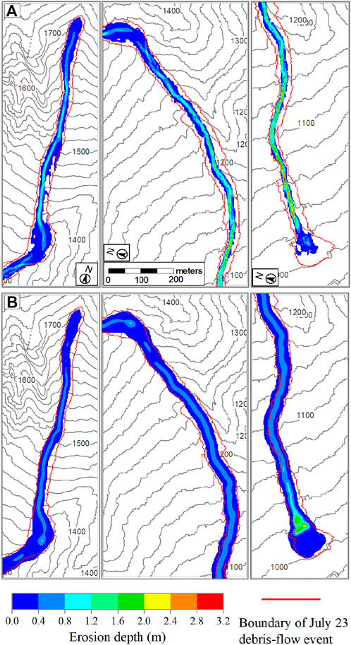
FIGURE 9. The final erosion depths of (A) Shen’s model and (B) DAN3D model.

A detailed comparison between the observed and simulated elevation changes is shown in Figure 10. Overall, there is a reasonable agreement between the field survey and the numerical simulation. All results indicate that the deposition of material mainly occurs in the two retention basins. Other areas exhibit prevailing erosion. However, significant differences are also identified. In the simulations, most of the materials deposit in the lower basin, with a maximum depth of approximately 7.35 m and 4.9 m respectively for the Shen’s model and DAN3D code, respectively. Conversely, in the field investigation, the maximum deposit thickness (7.49 m) was observed in the upper retaining basin rather than the lower basin. Also, as previously mentioned, the DAN3D model produces some overflowing that translates into a larger inundated area along the channel banks.

FIGURE 10

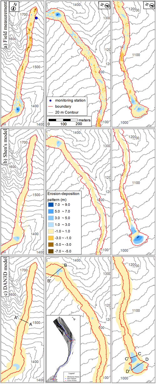
FIGURE 10. The topography changes before and after the debris flow event (A) measured by subtraction of 2.5 m DEMs; (B) calculated by Shen’s model; (C) calculated by DAN3D code.

We selected four different cross-sections (A-A′, B-B′, C-C′ and D-D′ shown in Figure 10C) along the channel to investigate the local significance of the erosion-deposition dynamics (Figure 11). Based of field measures, in section A-A′, erosion deepens the channel bed with a maximum depth of about 6 m. Here, the numerical results also indicate some erosion but with a much lower depth. In section B-B′, both field and numerical results describe the deposition of debris, but the simulation results show a noticeable smaller thickness. Erosion and deposition occur alternately in the following section of the channel down to the lower channel reach where lower gradients are associated to widespread deposition. Here (section C-C′), Shen’s model shows larger thickness of the deposit compared to DAN3D model. Similar to the upper retention basin, abundant sediments fill up the lower basin (section D-D′) with Shen’s model largely overestimating its thickness.

FIGURE 11

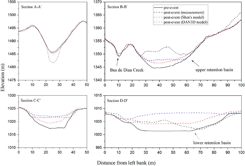
FIGURE 11. Debris flow channel cross-section comparing the pre- and post-event morphology (Section location shown in Figure 10C).

In order to compare the results of the simulations to the actual debris flow event, we reconstruct the slope profile of the study area according to the field topography (Figure 12A), and calculate the yield rate per 20 m along the flow path (Figure 12B). Herein, the concept of yield rate (eroded volume per meter of travel distance) was originally introduced by Hungr et al. (1984) to describe the volume change that occurs when a debris flow moves downward. The average channel slope is 27.2° upstream of the upper retaining basin (1,340 m a.s.l.), and it progressively decreases downslope, with an average value of 12.8°. The red solid line represents the initial sliding mass of the initiation area close to the monitoring station (1,665 m a.s.l.). Figure 12B shows that erosion and deposition are not uniformly distributed along the flow path in both measurement and simulation. Measurements illustrate that erosion dominates in the upper reach of the channel, where the two simulations fail to capture the local peaks of erosion in favor of a more homogeneous pattern distributed along the channel. Further downstream, the negative yield rate describes the deposition of debris, which is higher in the two basins for both measures and simulations. Erosion and deposition alternately occur between the two retention basins both in field observation and the results of the DAN3D code, while there is no deposition in Shen’s model.

FIGURE 12

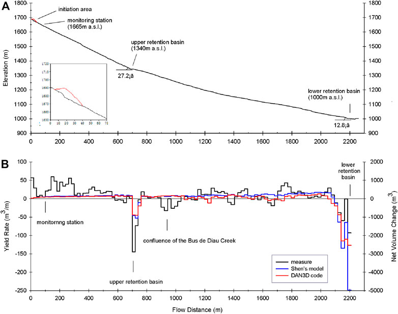
FIGURE 12. Variation of (A) elevation and (B) net volume along the flow distance.

The numerical experiments (section 3) contribute to explain the differences between the two models observed in the case study application. They confirm that the numerical resolution schemes have an impact on the results despite resolution the strong similarities of the two models (rheology, erosion/entrainment models, calibration on the same event, ...). The simulated flows are rather similar in terms of propagation velocity and progressive volume enlargement while the flow inundated area and the thickness of the deposit is significantly different with important impacts on the evaluation of hazard.

6 Conclusion

Two depth-averaged models that include the description of the erosion/entrainment process within debris flows, namely Shen’s model and the DAN3D model, are used to simulate the run-out process of an Alpine debris flow event. The event is well documented allowing for the calibration of erosional and depositional features along the debris flow path in addition to the pattern and thickness of the final deposit. Both models performed reasonably well, giving satisfactory accuracy of the final erosion-deposit distribution, inundation area, and runout distance comparing with the survey measurements. The simulation results highlight the following conclusions.

1) Owing to the peculiar topography of the Cancia debris-flow channel, the motion of the July 23rd event is characterized by two acceleration-deceleration stages. The first stage is dominated by bed erosion and takes place when the materials flow along the upper part of the channel and deposit in the upper retention basin (part 2). The second stage occurs when the materials flow further downstream along the path ending its run in the lower retention basin. The numerical results further emphasize the importance of the topography on the motion of debris flows, highlighting the need of an accurate 3D digital terrain model.

2) Entrainment is a crucial process in reproducing the July 23rd event and, similarly, all debris flows that significantly enlarge their volume during propagation. The simulations that neglect entrainment provide inaccurate results in terms of inundated area, both by exaggerating the final deposit and producing unrealistic channel overflows. Although entrainment is a complex phenomenon, and it is the result of multiple factors, the empirical model adopted in this paper can obtain satisfactory simulation results of entrainment pattern, and an accurate parameter calibration can be performed against experimental field data. However, given simulations acquire greater practical significance when used in predictions, it should be recognized that including entrainment requires a higher number of input parameters that inevitably translate into larger prediction uncertainty.

3) The comparison between observations and simulated results shows that satisfactory agreement can be obtained for the two models considering entrainment. With respect to rheological parameters, separate calibration procedures gave quite similar results, with equal best combination Voellmy resistance parameters ($\tan {\varnothing }_b$ = 0.11 and $\xi$ = 450 m/s²) for the two models. Similarly, the calibrated entrainment rate of both models is quite similar. Such outcomes indicate the robustness of the models. However, the different numerical schemes adopted by the two codes lead to some noticeable differences. For the analyzed case, the DAN3D code always gives higher mobility and larger lateral spreading relative to the Shen model, while Shen’s model reproduces relatively thicker deposits.

Data availability statement

The original contributions presented in the study are included in the article/Supplementary Material, further inquiries can be directed to the corresponding author.

Author contributions

ZQ, TL, WS, and MB conceived the idea of the study. ZQ carried out numerical simulations, prepared the figures, analyzed the results and wrote the manuscript. WS proposed a modified finite difference model for dynamic analysis of flow-like landslides and was responsible for the methodology. AS, CG, and MB participated in the field investigation and acquired substant available field data. TL, AS, CG, WS, and MB were involved in the revision of the manuscript. All authors contribute to the analysis and discussion of the simulation results.

Funding

This research is funded by the National Key R&D Program of China (2021YFE0111900) and the China Scholarship Council (CSC)—University of Bologna Joint Scholarship (File No. 202006560018).

Acknowledgments

We would like to thank the referees for careful reading the manuscript and providing constructive comments to help us improve the quality of this paper.

Conflict of interest

The authors declare that the research was conducted in the absence of any commercial or financial relationships that could be construed as a potential conflict of interest.

Publisher’s note

All claims expressed in this article are solely those of the authors and do not necessarily represent those of their affiliated organizations, or those of the publisher, the editors and the reviewers. Any product that may be evaluated in this article, or claim that may be made by its manufacturer, is not guaranteed or endorsed by the publisher.

Supplementary material

The Supplementary Material for this article can be found online at: https://www.frontiersin.org/articles/10.3389/feart.2022.1059525/full#supplementary-material

References

Abe, K., Johansson, J., and Konagai, K. (2007). A new method for the run-out analysis and motion prediction of rapid and long-traveling landslides with MPM. J. Geotech. Geoenvironmental Eng. 63, 93–109. doi:10.2208/jscejc.63.93

CrossRef Full Text | Google Scholar

Abe, K., and Konagai, K. (2016). Numerical simulation for runout process of debris flow using depth-averaged material point method. Soils Found. 56, 869–888. doi:10.1016/j.sandf.2016.08.011

CrossRef Full Text | Google Scholar

Armanini, A., Fraccarollo, L., and Rosatti, G. (2009). Two-dimensional simulation of debris flows in erodible channels. Comput. Geosci. 35, 993–1006. doi:10.1016/j.cageo.2007.11.008

CrossRef Full Text | Google Scholar

Bao, Y., Chen, J., Sun, X., Han, X., Li, Y., Zhang, Y., et al. (2019). Debris flow prediction and prevention in reservoir area based on finite volume type shallow-water model: A case study of pumped-storage hydroelectric power station site in yi county, hebei, China. Environ. Earth Sci. 78, 577–616. doi:10.1007/s12665-019-8586-4

CrossRef Full Text | Google Scholar

Berti, M., Genevois, R., Simoni, A., and Tecca, P. R. (1999). Field observations of a debris flow event in the Dolomites. Geomorphology 29, 265–274. doi:10.1016/S0169-555X(99)00018-5

CrossRef Full Text | Google Scholar

Berti, M., and Simoni, A. (2014). Dflowz: A free program to evaluate the area potentially inundated by a debris flow. Comput. Geosci. 67, 14–23. doi:10.1016/j.cageo.2014.02.002

CrossRef Full Text | Google Scholar

Blanc, T., Pastor, M., Drempetic, M. S., Drempetic, V., and Haddad, B. (2011). Depth integrated modelling of fast landslide propagation. Eur. J. Environ. Civ. Eng. 15, 51–72. doi:10.1080/19648189.2011.9695304

CrossRef Full Text | Google Scholar

Bollschweiler, M., and Stoffel, M. (2010). Tree rings and debris flows: Recent developments, future directions. Prog. Phys. Geogr. Earth Environ. 34, 625–645. doi:10.1177/0309133310370283

CrossRef Full Text | Google Scholar

Breien, H., De Blasio, F. V., Elverhøi, A., and Høeg, K. (2008). Erosion and morphology of a debris flow caused by a glacial lake outburst flood, Western Norway. Landslides 5, 271–280. doi:10.1007/s10346-008-0118-3

CrossRef Full Text | Google Scholar

Chen, C. L. (1987). Comprehensive review of debris flow modeling concepts in Japan. GSA Rev. Eng. Geol. 7, 13–30. doi:10.1130/REG7-p13

CrossRef Full Text | Google Scholar

Christen, M., Kowalski, J., and Bartelt, P. (2010). Ramms: Numerical simulation of dense snow avalanches in three-dimensional terrain. Cold Reg. Sci. Technol. 63, 1–14. doi:10.1016/j.coldregions.2010.04.005

CrossRef Full Text | Google Scholar

Dai, Z., Huang, Y., Cheng, H., and Xu, Q. (2017). SPH model for fluid–structure interaction and its application to debris flow impact estimation. Landslides 14, 917–928. doi:10.1007/s10346-016-0777-4

CrossRef Full Text | Google Scholar

D’Ambrosio, D., Di Gregorio, S., and Iovine, G. (2003). Simulating debris flows through a hexagonal cellular automata model: SCIDDICA S<sub>3–hex</sub&gt. Nat. Hazards Earth Syst. Sci. 3, 545–559. doi:10.5194/nhess-3-545-2003

CrossRef Full Text | Google Scholar

Damm, B., and Felderer, A. (2013). Impact of atmospheric warming on permafrost degradation and debris flow initiation: A case study from the eastern European Alps. E&amp;amp;G Quat. Sci. J. 62, 136–149. doi:10.3285/eg.62.2.05

CrossRef Full Text | Google Scholar

Draebing, D., and Krautblatter, M. (2019). The efficacy of frost weathering processes in alpine rockwalls. Geophys. Res. Lett. 46, 6516–6524. doi:10.1029/2019GL081981

CrossRef Full Text | Google Scholar

Fraccarollo, L., and Capart, H. (2002). Riemann wave description of erosional dam-break flows. J. Fluid Mech. 461, 183–228. doi:10.1017/S0022112002008455

CrossRef Full Text | Google Scholar

Frank, F., McArdell, B. W., Huggel, C., and Vieli, A. (2015). The importance of entrainment and bulking on debris flow runout modeling: Examples from the Swiss Alps. Nat. Hazards Earth Syst. Sci. 15, 2569–2583. doi:10.5194/nhess-15-2569-2015

CrossRef Full Text | Google Scholar

Frimberger, T., Andrade, S. D., Weber, S., and Krautblatter, M. (2021). Modelling future lahars controlled by different volcanic eruption scenarios at Cotopaxi (Ecuador) calibrated with the massively destructive 1877 lahar. Earth Surf. Process. Landforms 46, 680–700. doi:10.1002/esp.5056

CrossRef Full Text | Google Scholar

Gregoretti, C., Degetto, M., Bernard, M., and Boreggio, M. (2018). The debris flow occurred at ru secco creek, Venetian dolomites, on 4 august 2015: Analysis of the phenomenon, its characteristics and reproduction by models. Front. Earth Sci. 6, 1–20. doi:10.3389/feart.2018.00080

CrossRef Full Text | Google Scholar

Guo, J., Cui, Y., Xu, W., Yin, Y., Li, Y., and Jin, W. (2022). Numerical investigation of the landslide-debris flow transformation process considering topographic and entrainment effects: A case study. Landslides 19, 773–788. doi:10.1007/s10346-021-01791-6

CrossRef Full Text | Google Scholar

Han, Z., Chen, G., Li, Y., Tang, C., Xu, L., He, Y., et al. (2015). Numerical simulation of debris-flow behavior incorporating a dynamic method for estimating the entrainment. Eng. Geol. 190, 52–64. doi:10.1016/j.enggeo.2015.02.009

CrossRef Full Text | Google Scholar

Han, Z., Wang, W., Li, Y., Huang, J., Su, B., Tang, C., et al. (2018). An integrated method for rapid estimation of the valley incision by debris flows. Eng. Geol. 232, 34–45. doi:10.1016/j.enggeo.2017.11.007

CrossRef Full Text | Google Scholar

Höhle, J., and Höhle, M. (2009). Accuracy assessment of digital elevation models by means of robust statistical methods. ISPRS J. Photogramm. Remote Sens. 64, 398–406. doi:10.1016/j.isprsjprs.2009.02.003

CrossRef Full Text | Google Scholar

Höhle, J., and Potuckova, M. (2011). Assessment of the quality of digital terrain medels. Off. Publ. - EuroSDR.

Google Scholar

Hungr, O. (1995). A model for the runout analysis of rapid flow slides, debris flows, and avalanches. Can. Geotech. J. 32, 610–623. doi:10.1139/t95-063

CrossRef Full Text | Google Scholar

Hungr, O., Evans, S. G., Bovis, M. J., and Hutchinson, J. N. (2001). A review of the classification of landslides of the flow type. Environ. Eng. Geosci. 7, 221–238. doi:10.2113/gseegeosci.7.3.221

CrossRef Full Text | Google Scholar

Hungr, O., Morgan, G. C., and Kellerhals, R. (1984). Quantitative analysis of debris torrent hazards for design of remedial measures. Can. Geotech. J. 21, 663–677. doi:10.1139/t84-073

CrossRef Full Text | Google Scholar

Hutter, K., Svendsen, B., and Rickenmann, D. (1996). Debris flow modeling: A review. Contin. Mech. Thermodyn. 8, 1–35. doi:10.1007/BF01175749

CrossRef Full Text | Google Scholar

Iverson, R. M. (2012). Elementary theory of bed-sediment entrainment by debris flows and avalanches. J. Geophys. Res. 117, 1–17. doi:10.1029/2011JF002189

CrossRef Full Text | Google Scholar

Iverson, R. M., and Ouyang, C. (2015). Entrainment of bed material by Earth-surface mass flows: Review and reformulation of depth-integrated theory. Rev. Geophys. 53, 27–58. doi:10.1002/2013RG000447

CrossRef Full Text | Google Scholar

Jakob, M., and Hungr, O. (2005). “Introduction,” in Debris-flow hazards and related phenomena (Berlin, Germany: Springer), 1–7.

Google Scholar

Kazmi, Z. A., Konagai, K., and Ikeda, T. (2014). Field measurements and numerical simulation of debris flows from dolomite slopes destabilized during the 2005 Kashmir earthquake, Pakistan. J. Earthq. Eng. 18, 364–388. doi:10.1080/13632469.2013.873372

CrossRef Full Text | Google Scholar

Kazmi, Z. A., Konagai, K., and Ikeda, T. (2012). “Physical and numerical study of debris flows from dolomite slopes exposed in the 2005 kashmir earthquake, Pakistan,” in Proceedings of the 15th World Conf. Earthq. Eng, Lisbon, Portugal, 24-28 September 2012.

Google Scholar

Li, X., Yan, Q., Zhao, S., Luo, Y., Wu, Y., and Wang, D. (2020). Investigation of influence of baffles on landslide debris mobility by 3D material point method. Landslides 17, 1129–1143. doi:10.1007/s10346-020-01346-1

CrossRef Full Text | Google Scholar

Lin, C., Pastor, M., Yague, A., Tayyebi, S. M., Stickle, M. M., Manzanal, D., et al. (2019). A depth-integrated SPH model for debris floods: Application to Lo Wai (Hong Kong) debris flood of August 2005. Geotechnique 69, 1035–1055. doi:10.1680/jgeot.17.P.267

CrossRef Full Text | Google Scholar

McDougall, S. (2006). A new continuum dynamic model for the analysis of extremely rapid landslide motion across complex 3D terrain. PhD thesis. Vancouver (BC): University of British Columbia. doi:10.14288/1.0052928

CrossRef Full Text | Google Scholar

McDougall, S., and Hungr, O. (2004). A model for the analysis of rapid landslide motion across three-dimensional terrain. Can. Geotech. J. 41, 1084–1097. doi:10.1139/T04-052

CrossRef Full Text | Google Scholar

McDougall, S., and Hungr, O. (2005). Dynamic modelling of entrainment in rapid landslides. Can. Geotech. J. 42, 1437–1448. doi:10.1139/t05-064

CrossRef Full Text | Google Scholar

Medina, V., Hürlimann, M., and Bateman, A. (2008). Application of FLATModel, a 2D finite volume code, to debris flows in the northeastern part of the Iberian Peninsula. Landslides 5, 127–142. doi:10.1007/s10346-007-0102-3

CrossRef Full Text | Google Scholar

Mousavi Tayebi, S. A., Moussavi Tayyebi, S., and Pastor, M. (2021). Depth-integrated two-phase modeling of two real cases: A comparison between r.avaflow and geoflow-sph codes. Appl. Sci. (Basel). 11, 5751. doi:10.3390/app11125751

CrossRef Full Text | Google Scholar

O’Brien, J. S., Julien, P. Y., and Fullerton, W. T. (1993). Two-Dimensional water flood and mudflow simulation. J. Hydraul. Eng. 119, 244–261. doi:10.1061/(asce)0733-9429(1993)119:2(244)

CrossRef Full Text | Google Scholar

Ouyang, C., He, S., and Tang, C. (2015). Numerical analysis of dynamics of debris flow over erodible beds in Wenchuan earthquake-induced area. Eng. Geol. 194, 62–72. doi:10.1016/j.enggeo.2014.07.012

CrossRef Full Text | Google Scholar

Ouyang, C., He, S., Xu, Q., Luo, Y., and Zhang, W. (2013). A MacCormack-TVD finite difference method to simulate the mass flow in mountainous terrain with variable computational domain. Comput. Geosci. 52, 1–10. doi:10.1016/j.cageo.2012.08.024

CrossRef Full Text | Google Scholar

Pastor, M., Blanc, T., Haddad, B., Drempetic, V., Morles, M. S., Dutto, P., et al. (2015). Depth averaged models for fast landslide propagation: Mathematical, rheological and numerical aspects. Arch. Comput. Methods Eng. 22, 67–104. doi:10.1007/s11831-014-9110-3

CrossRef Full Text | Google Scholar

Pastor, M., Blanc, T., Haddad, B., Petrone, S., Sanchez Morles, M., Drempetic, V., et al. (2014). Application of a SPH depth-integrated model to landslide run-out analysis. Landslides 11, 793–812. doi:10.1007/s10346-014-0484-y

CrossRef Full Text | Google Scholar

Pastor, M., Haddad, B., Sorbino, G., Cuomo, S., and Drempetic, V. (2009). A depth-integrated, coupled SPH model for flow-like landslides and related phenomena. Int. J. Numer. Anal. Methods Geomech. 30, 1303–1336. doi:10.1002/nag

CrossRef Full Text | Google Scholar

Pirulli, M. (2005). Numerical modelling of landslides runOut. PhD thesis. Turin (TO): Polytechnic University of Turin.

Google Scholar

Pirulli, M., and Pastor, M. (2012). Numerical study on the entrainment of bed material into rapid landslides. Geotechnique 62, 959–972. doi:10.1680/geot.10.P.074

CrossRef Full Text | Google Scholar

Pudasaini, S. P., and Fischer, J. T. (2020). A mechanical erosion model for two-phase mass flows. Int. J. Multiph. Flow 132, 103416. doi:10.1016/j.ijmultiphaseflow.2020.103416

CrossRef Full Text | Google Scholar

Rengers, F. K., McGuire, L. A., Oakley, N. S., Kean, J. W., Staley, D. M., and Tang, H. (2020). Landslides after wildfire: Initiation, magnitude, and mobility. Landslides 17, 2631–2641. doi:10.1007/s10346-020-01506-3

CrossRef Full Text | Google Scholar

Sassa, K. (1988). “Geotechnical model for the motion of land-slides,” in Proceedings of the 5th International Symposium on landslides, Lausanne, Switzerland, 10-15 July 1988, 37–55.

Google Scholar

Sassa, K., Nagai, O., Solidum, R., Yamazaki, Y., and Ohta, H. (2010). An integrated model simulating the initiation and motion of earthquake and rain induced rapid landslides and its application to the 2006 Leyte landslide. Landslides 7, 219–236. doi:10.1007/s10346-010-0230-z

CrossRef Full Text | Google Scholar

Sauthier, C., Pirulli, M., Pisani, G., Scavia, C., and Labiouse, V. (2015). Numerical modelling of gravel unconstrained flow experiments with the DAN3D and RASH3D codes. Comput. Geosci. 85, 81–90. doi:10.1016/j.cageo.2015.09.008

CrossRef Full Text | Google Scholar

Savage, S. B., and Hutter, K. (1989). The motion of a finite mass of granular material down a rough incline. J. Fluid Mech. 199, 177–215. doi:10.1017/S0022112089000340

CrossRef Full Text | Google Scholar

Shen, W., Berti, M., Li, T., Benini, A., and Qiao, Z. (2022). The influence of slope gradient and gully channel on the run-out behavior of rockslide-debris flow: An analysis on the verghereto landslide in Italy. Landslides 19, 885–900. doi:10.1007/s10346-022-01848-0

CrossRef Full Text | Google Scholar

Shen, W., Li, T., Li, P., Berti, M., Shen, Y., and Guo, J. (2019). A two-layer numerical model for simulating the frontal plowing phenomenon of flow-like landslides. Eng. Geol. 259, 105168. doi:10.1016/j.enggeo.2019.105168

CrossRef Full Text | Google Scholar

Shen, W., Li, T., Li, P., and Guo, J. (2018). A modified finite difference model for the modeling of flowslides. Landslides 15, 1577–1593. doi:10.1007/s10346-018-0980-6

CrossRef Full Text | Google Scholar

Simoni, A., Bernard, M., Berti, M., Boreggio, M., Lanzoni, S., Stancanelli, L. M., et al. (2020). Runoff-generated debris flows: Observation of initiation conditions and erosion–deposition dynamics along the channel at Cancia (eastern Italian Alps). Earth Surf. Process. Landforms 45, 3556–3571. doi:10.1002/esp.4981

CrossRef Full Text | Google Scholar

Sovilla, B., Burlando, P., and Bartelt, P. (2006). Field experiments and numerical modeling of mass entrainment in snow avalanches. J. Geophys. Res. 111, 1–16. doi:10.1029/2005JF000391

PubMed Abstract | CrossRef Full Text | Google Scholar

Stoffel, M., Mendlik, T., Schneuwly-Bollschweiler, M., and Gobiet, A. (2014). Possible impacts of climate change on debris-flow activity in the Swiss Alps. Clim. Change 122, 141–155. doi:10.1007/s10584-013-0993-z

CrossRef Full Text | Google Scholar

Takahashi, T. (2014). Debris flow: Mechanics, prediction and countermeasures. 2nd ed. Balkema: CRC Press. doi:10.1146/annurev.fl.13.010181.000421

CrossRef Full Text | Google Scholar

Vagnon, F., Pirulli, M., Yague, A., and Pastor, M. (2019). Comparison of two depth-averaged numerical models for debris flow runout estimation. Can. Geotech. J. 56, 89–101. doi:10.1139/cgj-2017-0455

CrossRef Full Text | Google Scholar

Vicari, H., Tran, Q. A., Nordal, S., and Thakur, V. (2022). MPM modelling of debris flow entrainment and interaction with an upstream flexible barrier. Landslides 19, 2101–2115. doi:10.1007/s10346-022-01886-8

CrossRef Full Text | Google Scholar

Voellmy, A. (1955). Über die Zerstörungskraft von Lawinen. Schweiz. Bauztg. 73, 212–285.

Google Scholar

Wang, L., Zhang, X., Lei, Q., Panayides, S., and Tinti, S. (2022). A three-dimensional particle finite element model for simulating soil flow with elastoplasticity. Acta Geotech. 1, 5639–5653. doi:10.1007/s11440-022-01618-1

PubMed Abstract | CrossRef Full Text | Google Scholar

Wang, W., Chen, G., Han, Z., Zhou, S., Zhang, H., and Jing, P. (2016). 3D numerical simulation of debris-flow motion using SPH method incorporating non-Newtonian fluid behavior. Nat. Hazards 81, 1981–1998. doi:10.1007/s11069-016-2171-x

CrossRef Full Text | Google Scholar

Wang, Z., and Shen, H. (1999). Lagrangian simulation of one-dimensional dam-break flow. J. Hydraul. Eng. 125, 1217–1220. doi:10.1061/(asce)0733-9429(1999)125:11(1217)

CrossRef Full Text | Google Scholar

Wieland, M., Gray, J. M. N. T., and Hutter, K. (1999). Channelized free-surface flow of cohesionless granular avalanches in a chute with shallow lateral curvature. J. Fluid Mech. 392, 73–100. doi:10.1017/s0022112099005467

CrossRef Full Text | Google Scholar

Wu, Y., and Lan, H. (2020). Debris flow analyst (da): A debris flow model considering kinematic uncertainties and using a gis platform. Eng. Geol. 279, 105877. doi:10.1016/j.enggeo.2020.105877

CrossRef Full Text | Google Scholar

Zhang, X., Wang, L., Krabbenhoft, K., and Tinti, S. (2020). A case study and implication: Particle finite element modelling of the 2010 saint-jude sensitive clay landslide. Landslides 17, 1117–1127. doi:10.1007/s10346-019-01330-4

CrossRef Full Text | Google Scholar

Zhang, Y., Chen, J., Tan, C., Bao, Y., Han, X., Yan, J., et al. (2021). A novel approach to simulating debris flow runout via a three-dimensional CFD code: A case study of xiaojia gully. Bull. Eng. Geol. Environ. 80, 5293–5313. doi:10.1007/s10064-021-02270-x

CrossRef Full Text | Google Scholar