Evolutionary mechanisms of the strong winds associated with an intense cold wave event and their effects on the wind power production

Cold wave events (CWEs) often cause major economic losses and serious casualties in the cold seasons, making CWEs among the most significant types of disastrous weather. Previous studies have mainly focused on disasters due to abrupt drops in surface temperatures, with less discussion of the strong winds associated with CWEs. Based on an intense CWE that occurred in late December 2020, we investigated the evolutionary mechanisms of the associated strong winds in terms of kinetic energy (KE) budget and evaluated the effects of this CWE on wind power production based on quantitative comparisons with the mean state. The results showed that the CWE occurred under favorable background conditions, which were characterized by a southward-moving transversal trough and a southeastward-moving shortwave trough in the middle troposphere. The surface high ridge that formed around Lake Baikal and the cold front around the southern periphery of the ridge were key factors related to the CWE evolution. The positive work carried out on the horizontal wind by the pressure gradient force that linked a lower tropospheric high-pressure ridge inland and a low-pressure trough offshore and the downward momentum transportation due to the descending motions behind the cold front dominated the enhancement and sustainment of the CWE-associated strong winds. The CWE contributed to wind power production by 1) increasing the wind power density (by an average of ∼1.05-fold) and 2) improving the availability of the wind to generate power, as it reduced the percentage of zero wind power generation by ∼6.4%, while maintaining the high-wind-velocity cut-out percentage.

1 Introduction

The American Meteorological Society defines a cold wave event (CWE) as a rapid fall in temperature within 24 h to temperatures requiring substantially increased protection to agriculture, industry, commerce, and social activities (https://glossary.ametsoc.org/wiki/Cold_wave). In China, the threshold for a CWE is usually a temperature decrease of 10°C in 48 h and a minimum temperature of 4°C (Qian and Zhang, 2007; Fu et al., 2012). CWEs are often called “weather whiplashes”, as they are characterized by an abrupt shift in the daily surface temperature, which can freeze vegetables, induce crop dormancy, catch people off guard, and cause notable injury or other health impacts, in addition to serious property and infrastructure damage and losses(IPCC, 2012; Ma and Zhu, 2020). At the middle and high latitudes of the Northern Hemisphere, CWEs are among the most important types of disastrous weather in the cold season (Cattiaux et al., 2010; Geert et al., 2019). In the context of global warming, the winter surface air temperatures over mid-latitudes tend to be lower (Qian et al., 2019; Zhang et al., 2021), which may increase CWE frequency and enhance the intensity of their associated disasters (Cattiaux et al., 2010; Cohen et al., 2014; Ma and Zhu, 2020; Mu et al., 2022).

In addition to damage due to the rapid chilling, strong winds are another important type of disaster associated with CWEs (Qian and Zhang, 2007; Fu et al., 2012; Bueh et al., 2022). A 46-year statistical study by Qian and Zhang (2007) reported a wide range of CWE-associated strong winds in China, with a mean annual frequency of 20–70 days. These strong winds usually featured a mean velocity of 8–13.8 m s⁻¹, with ∼10% of them reaching velocities of 13.9–20.7 m s⁻¹. In one extreme CWE that affected northern Inner Mongolia, an instantaneous wind speed >40 m s⁻¹ was observed, thus demonstrating the destructive power of such strong winds. Although the strong winds associated with CWEs have produced serious disasters in China, with notable economic losses and casualties (Fu et al., 2012), few studies have focused on the formation mechanisms of CWEs. Therefore, key processes that produce strong winds associated with CWEs remain unknown.

When CWEs occur, as the surface temperature lowers sharply (Zhang et al., 2021), the heating energy consumption increases, particularly in developed regions (Jiang et al., 2018). As strong winds are a key feature CWEs (Qian and Zhang, 2007; Fu et al., 2012), the additional energy consumption can be entirely or partly offset by the electricity generated from wind turbines (Yuan, 2016). Furthermore, using more wind power to replace conventional energy resources (e.g., fuel/oil) can lower the environmental impacts due to carbon emission, which contributes to reaching climate targets (Cherp et al., 2021; Pryor, et al., 2021). The effective use of the wind power associated with CWEs requires detailed evaluations of the energy features of the strong winds. However, previous studies have not often discussed CWE-associated wind energy, and the key features remain unclear.

In late December 2020, China experienced a serious CWE (Figure 1; Mu et al., 2022; Bueh et al., 2022). During this event, the surface temperatures measured at 20 national meteorological stations reached or fell below their respective local historical low temperatures for December (Bueh et al., 2022). Among these, the observed temperatures at the Taiyuan (Shanxi Province) and Hengshan (Hunan Province) stations dropped to –20.6°C and –15.9°C, respectively, breaking their record lowest temperatures (Bueh et al., 2022; Mu et al., 2022). This CWE affected ∼70% of the territory of China: in the early morning of December 31, 2020, the CWE reached its largest range, with the 0°C isotherm located around 25 ^oN (Figure 1I), south of the Yangtze River. During this CWE, strong winds rushed from north to south/southeast (Figure 1), with heavy snowfall mainly in Mongolia, Russia, and Central China (Figure 2). The present study selected this typical CWE to address the following scientific questions: 1) what are the key weather systems and governing mechanisms that produce CWE-associated strong winds (mainly strong winds <850 hPa, as they are most closely related to human society)? 2) How do CWE-associated strong winds affect wind power production? The results are helpful to fill the knowledge gaps aforementioned. The remainder of this report is structured as follows: Section 2 describes the data and methods used in this study, the main results are shown in Sections 3 and Sections 4, and the conclusions and discussion are provided in Section 5.

FIGURE 1

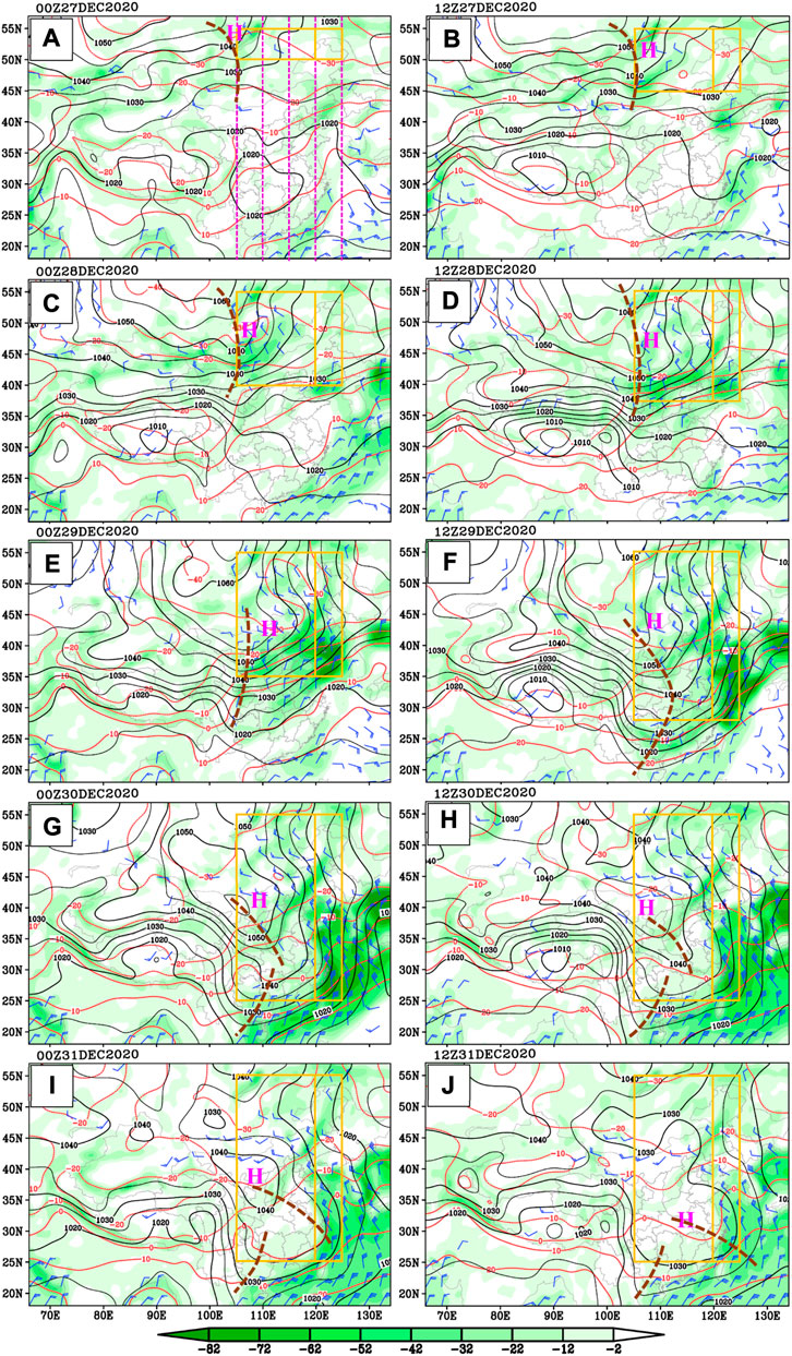
FIGURE 1. Temperature (red contours; °C), temperature advection (shading; 10⁻⁵ K s⁻¹), and wind >4 m s⁻¹ (full bar = 4 m s⁻¹) at surface and sea level pressures (black contours; hPa) ‘H’ = high ridge. Brown dashed lines = locations of ridge lines. Thin dashed purple lines = B1 and B2 notably affected by the cold wave event. Yellow boxes = FR1 and FR2 of the cold wave event.

FIGURE 2

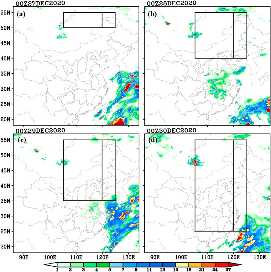
FIGURE 2. 24-hour accumulated precipitation (shading; mm) during the cold wave event. Black boxes = FR1 and FR2 of the cold wave event.

2 Data and methods

2.1 Data

This study utilized two types of data: 1)hourly, 0.25° × 0.25° European Centre for Medium-Range Weather Forecasts (ECMWF) Reanalysis Fifth-Generation (ERA5; Hersbach et al., 2020) data at certain pressure levels (37 vertical levels), heights of 100-m/10-m/2-m above ground level (AGL) and the surface were used for synoptic analyses and quantitative calculations (including three-dimensional wind, temperature, geopotential, relative humidity, sea level pressure, surface wind, surface temperature, and wind at 100 m); and 2)daily, 0.1°×0.1° GPM IMERG final precipitation data (Huffman et al., 2019) for precipitation analysis.

2.2 Methods and key parameters

This study mainly analyzed CWE-associated strong winds in terms of kinetic energy (KE). The basic equations for atmospheric motion under the pressure coordinate were as follows (Holton, 2004):

$\frac{\partial \mathit{u}}{\partial \mathit{t}}=-\mathit{u}\frac{\partial \mathit{u}}{\partial \mathit{x}}-\mathit{v}\frac{\partial \mathit{u}}{\partial \mathit{y}}-\mathit{\omega }\frac{\partial \mathit{u}}{\partial \mathit{p}}-\frac{\partial \mathit{\Phi }}{\partial \mathit{x}}+\mathit{f}\mathit{v}+{\mathit{D}}_{\mathit{x},}(1)$

$\frac{\partial \mathit{v}}{\partial \mathit{t}}=-\mathit{u}\frac{\partial \mathit{v}}{\partial \mathit{x}}-\mathit{v}\frac{\partial \mathit{v}}{\partial \mathit{y}}-\mathit{\omega }\frac{\partial \mathit{v}}{\partial \mathit{p}}-\frac{\partial \mathit{\Phi }}{\partial \mathit{y}}-\mathit{f}\mathit{u}+{\mathit{D}}_{\mathit{y},}(2)$

where u and v are the zonal and meridional winds, respectively; t is time; p is pressure; ω is the vertical velocity in the pressure coordinate; Φ is the geopotential; f is the Coriolis parameter; and D_x and D_y are the friction force in the x and y directions, respectively. We calculated the result of u*Eq. 1 + v* Eq. 2 to obtain Eq. 3:

$\frac{\partial {(\mathit{u}}^{\mathbf{2}}+{\mathit{v}}^{\mathbf{2}})/\mathbf{2}}{\partial \mathit{t}}=-\mathit{u}\frac{\partial {(\mathit{u}}^{\mathbf{2}}+{\mathit{v}}^{\mathbf{2}})/\mathbf{2}}{\partial \mathit{x}}-\mathit{v}\frac{\partial {(\mathit{u}}^{\mathbf{2}}+{\mathit{v}}^{\mathbf{2}})/\mathbf{2}}{\partial \mathit{y}}-\mathit{\omega }\frac{\partial {(\mathit{u}}^{\mathbf{2}}+{\mathit{v}}^{\mathbf{2}})/\mathbf{2}}{\partial \mathit{p}}-\mathit{u}\frac{\partial \mathit{\Phi }}{\partial \mathit{x}}-\mathit{v}\frac{\partial \mathit{\Phi }}{\partial \mathit{y}}+{\mathit{u}\mathit{D}}_{\mathit{x}}+\mathit{v}{\mathit{D}}_{\mathit{y}}.(3)$

The KE of the horizontal wind is defined as ${\mathit{k}}_{\mathrm{h}}={(\mathit{u}}^{\mathbf{2}}+{\mathit{v}}^{\mathbf{2}})/\mathbf{2}$, where the subscript ‘h’ denotes the horizontal component (Fu et al., 2013, 2016); and the work of friction force as ${\mathrm{W}\mathrm{F}=\mathit{u}\mathit{D}}_{\mathit{x}}+\mathit{v}{\mathit{D}}_{\mathit{y}}$, Eq. 3 can be rewritten as follows:

$\frac{\partial {\mathit{k}}_{\mathrm{h}}}{\partial \mathit{t}}=-\mathit{u}\frac{\partial {\mathit{k}}_{\mathrm{h}}}{\partial \mathit{x}}-\mathit{v}\frac{\partial {\mathit{k}}_{\mathrm{h}}}{\partial \mathit{y}}-\mathbf{\omega }\frac{\partial {\mathit{k}}_{\mathrm{h}}}{\partial \mathit{p}}-\mathit{u}\frac{\partial \mathbf{\Phi }}{\partial \mathit{x}}-\mathit{v}\frac{\partial \mathbf{\Phi }}{\partial \mathit{y}}+\mathrm{W}\mathrm{F}.(4)$

Based on the hourly ERA5 reanalysis data, the present study calculated the KE budgets by using Eq. 4 to investigate the KE features and formation mechanisms of the strong winds associated with the CWE. The physical significances of Eq. 4 were as follows: term $\partial {\mathit{k}}_{\mathrm{h}}/\partial \mathbf{t}$ indicates the local temporal variation in KE (LTV), which was calculated using the central difference scheme (Fu et al., 2016, 2019); terms $-\mathit{u}\partial {\mathit{k}}_{\mathrm{h}}/\partial \mathit{x}$ and $-\mathit{v}\partial {\mathit{k}}_{\mathrm{h}}/\partial \mathit{y}$ indicate the zonal wind advection (ZWA) and meridional wind advection (MWA) of the KE, respectively; term $-\mathbf{\omega }\partial {\mathit{k}}_{\mathrm{h}}/\partial \mathit{p}$ represents the vertical advection of the KE (VAD); and terms $-\mathit{u}\partial \mathit{\Phi }/\partial \mathit{x}$ and $-\mathit{v}\partial \mathit{\Phi }/\partial \mathit{y}$ are the pressure gradient force work on zonal wind (WZW) and meridional wind (WMW), respectively. The total effect term (TOT) was defined as TOT=ZWA+MWA+VAD+WZW+WMW to represent the sum of all terms on the right-hand side of Eq. 4 except for the WF.

2.3 Key parameters

Since the range of the CWE changed with time, in this study, we defined two focus regions (FRs; yellow boxes in Figure 1; the one on the left/right side was defined as FR1/FR2) to investigate the strong winds during the CWE. Detailed information about the definition was as follows: 1) as the purple dashed lines in Figure 1A show, central and eastern China could be divided evenly into four bands: 105–110°E, 110–115°E, 115–120°E, and 120–125°E, where the CWE exerted notable influences. As the respective zonal means within the bands of 105–110°E, 110–115°E, and 115–120°E were similar (not shown), we used the zonal mean within the band of 105–120°E (defined as B1) to represent the overall inland features of the CWE. The features of the band at 120–125°E (defined as B2) differed from those of B1 since it was mainly located offshore in the latitudes of 20–40°N. We did not focus on the regions west of 105°E and east of 125°E, as the Tibetan Plateau, which has a mean height of 4,000 m, occupied a large proportion of the former, while the latter was mainly located over the sea. Therefore, the western boundary line of FR1 and the eastern boundary line of FR2 were located at 105°E and 125°E, respectively. 2) The northern boundary line of the FRs was at 55°N, as it was within the source region of the CWE. We did not analyze the regions north of 55°N. The southern boundary lines of the FRs (yellow boxes in Figure 1) were defined as the latitudes (at 1° intervals) where the maximum surface winds associated with the CWE appeared (when the wind speed was the same at two latitudes, we used the larger latitude, which was closer to the source region of the CWE). As the plotting of the wind barbs in Figure 1 used a skipping of 10 grids to keep clarity, the FRs could not be determined by the wind barbs illustrated in Figure 1; instead, we used the grid values of the surface winds (at a resolution of 0.25°×0.25°) to determine the location of the FRs. 3) To compare the different features within the regions inland and offshore, FR1 and FR2 were defined, which were separated by the longitude of 120^oE (FR1/FR2 was located within B1/B2). As the CWE enlarged to the sea, the features within FR2 were used to represent offshore features of the CWE.

The wind power density (WPD), which represents the number of watts of electrical energy produced per square meter of air space (Gualtieri et al., 2021), was calculated at the height of 100 m AGL (a height close to that of the wind turbine) the following equation (Aboobacker et al., 2021; Wen et al., 2021):

$\mathbf{W}\mathbf{P}\mathbf{D}=\frac{\mathit{\rho }{\mathit{V}}^{\mathbf{3}}}{\mathbf{2}},(5)$

where ρ is the air density and V is wind speed. In the present study, we calculated ρ as $\mathbf{\rho }=\mathit{p}/{\mathit{R}}_{\mathit{d}}{\mathit{T}}_{\mathit{v}}$ rather than using a constant value, where R_d and T_v are the gas constant for dry air and the virtual temperature, respectively (Holton, 2004).

As the wind turbine can only work normally at wind speeds between 3 m s⁻¹ and 25 m s⁻¹, we defined the “percentage of zero wind power generation due to low wind velocity” as ${\mathit{P}}_{\mathbf{L}}={\mathit{N}}_{\mathbf{L}}/{\mathit{N}}_{\mathbf{T}}$, where ${\mathit{N}}_{\mathbf{L}}$ was the number of hours that the wind speed was <3 m s⁻¹ and ${\mathit{N}}_{\mathbf{T}}$ was the total number of hours of the evaluation period. Similarly, we defined the “high-wind-velocity cut-out percentage” as ${\mathit{P}}_{\mathbf{H}}={\mathit{N}}_{\mathbf{H}}/{\mathit{N}}_{\mathbf{T}}$, where ${\mathit{N}}_{\mathbf{H}}$ was the number of hours that the wind speed was >25 m s⁻¹. While the lower and upper speed limits might be changed in the future, the calculation methods of the two percentages would stay the same.

To compare the WPD in the mean state to that during the CWE, we defined the increasing ratio as $\mathbf{I}\mathbf{R}=\left({\mathbf{W}\mathbf{P}\mathbf{D}}_{\mathbf{C}}-{\mathbf{W}\mathbf{P}\mathbf{D}}_{\mathbf{M}}\right)/{\mathbf{W}\mathbf{P}\mathbf{D}}_{\mathbf{M}}$, where ${\mathbf{W}\mathbf{P}\mathbf{D}}_{\mathbf{C}}$ is the temporal mean of the WPD during the CWE and ${\mathbf{W}\mathbf{P}\mathbf{D}}_{\mathbf{M}}$ is the temporal mean of the WPD during a long period, which reflects the mean state (i.e., the present study used the period of five consecutive winters from 2016 to 2020).

3 Overview of the cold wave event and synoptic analyses

At 0000 UTC on December 27, 2020, a surface high ridge was maintained around Lake Baikal (‘H’ in Figure 1A), with snowfall to the southwest (Figure 2A). The surface temperature in the central region of the ridge was below -30°C, providing strong cold air for the CWE. Over the surface ridge was a middle-level transversal trough, with a rapidly southeastward-moving shortwave trough (defined as T2) located to its southwest. Strong northwesterly winds occurred ahead of T2, providing favorable conditions for the southward movement of cold air. At this time, the surface wind above 4 m s⁻¹ appeared east of the ridge line of the surface high ridge, and strong cold advection of around -5×10⁻⁴ K s⁻¹ occurred around the periphery of the surface ridge (Figure 1A), both of which indicated the start of the CWE.

From 0000 UTC to 0000 UTC from December 27 to 29, 2020, the surface high ridge enhanced rapidly and stretched southward (Figures 1A–E), with heavy snowfall to the south (Figures 2B,C). In the middle troposphere, the transversal trough strengthened and moved southward (from ∼55°N to ∼45°N, Figures 3A–E), and T2 moved southeastward with increasing intensity. Correspondingly, the northerly wind component around the transversal trough and the northwesterly wind behind T2 maintained high intensities, which contributed to the southward movement of the cold air. During this period, the surface wind and cold advection associated with the surface high ridge both enhanced rapidly (Figure 1E), implying increased CWE intensity. In the 48-h period, the isotherm of -10°C, which was mainly in a southwest–northeast direction, moved from 38 to 43°N to 34−41°N (Figures 1A–E), implying enlargement of the influencing range of the CWE.

FIGURE 3

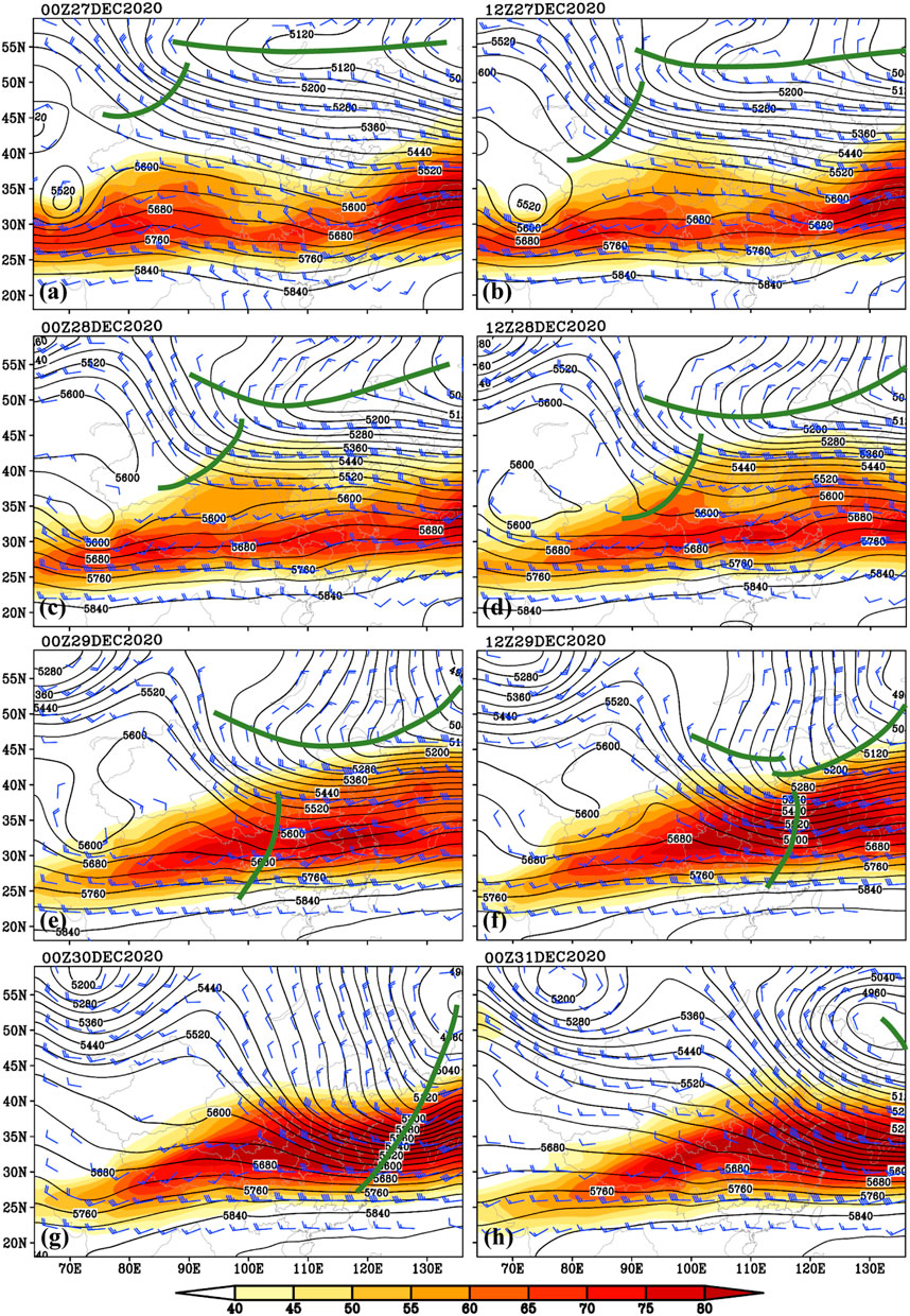
FIGURE 3. Geopotential height (black contours; gpm) and wind >10 m s⁻¹ (full bar = 10 m s⁻¹) at 500 hPa, and wind speed at 200 hPa (shading; m s⁻¹). Green lines = trough lines.

From 0000 UTC to 1200 UTC from December 29 to 31, 2020, the surface high ridge first increased (Figures 1E,F), along with its associated surface wind and cold advection (particularly in the regions east of the ridge line) before gradually weakening (Figures 1G–J), during which the ridge line broke into two sections around 0000 UTC on December 30 (Figure 1G). Correspondingly, in the middle troposphere, the transversal trough broke into two sections around 1200 UTC on December 29 (Figure 3F). The northern section then merged with T2 around 0000 UTC on December 30 (Figure 3G) and increased in intensity. After the merging, strong surface winds, intense cold advection (Figures 1I,J), and heavy snowfall (Figure 2D) mainly appeared ahead of the trough line, which was located over the sea.

After 1200 UTC on December 31, following the rapid weakening of the surface ridge, the ECW also weakened rapidly, which was reflected by a sharp weakening of the surface wind and cold advection, as well as a displacement of the 0-°C isotherm from the south to the north (not shown). Overall, the CWE lasted for ∼108 h; the maximum cold advection (around −10⁻³ K s⁻¹) and the strongest surface wind (above 20 m s⁻¹) that were associated with the CWE appeared around 0000 UTC on December 30 (Figure 1G). The heaviest CWE-associated snowfall inland occurred on December 28, 2020 (Figure 2B), which mainly covered central China. The maximum associated snowfall offshore occurred on December 29, 2020 (Figure 2C). The isotherm of 0°C reached the lowest latitude of ∼25^oN (near the north border of Guangdong Province) for this CWE at around 0000 UTC on December 31 (Figure 1I).

4 Key features and kinetic budgets of the cold wave event

4.1 Key features of the cold wave event

When the CWE began at 0000 UTC on December 27, 2020, the zonal mean (within B1) location of the 0-°C isotherm was around 38°N (Figure 4A). Within FR1, strong descending motions occurred (Figure 4B), which corresponded to a downward stretching of the zone of relatively strong wind (i.e., downward momentum transportation; Figure 4A). This contributed to the surface wind enhancement. Meanwhile, a cold front persisted at 38–50°N, in which moisture was abundant in the middle troposphere and ascending motions were dominant in the lower and middle tropospheres (Figure 4B). This provided favorable conditions for snowfall southwest of FR1 (Figure 2A). Comparison of the situations in B1 to those in B2 showed that 1)the 0-°C isotherm (thick green lines in Figures 4A, 5A) was located at a higher latitude in B2; 2) the gradients of the horizontal temperature at the lower levels (i.e., <850 hPa) were more intense for B2, implying a stronger cold front (mainly located within 40–50^oN); and 3) the downward momentum transportation within FR2 was weaker than that of FR1 (cf., Figures 4A, 5A), corresponding to a smaller surface wind.

FIGURE 4

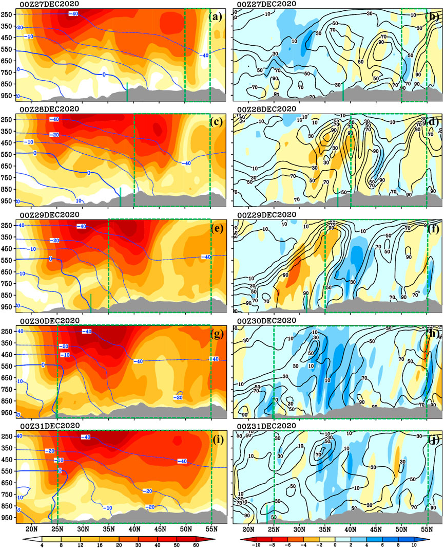
FIGURE 4. (A,C,E,G,I) Zonally (105–120^oE; B1) averaged cross-sections of wind speed (shading; m s⁻¹) and temperature (blue contours; °C). Gray shading at the bottom = terrain. Thick green lines = isotherm of 0°C. Green dashed lines = FR1. (B,D,F,H,J) The same as the left column, but for vertical velocity (shading; Pa s⁻¹) and relative humidity (black contours; %).

FIGURE 5

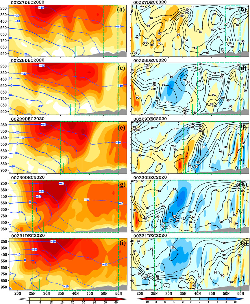
FIGURE 5. (A,C,E,G,I) Zonally (120–125^oE; the B2) averaged cross-sections of wind speed (shading; m s⁻¹) and temperature (blue contours; °C). Gray shading at the bottom = terrain. Thick green lines = isotherm of 0°C. Green dashed lines = FR2. (B,D,F,H,J) Same as the left column, but for vertical velocity (shading; Pa s⁻¹) and relative humidity (black contours; %).

From 0000 UTC to 0000 UTC from December 27 to 29, 2020, the influencing range of the CWE enlarged rapidly, with the 0-°C isotherm moving southward (Figures 4A,C,E). For B1, the surface front was enhanced, as the gradients of the horizontal temperature (around the southern boundary lines of FR1) in the lower troposphere became denser. Correspondingly, the ascending/descending motions associated with the front (shading around the southern boundary of FR1 shown in Figures 4D,F) intensified. The ascending motions were coupled with abundant moisture, which contributed to the heavy snowfall around the front (Figures 2B,C). Due to the enhancement of the strong descending motions associated with the cold front (Figure 4F), downward momentum transportation occurred in the southern section of FR1 (Figure 4E). This contributed to increased surface wind around the surface front. During the same period, similar situations to those of B1 also occurred within B2 (cf., Figures 4A–F–F4F, 5A–F–F5F); however in B2, 1) the southward movement of the 0-^oC isotherm was slower; 2) the ascending motions associated with the cold front were smaller in range but stronger in intensity in the lower troposphere (i.e., <650 hPa), which resulted in heavier snowfall (Figure 2C); 3) the downward momentum transportation was stronger around the southern boundary line of FR2 (cf., Figures 4E, 5E), and the surface wind was more intense in B2.

From 0000 UTC to 0000 UTC from December 29 to 31, 2020, for B1, the 0-°C isotherm moved southward to the southmost location during this CWE. The cold front weakened (Figures 4E,G,I) since the gradients of the horizontal temperature (around the southern boundary lines of FR1) at the lower levels became sparser. As a result, the ascending motions associated with the front weakened (Figures 4F,H,J), with the descending motions governing FR1. The surface wind around the 0-°C isotherm first increased and then decreased, with relatively stronger wind mainly located south of the 0-°C isotherm (Figures 4E,G,I). These changes indicated a weakening of the CWE inland. For B2, similar conditions appeared (cf., Figures 5E–J and Figures 4E–J): 1)the 0-^oC isotherm was located at a higher latitude; 2) the cold front was stronger and the associated descending motions were more intense; and 3) the downward momentum transportation around the southern boundary line of FR2 was stronger and the surface winds were more intense. These conditions indicated a stronger intensity of the CWE offshore than inland, implying that the land–sea distribution affected the CWE (the relative locations of the key weather systems during the CWE were also important).

4.2 Kinetic energy budget results

To understand the mechanisms governing the formation and maintenance of the strong winds associated with the CWE (the present study mainly focused on the strong winds at levels <850 hPa (LB85), which have the largest effects on human society), Eq. 4 was calculated. Before conducting detailed analyses, the comparison of LTV to TOT showed TOT/LTV values between 0.79 and 1.23 for both B1 and B2, with a mean value of ∼1.12 (not shown). This meant that the balance of Eq. 4 was overall good after neglecting the term WF; thus, the budget results could be used for further analyses.

As the gray lines in Figures 6A,B show, when the CWE began (0000 UTC 27 December 2020) at FR1 and FR2, the TOT value was positive at LB85, implying wind acceleration. At FR1, comparisons of each budget term showed that the downward transport of KE (VAD; Figure 7A) and the pressure-gradient-force’s work on the horizontal wind (WZW+WMW; Figure 8A) contributed to increased KE at LB85, while the horizontal transport (ZWA+MWA; Figure 6A) acted in an opposite manner, resulting in a net export of KE from FR1. Among all terms, WZW showed the largest positive contribution (Figure 9A) because 1) the eastward-pointing pressure gradient force (i.e., the zonal component) within FR1 was large (Figure 10A), as it linked a high-pressure ridge in the west (‘H’ in Figure 10A) and a low-pressure trough (‘L’ in Figure 10A) in the east; 2) a strong westerly wind dominated in FR1, which coupled with the large pressure gradient force aforementioned. Meanwhile, in FR2, the positive-TOT layer in the lower troposphere was thinner than that of B1 (cf., Figures 6A,B); VAD (Figure 7B), WZW, and WMW (Figure 8B) contributed to the wind enhancement at LB85, with similar intensities. ZWA+MWA was the most detrimental factor for wind intensification (Figure 6B), as it mainly caused a KE divergence within FR2.

FIGURE 6

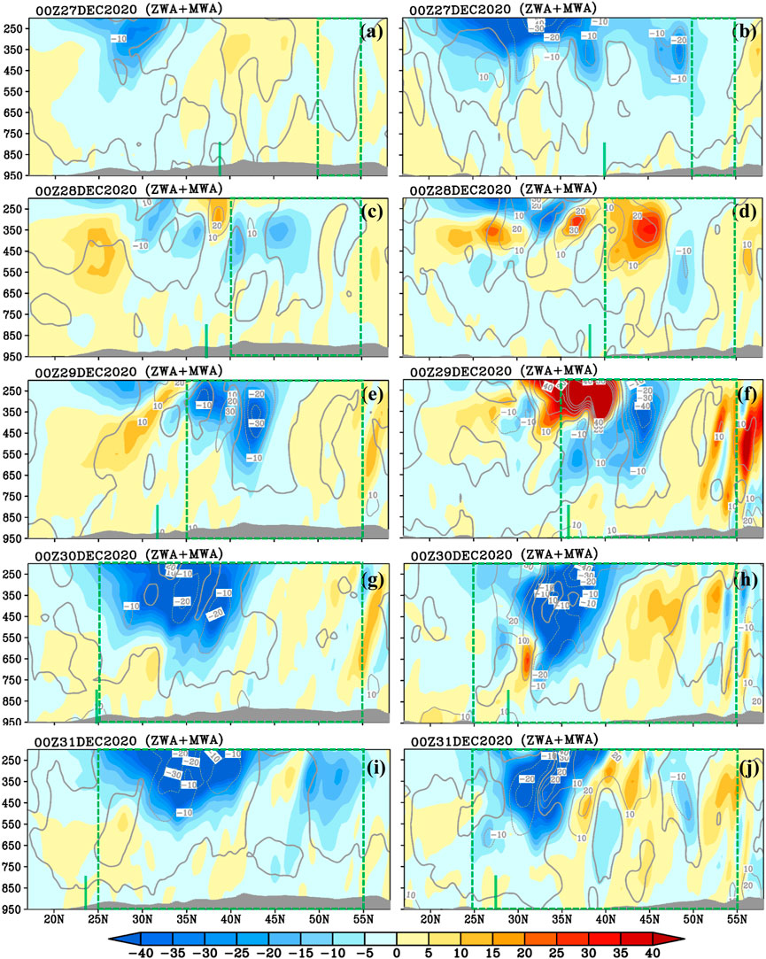
FIGURE 6. (A,C,E,G,I) Zonally (105–120^oE; the B1) averaged cross-sections of the terms ZWA (zonal wind advection) and MWA (meridional wind advection) (shading; 10⁻³ W kg⁻¹), and term TOT (gray contours; 10⁻³ W kg⁻¹). Gray shading at the bottom = terrain. Thick green lines = isotherm of 0°C. Green dashed lines = range of the FR1 of the cold wave event. (B,D,F,H,J) Same as the left column, but for the zonal average within 120–125^oE (B2).

FIGURE 7

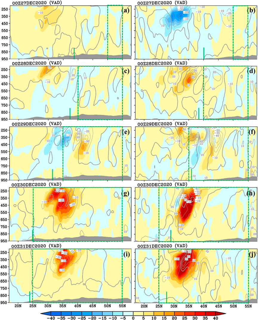
FIGURE 7. (A,C,E,G,I) Zonally (105–120^oE; B1) averaged cross-sections of the terms VAD (vertical advection) (shading; 10⁻³ W kg⁻¹), and term TOT (gray contours; 10⁻³ W kg⁻¹). Gray shading at the bottom = terrain. Thick green lines = isotherm of 0°C. Green dashed lines = range of the FR1. (B,D,F,H,J) Same as the (A,C,E,G,I), but for the zonal average within 120–125^oE (B2).

FIGURE 8

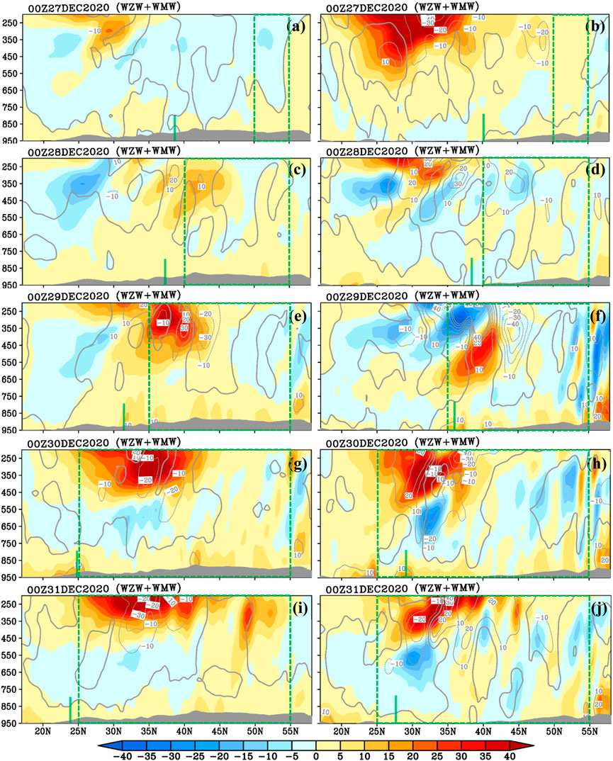
FIGURE 8. (A,C,E,G,I) Zonally (105–120^oE; the B1) averaged cross=sections of the term WZW (work of zonal wind) and WMW (work of meridional wind) (shading; 10⁻³ W kg⁻¹), and term TOT (gray contours; 10⁻³ W kg⁻¹). Gray shading at the bottom = terrain. Thick green lines = isotherm of 0°C. Green dashed lines = range of FR1. (B,D,F,H,J) Same as the left column, but for the zonal average within 120–125^oE (B2).

FIGURE 9

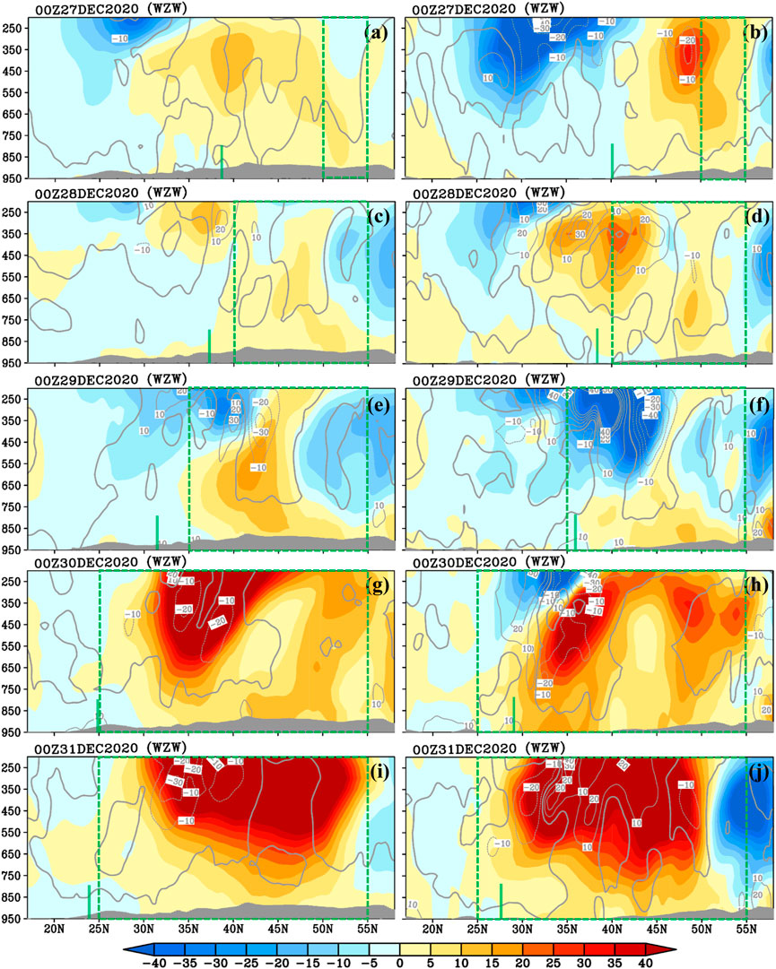
FIGURE 9. (A,C,E,G,I) Zonally (105–120^oE; B1) averaged cross=sections of the terms WZW (work of zonal wind) (shading; 10⁻³ W kg⁻¹), and term TOT (gray contours; 10⁻³ W kg⁻¹). Gray shading at the bottom = terrain. Thick green lines = isotherm of 0°C. Green dashed lines = range of the FR1 of the cold wave event. (B,D,F,H,J) Same as (A,C,E,G,I), but for the zonal average within 120–125^oE (B2).

FIGURE 10

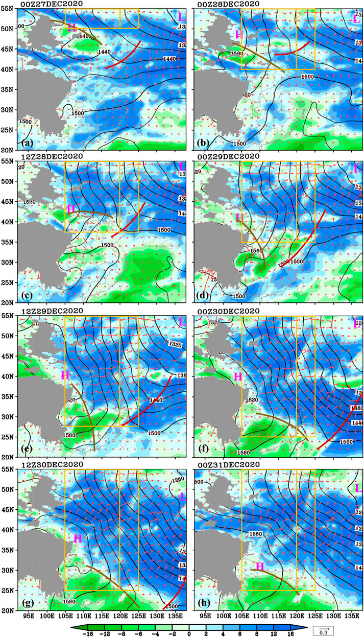
FIGURE 10. Zonal wind (shading; m s⁻¹), geopotential height (black contours; gpm), and −$\nabla \Phi$ (red vectors; m s⁻²) at 850 hPa. Gray shading = terrain above 1,500 m. ‘H’ high-pressure system. ‘L’ = low-pressure system. Thick red lines = trough lines. Thick brown lines = ridge lines. Yellow boxes = FR1/FR2 of the cold wave event.

From 0000 UTC 27 to 0000 UTC 29 December 2020, both FR1 and FR2 mainly showed a positive TOT at LB85 (gray contours in Figures 6A–F), implying that conditions were favorable for the enhancement or maintenance of the KE associated with the CWE during this period. As the downward momentum transportation appeared within FR1 and FR2, the VAD contributed to KE enhancement in both (Figures 7A–F), more strongly in FR1 than in FR2. Corresponding to the enhancement and southward extension of the high- and low-pressure systems in the lower troposphere (‘H’ and ‘L’ in Figures 10A–D), the eastward-pointing pressure gradient force increased and maintained a strong intensity. According to Eq. 1, the strong pressure gradient force contributed to the intensification of the westerly wind. Therefore, as aforementioned, the eastward-pointing pressure gradient force did positive work on the westerly wind (Figures 10A–D), which resulted in a strong WZW at LB85 of both FRs (Figures 9A–F). This acted as the dominant factor for the KE increase. The comparison of Figures 8A–F to Figures 9A–F showed that the WMW mainly weakened the KE at LB85 of both FRs. The ZWA+MWA was mainly negative at LB85 of FR1 (Figures 6A,C,E), whereas, for LB85 of FR2, it changed gradually from negative to positive (Figures 6B,D,F). Thus, in FR2, the horizontal transport of the KE changed from divergence (decelerated wind) to convergence (accelerated wind). The change in sign in ZWA+MWA within FR2 was mainly due to the eastward transport of KE by the westerly wind from FR1 to FR2 (not shown), which transported the KE within FR1 to FR2.

From 0000 UTC 29 to 0000 UTC 30 December 2020, at the LB85, the TOT value remained positive in both FRs (gray lines in Figures 6E–H), with strong TOT centers (≥10 ×10⁻³ W kg⁻¹) mainly located around the southern boundary lines of FR1 and FR2 (Figures 6E–H), particularly in the regions south of the boundary lines. This explained the strong lower-level winds in these regions (Figures 4G, 5G). Comparisons of the overall features of LB85 of FR1 to those of FR2 showed that 1) the TOT was stronger for FR2, which corresponded to a stronger low-level wind; 2) the horizontal transport of KE (i.e., ZWA+MWA) mainly reduced the KE within FR1 (Figures 6E,G), whereas for FR2, it first contributed to the KE increase and then mainly showed a neutral effect (Figures 6F,H); 3) the downward KE transportation (i.e., VAD) increased with time and acted as a favorable factor to enhance the KE within both FRs (Figures 7E–H); 4) the work force of the pressure gradient (i.e., Figures 8E–H) was the most favorable factor for KE enhancement in both FRs. Comparison of Figures 8E–H to Figures 9E–H showed that, among all terms, the WZW made the dominant contribution to the positive TOT for both FRs. However, around the southern boundary lines of the FRs, the WZW mainly showed a negative contribution (Figures 9E–H) because the southern boundary lines of the FRs were located around the southern periphery of the high-pressure system in the lower troposphere (Figures 10D–F), where the easterly wind was strong. The eastward-pointing pressure gradient force demonstrated negative work on the easterly wind. As a result, for the strong TOT centers around the southern boundary lines of the FRs, the WMW contributed the most (Figures 8E–H). This was different from the situations of the overall features of FR1 and FR2 discussed previously.

From 0000 UTC 30 to 0000 UTC 31 December 2020, at LB85 of both FRs, the positive TOT weakened notably (gray lines in Figures 6G–J), implying that the conditions becoming unfavorable for maintaining the strong winds associated with the CWE. During this period, the horizontal transport of the KE was mainly detrimental to maintaining the KE at the LB85 of the FRs (Figures 6I,J). The vertical KE transportation still contributed to sustaining the KE and kept a relatively strong intensity (Figures 7I,J). The work force of the pressure gradient on the horizontal wind decreased in intensity (Figures 8I,J), as the high-pressure system in the lower troposphere weakened significantly and its associated westerly wind decelerated (Figures 10F–H). However, WZW+WMW still showed a favorable effect for sustaining the lower-level KE (Figures 8I,J), with WZW stronger than WMW (Figures 9I,J).

5 Effects of the cold wave event on wind power generation

5.1 Features of the wind power density at 100 m

As Eq. 5 shows, the WPD was determined by both air density and wind speed. When the CWE occurred, the wind accelerated quickly (i.e., the dynamic contribution). Meanwhile, the air temperature decreased rapidly, which increased the air density (i.e., the thermodynamic contribution). Thus, the WPD was enhanced during the CWE (in most cases, the dynamic contribution was much larger than the thermodynamic contribution). Since most wind turbines were around 100 m in height in this study, we evaluated the WPD at 100 m during the CWE.

As Figure 11A shows, when the CWE began (0000 UTC 27 December 2020), relatively strong winds (at 100 m) mainly appeared within KR1. The WPD within both FRs was mainly <250 W m⁻², with some regions around 120°E even at <20 W m⁻². From 0000 UTC 27 to 0000 UTC 28 December 2020, the wind within FR1 enhanced more rapidly than that of FR2; therefore, the WPD of the former also intensified more quickly (Figure 11B). From 0000 UTC 28 to 1200 UTC 28 December 2020, the influencing regions of the CWE were mainly located inland (Figure 11C). The WPD within both FRs increased, with the southern section of FR2 (which was mainly located over the Bohai Sea) showing the largest WPD (2000–2500 W m⁻²), mainly because the friction force offshore was much smaller than that inland. From 0000 UTC 29 to 1200 UTC 30 December 2020, as the high-pressure system at the surface enlarged southeastward, the influencing regions of the CWE extended to the sea (Figures 11D–G). During this period, the WPD within the southern section of FR2, which was mainly located offshore, showed the strongest intensity (up to 5000 W m⁻² or more), as deceleration due to friction was small there. In FR1, a relatively strong WPD (∼1000 W m⁻²) was mainly situated in the northern section, where the eastward-pointing pressure gradient force was strong (Figures 10D–G) and did positive work on the strong westerly wind. In contrast, in the southern section of FR1, the WPD was relatively weak. From 1200 UTC to 0000 UTC from December 30 to 31, 2020, as the high-pressure system weakened rapidly (Figure 11H), the WPD within both FRs decreased. This was consistent with the weakening of the CWE. In this period, a relatively strong WPD mainly appeared within the northern section of FR1 and the southern section of FR2, where the 100-m wind was >10 m s⁻¹.

FIGURE 11

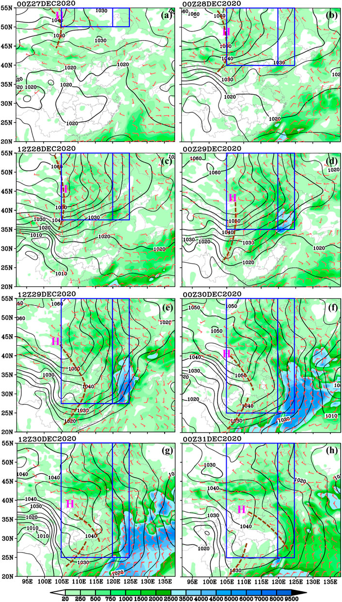
FIGURE 11. Wind power density (shading; W m⁻²) and wind speed >4 m s⁻¹ (full bar = 4 m s⁻¹) at 100 m above the ground level. ‘H’ = high-pressure system. Brown dashed lines = ridge lines. Blue boxes = FR1 and FR2 of the cold wave event.

Overall, the variation in WPD was consistent with the variation in the CWE. Stronger WPD tended to appear within the northern section of FR1, the southern section of FR2, and the regions south of the boundary line of FR1. All these regions featured dense isobars, implying strong winds (according to the theory of geostrophic wind; Holton, 2004). Comparison of WPD inland and offshore showed a generally much larger WPD offshore. This might be partly due to the much smaller friction over the sea than those on land. During the CWE, extremely strong WPD for wind speeds >25 m s⁻¹ rarely occurred, indicating that the high-wind-velocity cut-out percentage of the wind turbines was negligible; therefore, most of the strong winds associated with the CWE could be used to generate wind power.

5.2 Comparisons to the mean state

To evaluate the effects of the CWE on the WPD, we compared the temporal mean of the WPD during the winters of 2016–2020 (defined as the mean state) to the temporal mean of the WPD during the CWE discussed in the present study. Based on the influencing area and movement of the CWE, six comparison regions were defined, as shown in the gray dashed lines in Figure 12 (located within B1 and B2, which were affected by the strong winds associated with the CWE). As shown in Figure 12A, in the mean state, region III showed the largest percentage of zero wind power generation due to low wind velocity (39.5%), followed by region V (35.9%). In contrast, within regions I, II, IV, and VI, the percentages of zero wind power generation were around 10%. Due to the wind enhancement of the CWE, within all six comparison regions, the percentages of zero wind power generation all decreased (from 1.4% to 13.7%), particularly in regions III and V (Figures 12B,C). No obvious changes in high-wind-velocity cut-out percentages were observed within the six comparison regions (Figure 12D) as wind speeds >25 m s⁻¹ were unusual in this CWE. As discussed previously, the CWE notably reduced the percentage of zero wind power generation due to low wind velocity, while maintaining the high-wind-velocity cut-out percentage. This improved the availability of the wind to generate power.

FIGURE 12

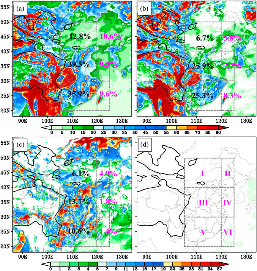
FIGURE 12. (A) Percentage of zero wind power generation due to low wind velocity (calculated using the wind speed at 100 m above the ground level) during the winters of 2016–2020 (shading; %). Thick black line = terrain at 1,500 m. Gray dashed boxes = six comparison areas (I-VI; Figure 12D). Numbers = region-averaged percentages, respectively. (B) Same as that of (A), but for the period during the cold wave event discussed in this study. (C) Results of the calculations of (A) minus (B). (D) Same as (C) but for the high-wind-velocity cut-out percentage (shading; %).

As Figure 13 shows, for all six comparison regions, the WPD was notably enhanced during the CWE. The largest increasing ratio appeared within region IV (184.1%), and the increasing ratios within regions III, V, and VI were all >100%. The smallest increasing ratio was observed within region II (28.2%), followed by region I (46.1%). As discussed previously, the CWE could have contributed to wind power generation by the WPD.

FIGURE 13

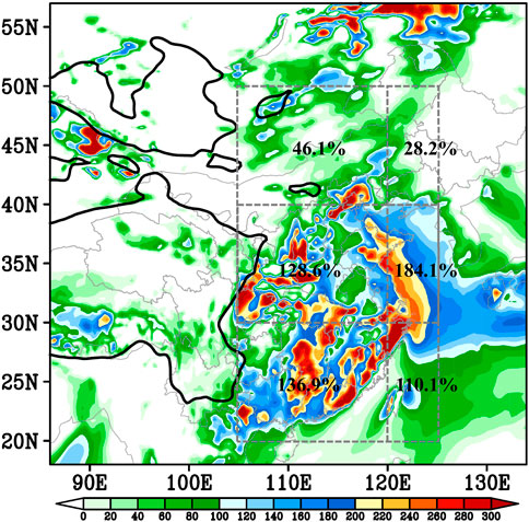
FIGURE 13. Increasing ratio (shading; %) of the temporal average of the wind power density during the cold wave event discussed in this study relative to that during the winters of 2016–2020. Thick black line = terrain at 1,500 m. Gray dashed boxes = six comparison areas (I–VI; Figure 12D). Numbers = region-averaged increasing ratios, respectively.

Overall, the effect of the CWE on the percentage of zero wind power generation due to low wind velocity was closely related to the land–sea distribution: the CWE caused a more obvious reduction in the percentage of zero wind power generation inland compared to that offshore (regions I–III and V versus regions IV and VI are in Figure 12C), mainly due to stronger offshore winds compared to those inland. In contrast, the effects of the CWE on the WPD were closely related to the region latitudes: the middle latitudes in this event showed the largest increasing ratio, whereas the higher latitudes showed the smallest increasing ratio (comparisons among regions I–II, II–IV, and V–VI are shown in Figure 13), mainly because the high-pressure system at the surface produced strong 100-m winds during this event, with the largest/smallest intensities (represented by the temporal mean isobar density during the CWE) in the middle/higher latitudes (data not shown).

6 Conclusion and discussion

CWEs are among the most important types of disastrous weather during the cold season, often causing major economic losses and serious casualties. Under global warming, the frequency and intensity of CWEs have tended to increase; thus, their threats to the environment and human society are enhanced. Therefore, studies on CWE have attracted increased attention. In late December 2020, an intense CWE occurred in China, lasted for ∼108 h, and broke a series of historical records. To fill the knowledge gaps discussed in the introduction, we applied a KE budget analysis to the CWE-associated strong winds and conducted quantitative comparisons of the key features of the wind energy during the CWE compared to those in the mean state.

The results of the synoptic analyses indicated that the CWE occurred under favorable background conditions, which were characterized by a southward-moving transversal trough and a southeastward-moving shortwave trough in the middle troposphere (the northerly wind in the central region of the transversal trough and the northwesterly wind behind the shortwave trough steered intensely cold air from higher to lower latitudes). The surface high ridge that formed around Lake Baikal (and developed southeastward) and the cold front around the southern periphery of the ridge were key factors governing the CWE evolution. Influenced by the land–sea distribution, the CWE showed notably different features inland and offshore: the 0-°C isotherm was located at a lower latitude inland, the southward movement of the 0-°C isotherm was slower, the cold front and snowfall were stronger, and the downward momentum transportation and maximum surface wind were more intense offshore.

The KE budget analysis indicated that the positive effect on the horizontal wind by the pressure-gradient-force (mainly due to the eastward-pointing pressure gradient force that linked a lower tropospheric high-pressure ridge inland and a low-pressure trough offshore), and the downward transport of KE from higher levels to near-surface levels (mainly due to the descending motions behind the cold front) acted as the dominant and second dominant factors for the enhancement and sustainment of CWE-associated strong winds. In contrast, the horizontal transport mainly resulted in a net export of KE, which weakened the strong winds.

Analyses of the WPD features affected by the CWE showed enhancement of different magnitudes within different regions (the increasing ratios ranged from 28.2% to 184.1%, with a mean value of 105.7%), implying that the CWE could contribute to wind power generation by increasing the WPD. In addition, the CWE reduced the percentage of zero wind power generation (due to low wind velocity) by 1.4%–13.7%, while the high-wind-velocity cut-out percentage was almost unchanged. This could improve the availability of wind for generating electricity. Overall, the WPD variation was consistent with the variation in the CWE. The effects of the CWE on increasing WPD were closely related to the regions’ latitudes, with middle latitudes showing the largest increase in ratio. Moreover, the effects of the CWE on reducing the percentage of zero wind power generation (due to low wind velocity) were closely related to those of the land–sea distribution, with more obvious reductions in inland regions.

However, as we only investigated one CWE, the quantitative results of the comparisons between the CWE and the mean state might have limitations in representing the real situation. As the CWE could increase the WPD and improve the availability of the wind for generating electricity (for some extreme CWEs with minimum temperatures <−30°C, the wind turbines should be shut down for safety), we suggest the need for more studies on CWEs to provide a more comprehensive understanding of CWE-associated strong winds and useful reference for wind power generation. Fu et al., 2022, Liang et al., 2014.

Data availability statement

The original contributions presented in the study are included in the article/Supplementary Material. Further inquiries can be directed to the corresponding authors.

Author contributions

HM, SJ, and SF designed the research. HM, GL, CZ, FW, and SJ performed the research. All authors wrote the manuscript, contributed to the article, and approved the submitted version.

Funding

This research was supported by the National Natural Science Foundation of China (Grant Nos 42075002 and U2142202).

Conflict of interest

The author HM was employed by Beijing Goldwind Smart Energy Technology Co., Ltd. The author GL was employed by State Grid Xinjiang Electric Power Co., Ltd. The author CZ was employed by China Resources Power Technology Research Institute Co., Ltd.

The remaining authors declare that the research was conducted in the absence of any commercial or financial relationships that could be construed as a potential conflict of interest.

Publisher’s note

All claims expressed in this article are solely those of the authors and do not necessarily represent those of their affiliated organizations, or those of the publisher, the editors, and the reviewers. Any product that may be evaluated in this article, or claim that may be made by its manufacturer, is not guaranteed or endorsed by the publisher.

References

Aboobacker, V. M., Shanas, P. R., Veerasingam, S., Al-Ansari, E. M. A. S., Sadooni, F. N., and Vethamony, P. (2021). Long-term assessment of onshore and offshore wind energy potentials of Qatar. Energies 14, 1178. doi:10.3390/en14041178

CrossRef Full Text | Google Scholar

Bueh, C., Peng, J. B., Lin, D. W., and Chen, B. M. (2022). On the two successive supercold waves straddling the end of 2020 and the beginning of 2021. Adv. Atmos. Sci. 39 (4), 591–608. doi:10.1007/s00376-021-1107-x

CrossRef Full Text | Google Scholar

Cattiaux, J., Vautard, R., Cassou, C., Yiou, P., Masson-Delmotte, V., and Codron, F. (2010). Winter 2010 in europe: A cold extreme in a warming climate. Geophys. Res. Lett. 37704. doi:10.1029/2010gl044613

CrossRef Full Text | Google Scholar

Cherp, A., Vinichenko, V., Tosun, J., Gordon, J. A., and Jewell, J. (2021). National growth dynamics of wind and solar power compared to the growth required for global climate targets. Nat. Energy 6, 742–754. doi:10.1038/s41560-021-00863-0

CrossRef Full Text | Google Scholar

Cohen, J., Screen, J., Furtado, J., Barlow, M., Whittleston, D., Coumou, D., et al. (2014). Recent Arctic amplification and extreme mid-latitude weather. Nat. Geosci. 7, 627–637. doi:10.1038/ngeo2234

CrossRef Full Text | Google Scholar

IPCC (2012). Summary for policymakers. Managing the risks of extreme events and disasters to advance climate change adaptation. Editors C. B. Field, V. Barros, T. F. Stocker, D. Qin, D. J. Dokken, K. L. Ebiet al. (Cambridge, United Kingdom: Cambridge University Press), 3–21.

Google Scholar

Fu, S.-M., Yu, F., Wang, D.-H., and Xia, R.-D. (2013). A comparison of two kinds of eastward-moving mesoscale vortices during the mei-yu period of 2010. Sci. China Earth Sci. 56, 282–300. doi:10.1007/s11430-012-4420-5

CrossRef Full Text | Google Scholar

Fu, S.-M., Zhang, J.-P., Sun, J.-H., and Zhao, T.-B. (2016). Composite analysis of long-lived mesoscale vortices over the middle reaches of the Yangtze River valley: Octant features and evolution mechanisms. J. Clim. 29, 761–781. doi:10.1175/jcli-d-15-0175.1

CrossRef Full Text | Google Scholar

Fu, S.-M., Zhang, Y.-C., Wang, H.-J., Tang, H., Li, W.-L., and Sun, J.-H. (2022). On the evolution of a long-lived mesoscale convective vortex that acted as a crucial condition for the extremely strong hourly precipitation in Zhengzhou. JGR. Atmos. 127, e2021JD036233. doi:10.1029/2021jd036233

CrossRef Full Text | Google Scholar

Fu, S. M., Zhao, S. X., Sun, J. H., and Qi, L. L. (2012). Energy budget of a cold surge process during the winter monsoon period of 2004. Clim. Environ. Res. (in Chinese) 17 (5), 549–562.

Google Scholar

Geert, J., Eli, M., Gabriel, A., Hylke, V., Robert, V., and Friederike, O. (2019). Cold waves are getting milder in the northern midlatitudes. Environ. Res. Lett. 14, 114004. doi:10.1088/1748-9326/ab4867

CrossRef Full Text | Google Scholar

Gualtieri, G. (2021). Reliability of ERA5 reanalysis data for wind resource assessment: A comparison against tall towers. Energies 14, 4169. doi:10.3390/en14144169

CrossRef Full Text | Google Scholar

Hersbach, H., Bell, B., Berrisford, P., Hirahara, S., Horanyi, A., Munoz Sabater, J., et al. (2020). The ERA5 global reanalysis. Q. J. R. Meteorol. Soc. 146, 1999–2049. doi:10.1002/qj.3803

CrossRef Full Text | Google Scholar

Holton, J. R. (2004). An introduction to dynamic meteorology. San Diego: Academic Press, 552pp.

Google Scholar

Huffman, G. J., Stocker, E. F., Bolvin, D. T., Nelkin, E. J., and Tan, Jackson (2019). “GPM IMERG final precipitation L3 1 day 0.1 degree x 0.1 degree V06,” in Goddard earth Sciences data and information services center. Editors Andrey Savtchenko, and M. D. Greenbelt, Vol. 1. https://www.re3data.org/repository/r3d100000036. doi:10.25504/FAIRsharing.7388wt

CrossRef Full Text | Google Scholar

Jiang, Dachuan, Jiang, D., Xiao, Weihua, Xiao, W., Wang, Jianhua, Wang, J., et al. (2018). Evaluation of the effects of one cold wave on heating energy consumption in different regions of northern China. Energy 142, 331–338. doi:10.1016/j.energy.2017.09.150

CrossRef Full Text | Google Scholar

Liang, S. J., Ding, Y. H., Zhao, N., and Sun, Y. (2014). Analysis of the interdecadal changes of the wintertime surface air temperature over mainland China and regional atmospheric circulation characteristics during 1960–2013 (in Chinese). Chinese of Journal Atmospheric Science 38 (5), 974–992.

Google Scholar

Ma, S. M., and Zhu, C. W. (2020). Opposing trends of winter cold extremes over eastern Eurasia and North America under recent Arctic warming. Adv. Atmos. Sci. 37 (12), 1417–1434. doi:10.1007/s00376-020-0070-2

CrossRef Full Text | Google Scholar

Mu, M., Luo, D. H., and Zheng, F. (2022). Preface to the special issue on extreme cold events from east asia to north America in winter 2020/21. Adv. Atmos. Sci. 39 (4), 543–545. doi:10.1007/s00376-021-1004-3

CrossRef Full Text | Google Scholar

Pryor, S. C., and Barthelmie, R. J. (2021). A global assessment of extreme wind speeds for wind energy applications. Nat. Energy 6, 268–276. doi:10.1038/s41560-020-00773-7

CrossRef Full Text | Google Scholar

Qian, C., Zhang, X., and Li, Z. (2019). Linear trends in temperature extremes in China, with an emphasis on non-Gaussian and serially dependent characteristics. Clim. Dyn. 53, 533–550. doi:10.1007/s00382-018-4600-x

CrossRef Full Text | Google Scholar

Qian, W. H., and Zhang, W. W. (2007). Changes in cold wave events and warm winter in China during the last 46 years. Chinese Journal of Atmospheric Sciences 31, 1266–1278.

Google Scholar

Wen, Y., Kamranzad, B., and Lin, P. Z. (2021). Assessment of long-term offshore wind energy potential in the south and southeast coasts of China based on a 55-year dataset. Energy 224, 120225. doi:10.1016/j.energy.2021.120225

CrossRef Full Text | Google Scholar

Yuan, J. (2016). Wind energy in China: Estimating the potential. Nat. Energy 1, 16095. doi:10.1038/nenergy.2016.95

CrossRef Full Text | Google Scholar

Zhang, L., Xie, Z., Deng, Y., and Huang, W. (2021). Structure and large-scale organization of extreme cold wave events over the Chinese mainland during the boreal cold season. JGR. Atmospheres 126, e2021JD035005. doi:10.1029/2021JD035005

CrossRef Full Text | Google Scholar