Adaptive variable-grid least-squares reverse-time migration

Variable-grid methods have the potential to save computing costs and memory requirements in forward modeling and least-squares reverse-time migration (LSRTM). However, due to the inherent difficulty of automatic grid discretization, conventional variable-grid methods have not been widely used in industrial production. We propose a variable-grid LSRTM (VG-LSRTM) method based on an adaptive sampling strategy to improve computing efficiency and reduce memory requirements. Based on the mapping relation of two coordinate systems, we derive variable-grid acoustic wave equation and its corresponding Born forward modeling equation. On this basis, we develop a complete VG-LSRTM framework. Numerical experiments on a layered model validate the feasibility of the proposed VG-LSRTM algorithm. LSRTM tests on a modified Marmousi model demonstrate that our method can save computational costs and memory requirements with little accuracy loss.

Introduction

Migration technologies play an increasingly significant role in seismic data processing (Yilmaz, 2001). Reverse time migration (RTM) (Baysal et al., 1983; Whitmore, 1983), which uses two-way wave equations for wavefield propagation, is regarded as the most effective method for imaging steep dip and complex structures. Compared with one-way wave-equation migration (Claerbout, 1971; Xie and Wu, 2005) and ray-based migration methods (Schneider, 1978; Hill, 1990), RTM has no dip limitation and can correctly image prism and overturned waves. RTM has been widely studied and developed by many scholars because of its advantage in providing high-accuracy subsurface images (Sun and McMechan, 2001; Rocha et al., 2016; Du et al., 2017). However, RTM images usually suffer from artifacts (Zhang and Sun, 2009), incomplete illumination (Buur and Kühnel, 2008) and low-frequency noise (Díaz and Sava, 2016) because conventional RTM algorithm uses the adjoint of the linearized wave equation rather than its inverse (Nemeth et al., 1999).

Inverse theory-based least-squares migration (LSM) (Lailly and Bednar, 1983) aims to obtain images with fewer artifacts and acquisition marks by approximating the exact inverse of the wave equation modeling operator (Lambaré et al., 1992; Kühl and Sacchi, 2003; Hu et al., 2016). Using the RTM operator to perform migration procedure under the framework of LSM leads to least-squares reverse-time migration (LSRTM) (Dai et al., 2012; Dong et al., 2012). The data-domain LSRTM method seeks to iteratively update the subsurface reflectivity by minimizing the residual between the simulated data and observed data (Dai and Schuster, 2013; Zhang et al., 2015; Wang et al., 2017). It has been extended to elastic (Feng and Schuster, 2017; Ren et al., 2017; Gu et al., 2018), viscoacoustic (Dutta and Schuster, 2014; Sun et al., 2016; Chen et al., 2017; Yang and Zhu, 2019) and anisotropic cases (Qu et al., 2017; Yang et al., 2019; Mu et al., 2020) due to its superiority in balancing amplitude, suppressing artifacts, and improving image resolution. However, limited by large computing costs (Dai and Schuster, 2013), the sensitivity to migration velocity (Tan and Huang, 2014; Li et al., 2017), and the mismatch of amplitudes (Zhang et al., 2015), conventional LSRTM is not extensively used in large-scale field data processing.

Many researchers have done valuable work to accelerate LSRTM. Dai et al. (2012) used multi-source strategy to improve the computing efficiency of LSRTM. After that, Dai and Schuster (2013), Li et al. (2018), Liu and Liu (2018), Zhao and Sen (2019), and Li et al. (2020) successively applied plane-wave theory and encoding technologies to LSRTM to reduce the computational costs. However, the crosstalk noise often occurs in LSRTM images when using the multi-source encoding algorithms, which seriously degrades the inversion quality. Speeding up the convergence rate of LSRTM is another way to save production costs. Duprat and Baina (2016) introduced a preconditioning factor into LSRTM and achieved fast convergence results. Rocha et al. (2018) developed an energy-based LSRTM algorithm to speed up the convergence of LSRTM. Thanks to the development of high-performance computer, the GPU/CPU parallel LSRTM algorithm has been developed to improve the efficiency (Xue and Liu, 2017; Zhang et al., 2018). In recent reports, some deep-learning frameworks have been used to alleviate the computing burden (Vamaraju et al., 2021) and reduce the number of iterations (Kristian and Mauricio, 2022) of conventional LSRTM.

Another promising application to speed up LSRTM is using the model-driven variable-grid methods. The use of irregular spatial grid interval can be traced back to Moczo’s (1989) finite-difference modeling for SH-waves. Jastram and Behle (1992) proposed variable-grid spacing algorithm in depth domain and applied it to solve two-dimensional acoustic wave equation. Then, Jastram and Tessmer (1994) developed this method into elastic cases. Falk et al. (1996) used varying grid spacing to simulate the tube wavefield successfully. The variable-grid algorithms mentioned above usually use different finite-difference coefficients in the transition region between coarse and fine grids. Wang and Schuster (1996) proposed an interpolation-based variable-grid method for elastic and acoustic wave equation modeling. Wang (2001) further developed interpolation strategy into viscoelastic wave simulation. The variable-grid strategy has been successfully applied to waveform inversion and RTM. Ha and Shin (2012) developed an axis transformation method to speed up Laplace-domain full-waveform inversion (FWI). Li et al. (2014) proposed an efficient dual-variable algorithm and applied it to RTM. Sun et al. (2017) introduced the variable-grid technique into cross-well seismic data imaging. Wang et al. (2017) developed an adaptive FWI algorithm based on the variable-grid strategy to reduce the computational costs.

Since wavefield simulation and RTM are the basic units of LSRTM, these variable-grid methods mentioned above have the potential to accelerate LSRTM. However, there are many difficulties in applying them to LSRTM. First, conventional variable-grid algorithms always sample a specified area, the edge of which generates strong spurious reflections because the grid size in this area is much smaller than that in other areas. Such spurious reflections are hard to eliminate in seismic wave propagation, and is likely to reduce the quality of LSRTM images. Second, it is necessary to change the finite-difference scheme or coefficients of the transition regions between spatial grids of different sizes to achieve successful wavefield extrapolation, which poses challenges of accuracy and stability for the implementation of variable-grid LSRTM (VG-LSRTM). Finally, due to the difficulty inherent in automatically gridding complex velocity model, conventional variable-grid methods are not so practical and they are hardly applied to LSRTM. The pseudo-time domain method (Alkhalifah, 2003; Ma and Alkhalifah, 2013) provides a global grid discretization strategy to overcome these problems, which can be considered as a special variable-grid method. Li et al. (2017) developed a cross-correlation LSRTM algorithm in pseudo-time domain (PT-LSRTM) to improve the computing efficiency and reduce the sensitivity of velocity errors to imaging results. However, the demigration operator in pseudo-time domain is more complicated than that in depth domain. Therefore, PT-LSRTM cannot significantly reduce the computational costs.

To improve the computing efficiency of LSRTM without precision loss, we propose an adaptive VG-LSRTM algorithm based on a global sampling strategy in this paper. Our variable-grid approach is efficient and convenient, which does not require changing the finite-difference scheme and its coefficients, adding the transition region between grids of different sizes, and manually gridding the velocity model. We first derive a variable-grid first-order acoustic wave equation and the corresponding demigration equation based on a mapping relationship. Then, two numerical tests on synthetic data demonstrate the advantages of our method. After that, we discuss the possible risks of the proposed method in terms of stability and accuracy. Finally, we summarize the paper in the conclusion section.

Methodology

Adaptive sampling method and variable-grid acoustic wave equation

The 2D first-order velocity-stress acoustic wave equation in an inhomogeneous isotropic media is written as:

$\begin{array}{l}\rho \frac{\partial u}{\partial t}=\frac{\partial p}{\partial x}\\ \rho \frac{\partial w}{\partial t}=\frac{\partial p}{\partial z}\\ \frac{1}{\rho v^2}\frac{\partial p}{\partial t}=\frac{\partial u}{\partial x}+\frac{\partial w}{\partial z}+S\left(t\right)\end{array}(1)$

where $u$ and $w$ are the particle velocity, $p$ is acoustic pressure field, $\rho$ is medium density, $v$ is acoustic velocity, and $S\left(t\right)$ is the source term.

Eq. 1 has been widely used in forward modeling and LSRTM (Virieux, 1986; Li et al., 2017). It is easier to obtain better results by using finer spatial grid than coarser one when applying the finite-difference technique to solve Eq. 1. However, for those high-velocity zones, the use of fine grid leads to a waste of computing resources. In this section, we introduce an adaptive sampling method to solve the above problem based on the assumption that the formation velocity varies with depth and properties of the underground media.

Given an initial velocity model whose number of grid points and spatial grid spacing are already known. We use Eq. 2 to calculate its optimal vertical grid spacing along the depth direction:

$dz\left(z\right)=\frac{v_{\min }\left(z\right)}{f_{d}k}(2)$

where $dz\left(z\right)$ denotes the optimal vertical grid spacing in depth $z$, $v_{\min }\left(z\right)$ is the minimum velocity of each layer along z-axis, $k$ denotes the number of vertical grid points per wavelength, and $f_d$ denotes the maximum frequency of the source. Obviously, $dz\left(z\right)$ decreases as $k$ and $f_d$ increase. To ensure that the grid dispersion never occur, $k$ is set to ten in this paper.

In order to keep the total depth of the initial model constant, we resample it using an adaptive sampling method. The process is illustrated in Figure 1. The horizontal axis in Figure 1 denotes depth of the initial model and the black dashed line in Figure 1 denotes the optimal vertical grid spacing. First, we take a small trial step from the surface of the model and gradually increase it to obtain the first grid point $z_1$, where $z_1=dz\left(z_1\right)$. Then we use the same way to get the next grid point $z_2$, where $z_2-z_1=dz\left(z_2\right)$. Next, we repeat this process to the maximum depth of the model and get all of the grid points. In high-velocity zone, the grid interval is larger than that in low-velocity zone, and the grid points are sparser, which makes grid discretization more reasonable compared with regular-grid implementation. Now we obtain a new model, which has variable vertical grid interval. We keep the horizontal grid interval constant because the formation velocity varies mainly along the depth direction and our adaptive sampling method is not applicable to areas where the medium velocity changes slowly.

FIGURE 1

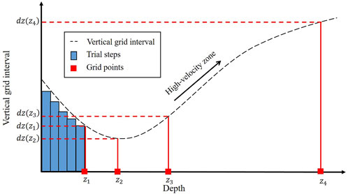
FIGURE 1. Principle of the adaptive sampling.

The initial model is located in Cartesian coordinate system $M\left(x,z\right)$ while the new model is located in a new rectangular coordinate system $N\left(\xi ,\eta \right)$. There is a mapping relationship between the coordinate variables of the two coordinate systems. We use Eq. 3 to express this relation:

$\begin{array}{l}\xi =x\\ \frac{\partial \eta }{\partial z}=\phi \left(z\right)\end{array}(3)$

where the $\xi$ and $\eta$ are the coordinate variables in $N\left(\xi ,\eta \right)$, $x$ and $z$ are the coordinate variables in $M\left(x,z\right)$, and $\phi \left(z\right)$ denotes the mapping relationship. It is important to note that the based on the adaptive sampling shown in Figure 1, $\eta$ does not depend on $x$.

Thus, Eq. 1 can be rewritten as:

$\begin{array}{l}\rho \frac{\partial u}{\partial t}=\frac{\partial p}{\partial \xi }=\frac{\partial p}{\partial x}\\ \rho \frac{\partial w}{\partial t}=\frac{\partial p}{\partial \eta }=\frac{\partial p}{\partial z}\frac{\partial z}{\partial \eta }=\frac{\partial p}{\partial z}\frac{1}{\phi \left(z\right)}\\ \frac{1}{\rho v^2}\frac{\partial p}{\partial t}=\frac{\partial u}{\partial \xi }+\frac{\partial w}{\partial \eta }+S\left(t\right)\\ =\frac{\partial u}{\partial x}+\frac{\partial w}{\partial z}\frac{\partial z}{\partial \eta }+S\left(t\right)\\ =\frac{\partial u}{\partial x}+\frac{\partial w}{\partial z}\frac{1}{\phi \left(z\right)}+S\left(t\right)\end{array}(4)$

Eq. 4 is the variable-grid acoustic wave equation, which can be solved in $M\left(x,z\right)$ by means of the mapping relation. Its computational complexity is not much different from that of Eq. 1. $\phi \left(z\right)$ in Eq. 4 is obtained when resampling the initial model and it can be solved by the finite-difference method.

The principle of variable-grid LSRTM

Based on the superposition principle of the wavefield, the velocity model can be expressed as:

$s^2=s_0^2+\Delta s^2(5)$

where $s$ denotes slowness, which is the reverse of velocity. $s_0$ denotes the background slowness fields and $\Delta s$ is the perturbation. Similarly, the seismic wavefield can be separated into the background wavefield $p_0$ and the perturbation wavefield $p_s$:

$p=p_0+p_s(6)$

The background wavefield $p_0$ obeys Eq. 4:

$\begin{array}{l}\rho \frac{\partial u_0}{\partial t}=\frac{\partial p_0}{\partial x}\\ \rho \frac{\partial w_0}{\partial t}=\frac{\partial p_0}{\partial z}\frac{1}{\phi \left(z\right)}\\ \frac{1}{\rho v^2}\frac{\partial p_0}{\partial t}=\frac{\partial u_0}{\partial x}+\frac{\partial w_0}{\partial z}\frac{1}{\phi \left(z\right)}+S\left(t\right)\end{array}(7)$

Substitute Eq. 5 and Eq. 6 into Eq. 4, subtract Eq. 7, and perform Born approximation (Dai et al., 2012), we get the control equation of $p_s$:

$\begin{array}{l}\rho \frac{\partial u_s}{\partial t}=\frac{\partial p_s}{\partial x}\\ \rho \frac{\partial w_s}{\partial t}=\frac{\partial p_s}{\partial z}\frac{1}{\phi \left(z\right)}\\ s^2\frac{\partial p_s}{\partial t}=\rho \left(\frac{\partial u_s}{\partial x}+\frac{\partial w_s}{\partial z}\frac{1}{\phi \left(z\right)}\right)-\Delta s^2\frac{\partial p_0}{\partial t}\end{array}(8)$

Eq. 8 is the Born forwarding modeling equation, which can be rewritten as a matrix:

$p_s=Lm(9)$

where $L$ denotes the Born (linearized) forwarding modeling operator, and $m=s^2$ is model parameter. The goal of LSRTM is to reconstruct the optimal reflectivity image of the earth (Dutta and Schuster, 2014). The objective function $J$ is defined as:

$J=\frac{1}{2}{\Vert Lm-d_{obs}\Vert }_2^2(10)$

where ${\Vert \cdot \Vert }_2^2$ is the L2-norm of a vector and $d_{obs}$ is the observed data. We use a gradient-based algorithm (Dai et al., 2011) to solve Eq. 10 as follows:

$g=L^{*}\left(Lm-d_{obs}\right)(11)$

where $g$ is the gradient and $*$ denotes the conjugate transpose of a matrix. The process of the steepest descent method to solve the objective function can be expressed as:

$p\begin{array}{l}{m}^{k+1}=m^k-{\alpha }^k{g}^k\\ g^k=L*\left(L{m}^k-d_{obs}\right)\\ {\alpha }^k=\frac{\left(g^k\right)\ast g^k}{\left(L{g}^k\right)\ast L{g}^k}\end{array}(12)$

where $k$ denotes the iteration index and ${\alpha }^k$ denotes the step length.

We summarize complete VG-LSRTM workflow in Figure 2. When “Yes” is output in the diamond box, we obtain the VG-LSRTM imaging result with irregular vertical grid interval. Then we use linear interpolation technique to transform the variable-grid image into a regular-grid one based on the mapping relation.

FIGURE 2

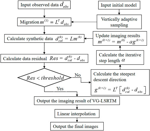
FIGURE 2. Flowchart of the proposed VG-LSRTM.

Numerical examples

In this section, we demonstrate the feasibility and advantages of the proposed method with synthetic data. The numerical tests are for two models: 1) a layered model and 2) a modified Marmousi model.

Layered model

First, we use a layered model shown in Figure 3A to illustrate the implementation process of VG-LSRTM in detail. The model is 3 km wide and 1.5 km deep, which has three horizontal layers with velocity of 1,500 m/s, 2,500 m/s and 4,500 m/s, respectively. Three comparative tests shown Table 1 are designed to demonstrate the effectiveness of our method. In Test 1, the size of the fine-grid model grids is 601 $\times$ 301 with a 5 m grid spacing. 601 $\times$ 201 grid points are used in coarse-grid model (Test 2), with grid interval of $dx=$ 5 m and $dz=$ 7.5 m. The variable-grid model is displayed in Figure 3B, which is resampled from the fine-grid model. Compared with the fine-grid model, the number of vertical grid points of the variable-grid model is reduced by 34.6%.

FIGURE 3

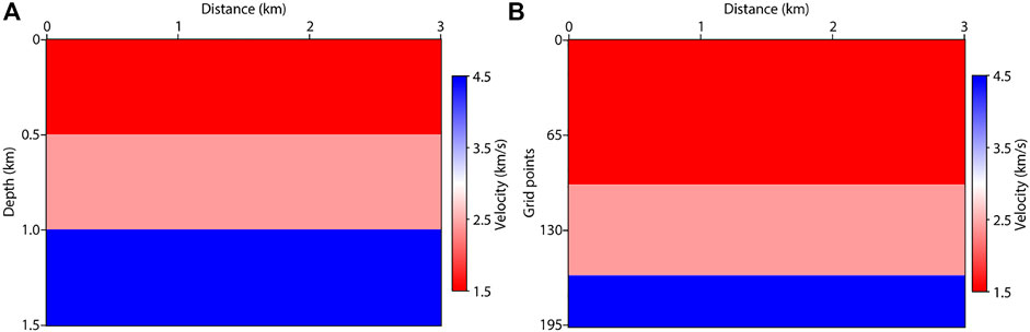
FIGURE 3. Layered model: (A) regular-grid model and (B) variable-grid model.

TABLE 1

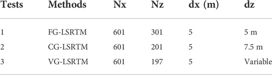
TABLE 1. Modeling parameters of FG-LSRTM, CG-LSRTM and VG-LSRTM tests.

Figure 4 shows the vertical grid spacing of these models. The blue dashed line denotes the theoretical optimal value of the fine-grid model, which is calculated by Eq. 2. The red dashed line displays the vertical grid spacing of the variable-gird model. It varies more smoothly between two layers than the blue line. For conventional variable-grid methods (Jastram and Tessmer, 1994; Wang and Schuster, 1996; Ha and Shin, 2012; Fan et al., 2015), it is inevitable to add a transition area between two layers with different velocity, change the finite-difference scheme of the seismic wave equation, or modify the finite-difference coefficients. When the modeling parameters are not reasonable, strong spurious reflections will occur in the transition area. Our adaptive variable-grid method is much easier to implement and can effectively avoid the spurious reflections.

FIGURE 4

FIGURE 4. Comparison of vertical grid interval.

Next, we test our method using forward modeling. A Ricker wavelet source with dominant frequency of 30 Hz is used. The time step is 0.5 ms. Figures 5A–C show the wavefield snapshots at 0.65 s, which are computed by the fine-grid, coarse-grid and variable-grid methods, respectively. The variable-grid snapshot (Figure 5C) is irregular in depth direction. For comparison purposes, we apply linear interpolation to it to get a regular-grid one, as shown in Figure 5D. As indicated by the red arrows, numerical dispersion in Figure 5B is stronger than that in Figures 5A,D. As shown in Figure 6, we extract a single trace from these snapshots at a distance of 1.3 km for further comparison. The black arrows indicate the dispersion. From Figure 6, we find that the blue line and the red line almost coincide but they are different from the black line.

FIGURE 5

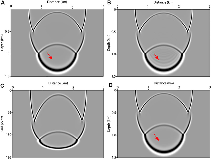
FIGURE 5. Wavefield snapshots computed by: (A) fine-grid method, (B) coarse-grid method, (C) variable-grid method, and (D) variable-grid method with linear interpolation.

FIGURE 6

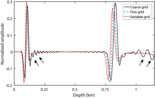
FIGURE 6. Comparison of the snapshots at a distance of 1.3 km for different forward modeling methods.

In LSRTM tests, the recording time is 1.5 s. In total, 21 shots are evenly distributed on the surface and the shot interval is 150 m. Each shot has 601 receivers and the receiver interval is 5 m. Figure 7A shows the synthetic single shot record using the fine-grid model, which is regarded as the observed data. Figures 7B–D show the Born-modeled data at the first iteration of the fine-grid method, coarse-grid method and variable-grid method, respectively. Obviously, the numerical dispersion in Figure 7C is strong (see the red arrow). Figures 8A–C show the FG-LSRTM, CG-LSRTM and VG-LSRTM images after 20 iterations, respectively. Figure 8D shows the linear interpolation profile of the image in Figure 8C. As indicated by the red arrows in Figure 8, the FG-LSRTM and VG-LSRTM images show fewer imaging artifacts, higher resolution, and better balance of reflector amplitudes compared with the CG-LSRTM image. Figure 9 shows the convergence curves of the normalized data residual. The convergence curves of FG-LSRTM method and the VG-LSRTM method almost coincide after 15 iterations, which means that the proposed algorithm converges as fast as conventional LSRTM.

FIGURE 7

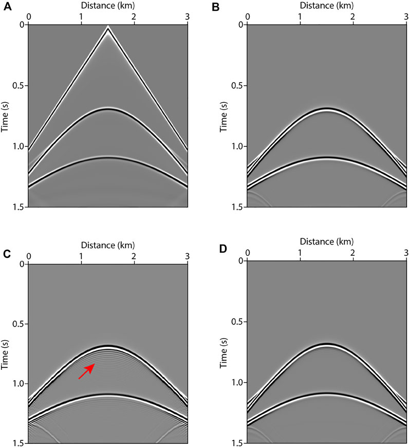
FIGURE 7. Single shot record: (A) observed data, (B) Born-modeled data at the first iteration of the fine-grid test, (C) Born-modeled data at the first iteration of the coarse-grid test, and (D) Born-modeled data at the first iteration of the variable-grid test.

FIGURE 8

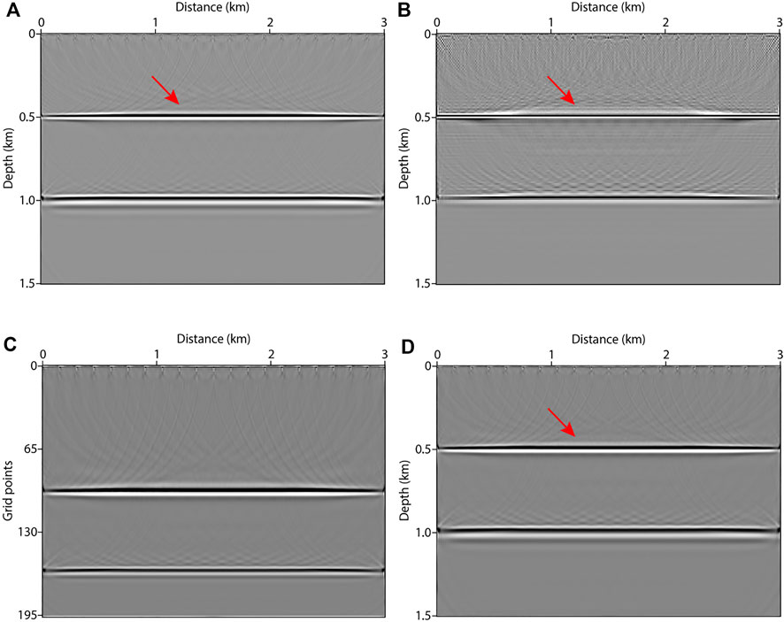
FIGURE 8. LSRTM images after 20 iterations: (A) FG-LSRTM image, (B) CG-LSRTM image, (C) VG-LSRTM image, and (D) VG-LSRTM image after linear interpolation.

FIGURE 9

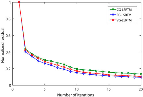
FIGURE 9. Normalized data residual convergence curves of the three LSRTM tests.

These LSRTM tests are performed on a cluster using twenty-one server nodes. The CPU is a 2.20 GHz Intel Xeon Silver 4,214, which has forty-five compute nodes. The computing time of FG-LSRTM, CG-LSRTM and VG-LSRTM is 93 min, 62 min and 64 min, respectively. The VG-LSRTM method saves about 34.6% of memory compared to the FG-LSRTM method because the number of vertical grid of the variable-grid model is 34.6% of that of the fine-grid model. From the layered model tests, we conclude that the VG-LSRTM method can improve computing efficiency, reduce memory consumption, and provide high-resolution image with little accuracy loss.

Modified Marmousi model

Similar to the previous section, we use the coarse-grid, fine-grid, and variable-grid Marmousi models to further verify the advantages of the proposed method. The model parameters are shown in Table 2. Figure 10A shows the regular-grid model. Figure 10B displays the variable-grid model, which is resampled from the fine-grid model. From Table 2, the number of vertical grid points of the variable-grid model is 360, decreasing by 48.6%. The comparison of vertical grid interval is presented in Figure 11. We can see that the variable-grid grid interval (the red line) varies smoothly with model velocity.

TABLE 2

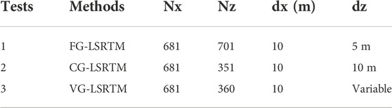
TABLE 2. Model parameters of FG-LSRTM, CG-LSRTM and VG-LSRTM tests.

FIGURE 10

FIGURE 10. Modified Marmousi model: (A) regular-grid model, and (B) variable-grid model.

FIGURE 11

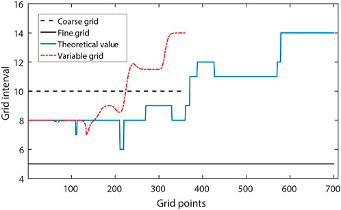
FIGURE 11. Comparison of vertical grid interval.

In imaging tests, the time interval is 0.3 ms, and the recording time is 3 s. In total, 35 sources are distributed laterally from 0 to 6.65 km, and the shot interval is 200 m. Each shot has 681 receivers, and the receiver interval is 10 m. The dominant frequency of the Ricker wavelet source is 30 Hz. Figure 12 shows the images after 30 iterations. Figure 12A displays the FG-LSRTM image, Figure 12B shows the CG-LSRTM image, Figure 12C shows the VG-LSRTM image, and Figure 12D shows the VG-LSRTM image after linear interpolation. Figure 13 shows the magnified views of the dashed red boxes shown in Figure 12. Obviously, the images in Figures 13A,C show better imaging resolution than that in Figure 13B. To demonstrate that the VG-LSRTM method has high accuracy and low errors, we extract two traces from the images in Figures 13A,C (see the red and blue lines). Figures 14A,B show the single trace comparison at the distance of 3.5 km and 4.25 km, respectively. We can see that there is almost no amplitude and phase error between the FG-LSRTM and the VG-LSRTM image.

FIGURE 12

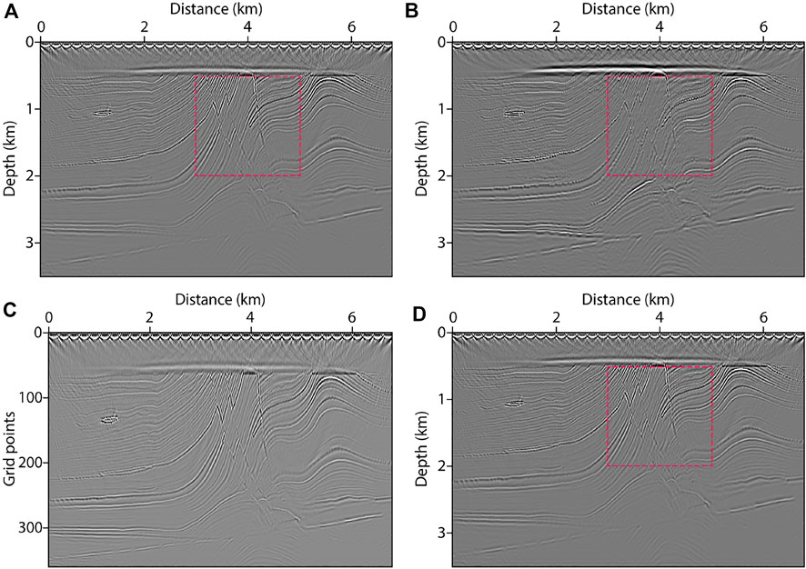
FIGURE 12. LSRTM images using different migration velocity model after 30 iterations: (A) FG-LSRTM image, (B) CG-LSRTM image, (C) VG-LSRTM image, and (D) VG-LSRTM image after linear interpolation.

FIGURE 13

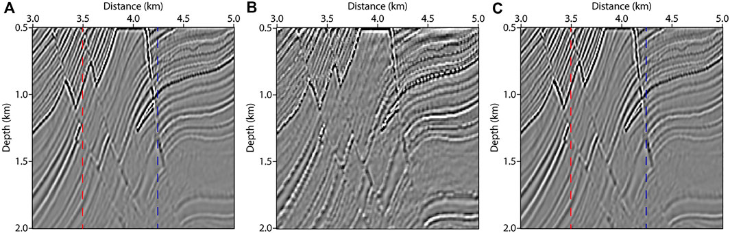
FIGURE 13. Magnified views of the dashed red boxes shown in Figure 12: (A) FG-LSRTM image, (B) CG-LSRTM image, and (C) VG-LSRTM image after linear interpolation.

FIGURE 14

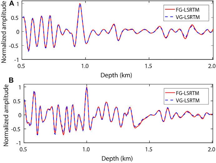
FIGURE 14. Vertical slices of Figure 13 at: (A) 3.5 km and (B) 4.25 km.

Figure 15 shows the normalized data residual convergence curves of these tests. We can see that the curves of the FG-LSRTM method and the VG-LSRTM method almost coincide, and they converge faster than that of the CG-LSRTM method. Each LSRTM test uses thirty-five nodes on a 2.20 GHz Intel Xeon Silver 4214 CPU. The computing time of FG-LSRTM, CG-LSRTM and VG-LSRTM is 25.6 h, 13.1 h and 13.8 h, respectively. Compared with the FG-LSRTM method, our VG-LSRTM method can save 46% of the computation time. From the numerical example of the modified Marmousi model, we conclude that the proposed VG-LSRTM method can greatly improve computing efficiency.

FIGURE 15

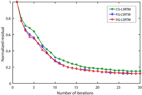
FIGURE 15. Normalized data residual convergence curves of CG-LSRTM, FG-LSRTM and VG-LRSRTM methods.

Discussion

Numerical tests on the layered model and the modified Marmousi model have shown that the proposed method is efficient and accurate. Nevertheless, the final effect that our method can achieve depends on initial spatial grid interval, the velocity structure of the model, and the maximum frequency of the source. Severe vertical velocity variation, small spatial grid interval, and the use of low-frequency source are favorable factors for the proposed VG-LSRTM algorithm. In addition, the accuracy loss of VG-LSRTM images mainly originates from the sampling process shown in Figure 1 because model velocity varies continuously while the grid points are obtained by discrete sampling. Other factors that may reduce the accuracy of the imaging results, such as the use of linear interpolation technology and the order of the finite-difference scheme for approximating $\phi \left(z\right)$, have negligible effects on the final results. The stability condition of Eq. 4 is worth discussing. By analyzing the results of a large number of numerical tests, we find that the stability condition of Eq. 4 is slightly more stringent than that of Eq. 1.

Conclusion

Conventional variable-grid methods are difficult to implement and apply to LSRTM. We presented a VG-LSRTM algorithm based on an adaptive sampling strategy to accelerate LSRTM in this paper. We derived a variable-grid first-order stress-velocity acoustic wave equation and its corresponding Born forward modeling operator based on a mapping relationship between two coordinate systems. We developed a complete VG-LSRTM workflow and proved its feasibility using two numerical examples. Forward modeling tests for a layered model demonstrated that the proposed variable-grid method has high wavefield simulation accuracy. LSRTM tests for the layered model and a modified Marmousi model validated that our VG-LSRTM can save large computing costs and provide high-resolution imaging results as well as FG-LSRTM.

Data availability statement

The original contributions presented in the study are included in the article/Supplementary Material, further inquiries can be directed to the corresponding authors.

Author contributions

LC and JH contributed to the conception and design of the study. CS and JH organized the database and performed the statistical analysis. ZW modified the manuscript. All authors contributed to manuscript revision and read and approved the submitted version.

Funding

This research is supported by the Marine S&T Fund of Shandong Province for Pilot National Laboratory for Marine Science and Technology (Qingdao) (Grant No. 2021QNLM020001), the National Key R&D Program of China (Grant No. 2019YFC0605503C), and the National Outstanding Youth Science Foundation (Grant No. 41922028).

The authors declare that this study received funding from the Major Scientific and Technological Projects of China National Petroleum Corporation (CNPC) (grant no. ZD2019-183-003). The funder was not involved in the study design, collection, analysis, interpretation of data, the writing of this article, or the decision to submit it for publication.

Acknowledgments

We are grateful to the editor and the reviewers for reviewing this manuscript.

Conflict of interest

The authors declare that the research was conducted in the absence of any commercial or financial relationships that could be construed as a potential conflict of interest.

Publisher’s note

All claims expressed in this article are solely those of the authors and do not necessarily represent those of their affiliated organizations, or those of the publisher, the editors and the reviewers. Any product that may be evaluated in this article, or claim that may be made by its manufacturer, is not guaranteed or endorsed by the publisher.

References

Alkhalifah, T. (2003). Tau migration and velocity analysis: Theory and synthetic examples. Geophysics 68 (4), 1331–1339. doi:10.1190/1.1598126

CrossRef Full Text | Google Scholar

Baysal, E., Kosloff, D. D., and Sherwood, J. W. C. (1983). Reverse time migration. Geophysics 48 (11), 1514–1524. doi:10.1190/1.1441434

CrossRef Full Text | Google Scholar

Buur, J., and Kühnel, T. (2008). Salt interpretation enabled by reverse-time migration. Geophysics 73 (5), VE211–VE216. doi:10.1190/1.2968690

CrossRef Full Text | Google Scholar

Chen, Y., Dutta, G., Dai, W., and Schuster, G. T. (2017). Q-least-squares reverse time migration with viscoacoustic deblurring filters. Geophysics 82 (6), S425–S438. doi:10.1190/geo2016-0585.1

CrossRef Full Text | Google Scholar

Claerbout, J. F. (1971). Toward a unified theory of reflector mapping. Geophysics 36, 467–481. doi:10.1190/1.1440185

CrossRef Full Text | Google Scholar

Dai, W., Fowler, P., and Schuster, G. T. (2012). Multi-source least-squares reverse time migration. Geophys. Prospect. 60 (4), 681–695. doi:10.1111/j.1365-2478.2012.01092.x

CrossRef Full Text | Google Scholar

Dai, W., and Schuster, G. T. (2013). Plane-wave least-squares reverse-time migration. Geophysics 78 (4), S165–S177. doi:10.1190/geo2012-0377.1

CrossRef Full Text | Google Scholar

Dai, W., Wang, X., and Schuster, G. T. (2011). Least-squares migration of multisource data with a deblurring filter. Geophysics 76 (5), R135–R146. doi:10.1190/geo2010-0159.1

CrossRef Full Text | Google Scholar

Díaz, E., and Sava, P. (2016). Understanding the reverse time migration backscattering: Noise or signal? Geophys. Prospect. 64, 581–594. doi:10.1111/1365-2478.12232

CrossRef Full Text | Google Scholar

Dong, S., Cai, J., Guo, M., Suh, S., Zhang, Z., Wang, B., et al. (2012). Least squares reverse time migration towards true amplitude imaging and improving the resolution. 82nd Annu. Int. Meet. Seg. Expand, 1–5. doi:10.1190/segam2012-1488.1

CrossRef Full Text | Google Scholar

Du, Q. Z., Guo, C. F., Zhao, Q., Gong, X. F., Wang, C. X., and Li, X. Y. (2017). Vector-based elastic reverse time migration based on scalar imaging condition. Geophysics 82 (2), S111–S127. doi:10.1190/geo2016-0146.1

CrossRef Full Text | Google Scholar

Duprat, V., and Baina, R. (2016). An efficient least-squares reverse-time migration using true-amplitude imaging condition as an optimal preconditioner. 78th Annu. Int. Conf. Exhib. EAGE, Ext. Abstr, 1–5. doi:10.3997/2214-4609.201601199

CrossRef Full Text | Google Scholar

Dutta, G., and Schuster, G. T. (2014). Attenuation compensation for least-squares reverse time migration using the viscoacoustic-wave equation. Geophysics 79 (6), S251–S262. doi:10.1190/geo2013-0414.1

CrossRef Full Text | Google Scholar

Falk, J., Tessmer, E., and Gajewski, D. (1996). Tube wave modeling by the finite-difference method with varying grid spacing. PAGEOPH 148, 77–93. doi:10.1007/BF00882055

CrossRef Full Text | Google Scholar

Fan, N., Zhao, L. F., Gao, Y. J., and Yao, Z. X. (2015). A discontinuous collocated-grid implementation for high-order finite-difference modeling. Geophysics 80 (4), T175–T181. doi:10.1190/geo2015-0001.1

CrossRef Full Text | Google Scholar

Feng, Z. C., and Schuster, G. T. (2017). Elastic least-squares reverse time migration. Geophysics 82 (2), S143–S157. doi:10.1190/geo2016-0254

CrossRef Full Text | Google Scholar

Gu, B., Li, Z., and Han, J. (2018). A wavefield-separation-based elastic least-squares reverse time migration. Geophysics 83 (3), S279–S297. doi:10.1190/geo2017-0131.1

CrossRef Full Text | Google Scholar

Ha, W., and Shin, C. (2012). Efficient Laplace-domain modeling and inversion using an axis transformation technique. Geophysics 77 (4), R141–R148. doi:10.1190/geo2011-0424.1

CrossRef Full Text | Google Scholar

Hill, N. R. (1990). Gaussian beam migration. Geophysics 55, 1416–1428. doi:10.1190/1.1442788

CrossRef Full Text | Google Scholar

Hu, H., Liu, Y., Zheng, Y., Liu, X., and Lu, H. (2016). Least-squares Gaussian beam migration. Geophysics 81 (3), S87–S100. doi:10.1190/geo2015-0328/1

CrossRef Full Text | Google Scholar

Jastram, C., and Behle, A. (1992). Acoustic modelling on a grid of vertically varying Spacing1. Geophys. Prospect. 40 (2), 157–169. doi:10.1111/j.1365-2478.1992.tb00369.x

CrossRef Full Text | Google Scholar

Jastram, C., and Tessmer, E. (1994). Elastic modelling on a grid with vertically varying spacing1. Geophys. Prospect. 42 (4), 357–370. doi:10.1111/j.1365-2478.1994.tb00215.x

CrossRef Full Text | Google Scholar

Kristian, T., and Mauricio, S. (2022). Least-squares reverse time migration via deep learning-based updating operators. Geophysics 87 (6), S315–S333. doi:10.1190/geo2021-0491.1

CrossRef Full Text | Google Scholar

Kühl, H., and Sacchi, M. D. (2003). Least-squares wave-equation migration for AVP/AVA inversion. Geophysics 68, 262–273. doi:10.1190/1/1543212

CrossRef Full Text | Google Scholar

Lailly, P., and Bednar, J. (1983). The seismic inverse problem as a sequence of before stack migrations. Conf. Inverse Scatt. Theory Appl., 206–220.

Google Scholar

Lambaré, G., Virieux, J., Madariaga, R., and Jin, S. (1992). Iterative asymptotic inversion in the acoustic approximation. Geophysics 57, 1138–1154. doi:10.1190/1.1443328

CrossRef Full Text | Google Scholar

Li, C., Gao, J. H., Gao, Z. Q., Wang, R. R., and Yang, T. (2020). Periodic plane-wave least-squares reverse time migration for diffractions. Geophysics 85 (4), S185–S198. doi:10.1190/geo2019-0211.1

CrossRef Full Text | Google Scholar

Li, C., Huang, J., Li, Z., and Wang, R. (2018). Plane-wave least-squares reverse time migration with a preconditioned stochastic conjugate gradient method. Geophysics 83, S33–S46. doi:10.1190/geo2017-0339.1

CrossRef Full Text | Google Scholar

Li, Q., Huang, J., and Li, Z. (2017). Cross-correlation least-squares reverse time migration in the pseudo-time domain. J. Geophys. Eng. 14 (4), 841–851. doi:10.1088/1742-2140/aa6B33

CrossRef Full Text | Google Scholar

Li, Z., Li, Q., Huang, J., Na, L., and Kun, T. (2014). A stable and high-precision dual-variable grid forward modeling and reverse time migration method. Geophys Prospect Pet. 53 (2), 127–136. doi:10.3969/j.issn.1000-1441.2014.02.001

CrossRef Full Text | Google Scholar

Liu, X., and Liu, Y. (2018). Plane-wave domain least-squares reverse time migration with free-surface multiples. Geophysics 83 (6), S477–S487. doi:10.1190/geo2017-0570.1

CrossRef Full Text | Google Scholar

Ma, X., and Alkhalifah, T. (2013). Wavefield extrapolation in pseudodepth domain. Geophysics 78 (2), S81–S91. doi:10.1190/geo2012-0237.1

CrossRef Full Text | Google Scholar

Moczo, P. (1989). Finite-difference technique for SH-waves in 2-D media using irregular grids-application to the seismic response problem. Geophys. J. Int. 99 (2), 321–329. doi:10.1111/j.1365-246X.1989.tb01691.x

CrossRef Full Text | Google Scholar

Mu, X., Huang, J. P., Yang, J. D., Guo, X., and Guo, Y. D. (2020). Least-squares reverse time migration in TTI media using a pure qP-wave equation. Geophysics 85 (4), S199–S216. doi:10.1190/geo2019-0320.1

CrossRef Full Text | Google Scholar

Nemeth, T., Wu, C., and Schuster, G. T. (1999). Least-squares migration of incomplete reflection data. Geophysics 64 (1), 208–221. doi:10.1190/1.1444517

CrossRef Full Text | Google Scholar

Qu, Y., Huang, J. P., Li, Z. C., Guan, Z., and Li, J. L. (2017). Attenuation compensation in anisotropic least-squares reverse time migration. Geophysics 82 (6), S411–S423. doi:10.1190/geo2016-0677.1

CrossRef Full Text | Google Scholar

Ren, Z., Liu, Y., and Sen, M. K. (2017). Least-squares reverse time migration in elastic media. Geophys. J. Int. 208, 1103–1125. doi:10.1093/gji/ggw443

CrossRef Full Text | Google Scholar

Rocha, D., Sava, P., and Guitton, A. (2018). 3D acoustic least-squares reverse time migration using the energy norm. Geophysics 83 (3), S261–S270. doi:10.1190/geo2017-0466.1

CrossRef Full Text | Google Scholar

Rocha, D., Tanushev, N., and Sava, P. (2016). Acoustic wavefield imaging using the energy norm. Geophysics 81 (4), S151–S163. doi:10.1190/geo2015-0486.1

CrossRef Full Text | Google Scholar

Schneider, W. A. (1978). Integral formulation for migration in two and three dimensions. Geophysics 43, 49–76. doi:10.1190/1.1440828

CrossRef Full Text | Google Scholar

Sun, J., Fomel, S., Zhu, T., and Hu, J. (2016). Q-compensated least-squares reverse time migration using low-rank one-step wave extrapolation. Geophysics 81 (4), S271–S279. doi:10.1190/geo2015-0520.1

CrossRef Full Text | Google Scholar

Sun, R., and McMechan, G. A. (2001). Scalar reverse-time depth migration of prestack elastic seismic data. Geophysics 66, 1519–1527. doi:10.1190/1/1487098

CrossRef Full Text | Google Scholar

Sun, X. D., Li, Z. C., and Jia, Y. R. (2017). Variable-grid reverse-time migration of different seismic survey data. Appl. Geophys. 14 (4), 517–522. doi:10.1007/s11770-017-0652-7

CrossRef Full Text | Google Scholar

Tan, S., and Huang, L. J. (2014). Least-squares reverse-time migration with a wavefield separation imaging condition and updated source wavefields. Geophysics 79 (5), S195–S205. doi:10.1/1190/geo2014/0020/1

CrossRef Full Text | Google Scholar

Vamaraju, J., Vila, J., Araya-Polo, M., Datta, D., Sidahmed, M., and Sen, M. K. (2021). Minibatch least-squares reverse time migration in a deep-learning framework. Geophysics 86 (2), S125–S142. doi:10.1190/geo2019-0707/1

CrossRef Full Text | Google Scholar

Virieux, J. (1986). P-SV wave propagation in heterogeneous media: Velocity-stress finite-difference method. Geophysics 51, 889–901. doi:10.1190/1.1442147

CrossRef Full Text | Google Scholar

Wang, P., Huang, S., and Wang, M. (2017). Improved subsalt images with least-squares reverse time migration. Interpretation 5 (3), SN25–SN32. doi:10.1190/INT-2016-0203.1

CrossRef Full Text | Google Scholar

Wang, Y., and Schuster, G. T. (1996). Finite-difference variable grid scheme for acoustic and elastic wave equation modeling. Seg. Tech. Program Expand. Abstr. 15, 674–677. doi:10.1190/11826737

CrossRef Full Text | Google Scholar

Wang, Y. (2001). Viscoelastic wave simulation in basins by a variable grid finite difference method. Bull. Seismol. Soc. Am. 91 (6), 1741–1749. doi:10.1785/0120000236

CrossRef Full Text | Google Scholar

Whitmore, N. D. (1983). Iterative depth migration by backward time propagation. In 53rd Annual International Meeting, SEG, Expanded Abstracts, 382–385. doi:10.1190/1.1893867

CrossRef Full Text | Google Scholar

Xie, X. B., and Wu, R. S. (2005). Multicomponent prestack depth migration using the elastic screen method. Geophysics 70 (1), S30–S37. doi:10.1190/1/1852787

CrossRef Full Text | Google Scholar

Xue, H., and Liu, Y. (2017). Multi-source least-square reverse time migration based on MPI and CUDA hybrid accelerating algorithm. In 79th EAGE Conference and Exhibition. Paris, France, 1–5. doi:10.3997/2214-4609.201701126

CrossRef Full Text | Google Scholar

Yang, J., Zhu, H., McMechan, G., Zhang, H. Z., and Zhao, Y. (2019). Elastic least-squares reverse time migration in vertical transverse isotropic media. Geophysics 84 (6), S539–S553. doi:10.1190/geo2018-0887.1

CrossRef Full Text | Google Scholar

Yang, J., and Zhu, H. (2019). Viscoacoustic least-squares reverse-time migration using a time-domain complex-valued wave equation. Geophysics 84 (5), S479–S499. doi:10.1190/geo2018-0804.1

CrossRef Full Text | Google Scholar

Yilmaz, O. (2001). Seismic data analysis: Processing, inversion, and interpretation of seismic. Tulsa, Oklahoma, USA: Society of Exploration Geophysicists, doi:10.1190/1.9781560801580

CrossRef Full Text | Google Scholar

Zhang, Q., Mao, W., and Chen, Y. (2018). Attenuating crosstalk noise of simultaneous-source least-squares reverse time migration with gpu-based excitation amplitude imaging condition. IEEE Trans. Geosci. Remote Sens. 57, 587–597. doi:10.1109/TGRS.2018.2858850

CrossRef Full Text | Google Scholar

Zhang, Y., Duan, L., and Yi, X. (2015). A stable and practical implementation of least-squares reverse time migration. Geophysics 80 (1), V23–V31. doi:10.1190/segam2013-0577.1

CrossRef Full Text | Google Scholar

Zhang, Y., and Sun, J. (2009). Practical issues of reverse time migration: True amplitude gathers, noise removal and harmonic-source encoding. Proceedings of the Beijing International Geophysical Conference and Exposition, Beijing, China, 204.

CrossRef Full Text | Google Scholar

Zhao, Z., and Sen, M. K. (2019). Frequency-domain double-plane-wave least-squares reverse time migration. Geophys. Prospect. 67, 2061–2084. doi:10.1111/1365-2478.12803

CrossRef Full Text | Google Scholar