DL-KF modeling for acceleration of flash calculations in phase equilibrium using deep learning methods

Improving the robustness and efficiency of flash calculations in phase equilibrium is crucial for reservoir simulation. DL-KF (Deep Learning for K-values and Fugacity Calculation) modeling is proposed to accelerate phase equilibrium calculation using deep learning methods, in which the three-steps neural networks are included: ANN-STAB (Artificial Neural Network for Stability Test) model, ANN-KV (Artificial Neural Network for K-values Calculation) model and ANN-FUG (Artificial Neural Network for Fugacity Calculation) model respectively. The ANN-STAB model is generated to test phase stability. When temperature, pressure and feed composition are given, the phase classification is obtained directly with very low computation cost. In the ANN-KV model, initial K-values are determined by trained networks instead of employing Wilson equation employed in traditional flash calculation. Its initial estimations of K-values significantly reduce the number of iterations and avoid converging to incorrect or unphysical solutions. The ANN-FUG model is built to replace the fugacity coefficient calculation in traditional flash calculation algorithms, and simplifies the nonlinear calculation of internal iterative calculation. These three artificial neural network models are embedded into the traditional algorithms to accelerate flash calculations. The framework considers the complete physical process of the algorithms of flash calculations in phase equilibrium calculations using deep learning methods, and it can also guarantee the conservation of component mass, which is crucial for phase equilibrium calculations and reservoir simulation. The proposed DL-KF modeling is validated and compared with the original equation of state modeling and three other deep learning methods using two typical hydrocarbon fluid cases. A sample of C₃H₈-CO₂-heavy oil systems from Huabei oilfield and a PVT experiment in Tahe oilfield are used to examine the DL-KF modeling. The physical properties of oil sample of Bakken reservoir with CO₂ injection are also investigated. These results reveal that the DL-KF methoding is accurate and efficient for accelerating phase equilibrium calculations of reservoir fluids.

1 Introduction

Compositional simulation is widely applied for designing and optimizing enhanced oil recovery (EOR) processes (Xiong, 2015; Nojabaei et al., 2016). Flash calculation based on equation of state (EOS) is employed in compositional model, which is essential for a better understanding of the mechanics of fluids flow in reservoirs (Wang and Erling, 1994). However, because of its inherent nonlinearity, it usually turns out to be unstable and high time-consuming in the determination of phase classification and composition concentrations at each grid-block and each time step (Zhu and Li, 2020). The efficiency and robustness of phase equilibrium calculation is crucial for reservoir simulation (Yang et al., 2016; Zhang et al., 2017; Liu et al., 2018a; Liu et al., 2018b).

To accelerate the computing speed and improve the stability of flash calculation, several methods have been adopted. A simple and direct acceleration strategy is to reduce the number of equations or variables. Therefore, it is evident to take advantage of the rank of the BIP matrix using only the most significant eigenvalues. Michelsen (Michelsen, 1986) first proposed a reduction method to decrease the number of nonlinear equations by taking advantage of the low-rank binary interaction parameters (BIP) matrix using only the most significant eigenvalues. Firoozabadi and Pan (Firoozabadi and Pan, 2000; Pan and Firoozabadi, 2001) developed another reduction method based on the spectral theory of linear algebra to speed up the phase stability tests and composition concentrations calculations. A smoother tangent plane distance (TPD) function can be obtained in the reduced space and robustness and efficiency of their reduction model is verified through numerical tests. Hendriks and Van Bergen (Hendriks and Van Bergen, 1992) approximated the BIP matrix based on spectral expansion and then reduce the number of eigenvectors which makes the error and the number of parameters of the BIP matrix smaller. Nichita (Nichita and Minescu, 2004; Nichita et al., 2006; Nichita and Graciaa, 2011) reduced the number of equations to be solved in flash calculations by selecting independent variables or using truncated expectral expantion of the attraction parameter of the EOS. Li and Johns (Li and Johns, 2006) implemented a reduction method by decomposing the BIP matrix into two parts using a quadratic expression. Gaganis and Varotsis (Gaganis and Varotsis, 2014) approximated the BIP matrix through the minimization of an energy function, which decomposes the BIP matrix to a set of basis vectors. These results show that the method saves computational time without losing high degree of accuracy. Another strategy is to solve the non-linear phase equilibrium equations for each gridlock separately from the reservoir simulation in order to reduce the computational costs. Belkadi et al. (Belkadi et al., 2011) proposed a Tie-line method to obtain approximate flash calculation results in a two-phase region. The method aims to use the distance to a previous Tie-line in the same grid block to decide whether an approximation should be made. Voskov and Tchelepi (Voskov and Tchelepi, 2007) proposed a compositional space parametrization approach for simulation of gas flooding processes. Flash calculations are performed and results are stored as a preprocessing stage for reservoir simulation. During the simulation, if the concentration lies on the compositional tie line, a tie-line table is used to look up the flash results. The performance of tie-line method is improved by using information from the previous time step to determine the phase state of the current step. Despite many efforts have been employed to accelerate flash calculations, they only marginally improve single aspects of the calculation by some kinds of mathematical manipulation or ignoring some complex thermodynamic procedures such as phase stability tests. Wu et al. (Wu et al., 2015) decoupled the flash calculations from the composition simulation using a sparse grid method, which shifts flash calculation from the composition simulation (online) to a pre-simulation (offline) phase. This treatment significantly reduces the computational costs. However, the detection of single-phase region is not always accurate and reliable, while the saturation can even exceed the physically meaningful boundaries. In addition, the generation of the surrogate model in sparse grid method is still time-consuming.

During the last two decades, numerous speeding up methods for flash calculation are presented, but the wide recognition, high accuracy and general application are still the focus of attention. With the rapid development of artificial intelligence (AI), deep learning methods has been widely used in the oil and gas industry (Jin et al., 2020; Sun, 2020; Mohamed et al., 2021; Wang et al., 2021; Xiao et al., 2021), flash calculation in phase equilibrium calculation included. Wang (Wang et al., 2019a) constructed a two-step neural network to proxy flash calculation. The first step neural network is to test phase stability of the system and the second step neural network is to predict the composition concentration among the determined phases. Zhang (Zhang et al., 2020) also designed two network structures, in which “Ghost components” are defined and introduced to process the data padding work in order to modify the dimension of input flash calculation data to meet the training and testing requirements of the target fluid mixture. This makes the deep learning algorithms to be self-adaptive to the change of input components and dimensions. Li (Yu et al., 2019) designed and tuned a fully connected deep neural network, in which the critical thermodynamic properties are selected as input features to represent each component implicitly. Although above mentioned methods which is a nonlinear fitting called “surrogate modeling” can accelerate flash calculation, they simply implement nonlinear fitting of input and output variables, lack rigorous thermodynamic theory basis and do not consider the constraints of mass conservation in flash calculations. In some cases, the calculation accuracy is difficult to guarantee. Moreover, the surrogate modeling could not guarantee the conservation of mass, which is crucial for reservoir simulation. Initial guesses of K-values and vapor mole fraction with good quality can speed up the convergence of two-phase flash calculation and avoid trivial solution (Vatandoost et al., 2016). If no additional data is available, Wilson’s equation is usually used to estimate K-values (Wilson, 1968). However, estimation based on this correlation is not accurate at high pressure conditions and leads to trivial solution (Wang et al., 2019b). Gaganis (Gaganis et al., 2021) proposed a new soft computing pressure-explicit, adaptive k-values interpolation technique, which can be thought as a method that generates fluid-specific regression models of the k-values as functions of pressure, temperature and the original fluid composition. During the simulation process, the so beforehand calculated equilibrium coefficients are used with the Rachford-Rice equation to determine rapidly the composition concentrations and properties of phases present, hence greatly reducing the CPU time. Wang (Wang et al., 2019b; Wang et al., 2020) developed two ANN models: an ANN-STAB model and an ANN-SPLIT model. The ANN-STAB model is built to fit a saturation pressure diagram and the ANN-SPLIT model is generated to regress K-values and mole fractions, which are to be used as initial guesses in the following phase splitting calculations. Good initial guesses of K-values and vapor mole fraction can reduce iteration numbers obviously. This approach implements “internal substitution” for deep learning methods and considers physically meanings. However, compared with the surrogate modeling, this method still solves the nonlinear equations for compressibility factors calculation and uses Gibbs free energy minimization principle to calculate fugacity coefficients in the internal iterative processes.

Therefore, A DL-KF modeling based on three-steps neural networks is designed which includes ANN-STAB model, ANN-KV model and ANN-FUG model respectively. The ANN-STAB model is generated for phase stability test. The ANN-KV model is used for initial K-values determination. The ANN-FUG model is designed for fugacity coefficient calculation. These three ANN models are embedded into the traditional algorithms to accelerate flash calculations. Compared with the surrogate modeling which simply implements nonlinear fitting of input and output variables and lacks rigorous thermodynamic theory basis, The proposed model can guarantee the conservation of compositional mass, which is crucial for phase equilibrium calculations and reservoir simulation. Besides, the DL-KF modeling can further improve the calculation efficiency in comparison to the proxy model proposed by Wang (Wang et al., 2019b; Wang et al., 2020) which still solves the nonlinear equations and calculate fugacity coefficients in the internal iterative processes. To the best of our knowledge, this is the first framework that considers the complete physical process of the algorithms of flash calculations in phase equilibrium calculations using deep learning methods, and it can guarantee the conservation of compositional mass.

The rest of the paper is organized as follows. In Section 2, the two-phase isothermal flash calculation algorithm is present to generate the training data set and testing data set. In Section 3, A DL-KF modeling based on three-steps neural networks is designed. In Section 4, the proposed DL-KF modeling is validated and compared with the original EOS modeling and three other deep learning methods on two typical fluid cases. In Section 5, the proposed model is applied in three oil samples from Huabei oilfield, Tahe oilfield and Bakken reservoir. At the end, summary and conclusions are provided in Section 6, and some suggestions for future researches are given.

2 Two-phase isothermal flash calculation algorithms

Oil and gas two-phase isothermal flash calculation algorithms incudes phase stability test and phase splitting calculations. Phase stability test is the premise of the phase splitting calculations, and it also provide a better initial guess for phase splitting calculations (Michelsen, 1982a). Phase splitting calculations determine composition concentrations in oil and gas phases (Michelsen, 1982b). The flash calculation algorithms are used to generate the training data set and testing data set for the deep learning model.

2.1 Phase stability test

The tangent plane distance (TPD) method is used to determine the phase stability. A $N_c$-component mixture of feed composition $z$ at specified temperature and pressure is considered. The necessary and sufficient condition for stability of this mixture is the Gibbs TPD function which can be expressed by

$\begin{array}{c}TPD\left(w\right)={\displaystyle \sum }_i{w}_i\left({\mu }_i\left(w\right)-{\mu }_i\left(z\right)\right)\end{array}(1)$

where $w$ is the compositions for any trial phases. ${\mu }_i$ is the chemical potential of composition $i$.

It is normally more convenient to rewrite the condition in terms of fugacity coefficients. The reduced TPD is defined by

$\begin{array}{c}TPD\left(w\right)={\displaystyle \sum }_i{w}_i\left(\mathit{ln}{w}_i+\mathit{ln}{\phi }_i\left(w\right)-\mathit{ln}{z}_i-\mathit{ln}{\phi }_i\left(z\right)\right)\end{array}(2)$

where ${\phi }_i$ is the fugacity coefficient of component $i$.

In order to verify phase stability, the reduced TPD must be guaranteed to be non-negative for all valid phase compositions and for all phase models in consideration. A detailed description of the numerical scheme can be found in reference (Nichita et al., 2007).

2.2 Phase splitting calculations

According to the thermodynamic theory, for a system containing $N_c$ components, the thermodynamic condition for phase equilibrium state is that when the temperature and pressure of each phase are equal, the chemical potential or fugacity of each component is equal.

$\begin{array}{c}{f}_i^L\left(T,P,x_i\right)=f_i^V\left(T,P,y_i\right)i=\mathrm{1,2},\cdots ,N_c\end{array}(3)$

$\begin{array}{c}{f_i^L=x_i\phi }_i^{L}P\end{array}(4)$

$\begin{array}{c}{f_i^V=y_i\phi }_i^{V}P\end{array}(5)$

where $f_i^L$ and $f_i^V$ are fugacity of component $i$ in the liquid and vapor phase, respectively. $x_i$ and $y_i$ are mole fraction of component $i$ in the liquid and vapor phase, respectively. $T$ is the system temperature. $P$ is the system pressure. ${\phi }_i^L$ and ${\phi }_i^V$ are fugacity coefficient of component $i$ in the liquid and vapor phase. $N_c$ is the number of components.

According to mass balance equation, Rachford and Rice (Rachford and Rice, 1952) proposed an equation to determine the equilibrium phase composition and mole fraction of component in liquid and gas phase. The mass balance equation and Rachford-Rice equation are presented in Eqs 6–8.

$\begin{array}{c}{\displaystyle \sum }_{i=1}^{N_c}{x}_i={\displaystyle \sum }_{i=1}^{N_c}{y}_i=1i=\mathrm{1,2},\cdots ,N_c\end{array}(6)$

$\begin{array}{c}{z}_i=\left(1-n_V\right)x_i+n_V{y}_i\end{array}(7)$

$\begin{array}{c}{\displaystyle \sum }_{i=1}^{N_c}\frac{\left(K_i-1\right)z_i}{1+n_V\left(K_i-1\right)}=0i=\mathrm{1,2},\cdots ,N_c\end{array}(8)$

where $z_i$ is overall mole fraction of component $i$. $n_V$ is overall number of moles in vapor phase. $K_i$ is phase equilibrium ratio of component $i$.

The initial guess of the phase equilibrium ratio of component $i$ is calculated by Wilson’s equation (Wilson, 1964).

$\begin{array}{c}{K}_i^0=\frac{P_{ci}}{P}\exp \left(5.37\left(1+{\omega }_i\right)\left(1-\frac{T_{ci}}{T}\right)\right)\end{array}(9)$

where $K_i^0$ is the initial guess of the equilibrium ratio. $P$ is system pressure. $T$ is system temperature. $P_{ci}$ and $T_{ci}$ represent the critical pressure and critical temperature of component $i$. ${\omega }_i$ is acentric factor.

The PR-EOS is adopted to calculate the fugacity coefficients (Peng and Robinson, 1972). The details of algorithms refer to Appendix.

Successive substitution and Newton-Raphson method are applied for solving nonlinear equations. Figure 1 demonstrates the flow chart for the flash calculation algorithms in phase equilibrium. The details of two-phase flash calculation algorithms are as follows:

Step 1: Assume an initial K-value for each component in the fluid mixture at the specified system pressure and temperature using Wilson’s equation.

Step 2: Test phase stability using Michelsen’s method (Michelsen, 1986). If only one phase exists in the mixture, the calculation results are output directly. If both gas and liquid phases are present, the flash calculations are performed.

Step 3: Using the overall feed compositions $z_i$ and the assumed K-values, perform flash calculations to determine liquid mole fraction $n_L$, vapor mole fraction $n_V$, each component fraction in liquid phase $x_i$ and each component fraction in liquid phase $y_i$.

Step 4: Using the calculated composition concentrations $x_i$ and $y_i$ respectively, determine the fugacity coefficient for each component in the liquid phase ${\phi }_i^L$ and vapor phase ${\phi }_i^V$ by applying Eq. A.15 and Eq. A.16.

Step 5: According to the convergence criterion, judge whether the two phases of liquid and vapor reach the state of phase equilibrium. If the phase equilibrium state is reached, the calculation results are output, otherwise the iterative loop is entered until convergence. Here the convergence tolerance $\epsilon$ sets ${10}^{-8}$.

$\begin{array}{c}{\displaystyle \sum }_{i=1}^{N_c}\left(1-\frac{f_i^L}{f_i^V}\right)<\epsilon \end{array}(10)$

$\begin{array}{c}{f}_i^L={\phi }_{\mathrm{i}}^{\mathrm{L}}{x}_{i}P\end{array}(11)$

$\begin{array}{c}{f}_i^v={\phi }_{\mathrm{i}}^{\mathrm{V}}{y}_{i}P\end{array}(12)$

where $f_i^L$ and $f_i^V$ are fugacity for each component in the liquid phase and vapor phase, respectively.

Step 6: Determine the new set of K-values from

$\begin{array}{c}{K}_i^{new}=\frac{f_i^L}{f_i^V}{K}_i\end{array}(13)$

FIGURE 1

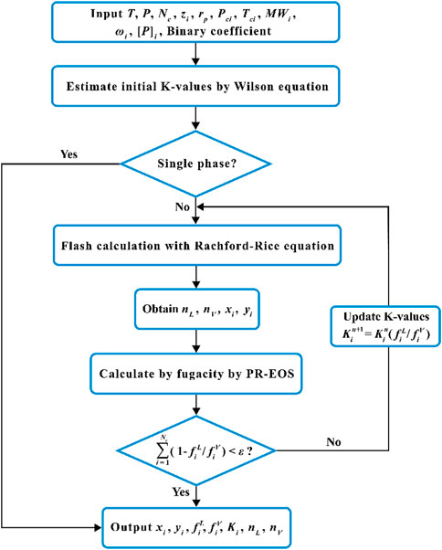
FIGURE 1. Flow char for two-phase flash calculations with PR-EOS.

3 The DL-KF modeling for accelerating flash calculations

A data-driven flash calculation algorithm named DL-KF modeling based on deep learning methods is proposed to improve the speed and convergence performance of the flash calculations in the phase equilibrium calculation.

3.1 Algorithms for the DL-KF modeling

Three important parts including phase stability test, K-values estimation and fugacity coefficients calculation affect the computational efficiency of flash calculation. In the traditional flash calculations, the phase stability test is considered as the most time-consuming part (Wang et al., 2019b). Successive Substitution Method (SSM) adopted for phase stability test may increase the iteration numbers, and the divergence may occur in the vicinity of the phase stability test limit locus (STLL) (Nichita et al., 2007). Besides, Wilson’s equation usually used to estimate K-values is not accurate at high pressure and high temperature conditions and leads to trivial solution. Furthermore, the fugacity coefficients calculation involves complex nonlinear calculations where bisection method or newton iterative algorithm is usually used. Motivated by these points, a DL-KF modeling is proposed which includes ANN-STAB model, ANN-KV model and ANN-FUG model respectively. The ANN-STAB model is developed to test phase stability instead of SSM. The ANN-KV model is constructed instead of Wilson’s equation to give an accurate initial K-values, and then improve the efficiency of the algorithm. The ANN-FUG model is generated instead of bisection method or newton iterative algorithm to determine the fugacity coefficients of fluid components. These three ANN models are embedded into the traditional algorithms to accelerate flash calculations. The schematic diagram of the DL-KF modeling for accelerating flash calculations based on deep learning methods and traditional flash calculation algorithms is shown in Figure 2.

FIGURE 2

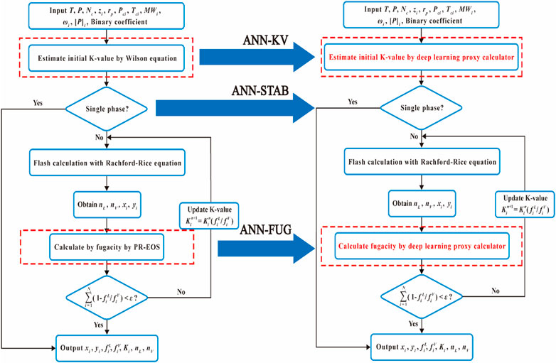
FIGURE 2. The schematic diagram of the DL-KF modeling and traditional flash calculation algorithms.

3.2 Deep learning algorithms

Each artificial neural network (ANN) model has an input layer, an output layer, and several hidden layers. Within each layer, there are several neurons. All neurons belonged to two neighboring layers are fully connected, as shown in Figure 3A. The conceptual model for the simulation process in each node is shown in Figure 3B.

FIGURE 3

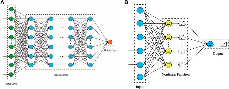
FIGURE 3. Conceptual model for the fully connected neural network (A) and the simulation process in each node (B).

Formally, for the ith hidden layer, let $a_i$ denote the input of the layer, and $c_i$ denote the output of the layer. Then:

$\begin{array}{c}{c}_i=f_i\left(W_i*a_i+b_i\right)\end{array}(14)$

where $W_i$ is the weight; $b_i$ is the bias; and $f_i$ is the activation functions of the ith layer. For a network with multiple layers, the output of one hidden layer is the input of the next layer. If the deep learning model with two hidden layers, then the output can be expressed as follow. A detailed theories for the neural networks can be found in (Bishop, 2006; LeCun et al., 2015).

$\begin{array}{c}c=f_3\left(W_3*f_2\left(W_2*f_1\left(W_2*a_1\right)+b_2\right)+b_3\right)\end{array}(15)$

3.3 Data preparation for deep learning models

To construct the configuration with the best performance with independent data, big data sets must be prepared before neural network training. Taking the data which will be described in Section 4.1 as data sets. The data sets including training data set, validation data set and testing data set are generated by solving the two-phase isothermal flash calculation. The training data set is used to adjust the weights that conform to the network architecture to produce the desired output. The validation data set is applied to tune hyperparameters which include the number of layers in the deep learning models and the number of neurons in each layer. The testing data set is used to evaluate the performance of trained model. In this paper, the data sets are divided into 80% training data, 10% verification data and 10% test data.

3.4 Training details for deep learning models

In the fully connected neural networks generated in this work, the activation function for the hidden layer and output layer is ReLU function as follows. The stochastic gradient descent (SGD) algorithm is used to train the networks. The algorithm of SGD can be briefly described in literature (Bottou, 2010).

$\begin{array}{c}\mathrm{R}\mathrm{e}\mathrm{L}\mathrm{U}\left(x\right)=\{\begin{array}{c}0\mathrm{f}\mathrm{o}\mathrm{r}x<0\\ x\mathrm{f}\mathrm{o}\mathrm{r}x\ge 0\end{array}\end{array}(16)$

In order to determine the configurations of the ANN-STAB model, ANN-KV model and ANN-FUG model, different numbers of hidden layers for the neural networks and the numbers of nodes in hidden layers are compared. Because the configuration of these three neural network models adopted in this work is the same, taking ANN-STAB model as an example for convenient description, the performance comparison of the deep learning neural networks using different number of hidden layers with the corresponding CPU time is shown in Figure 4. The results show that the CPU time increase as the number of hidden layers increases. An interesting finding is that more layers cannot ensure a lower mean squared relative error (MSRE) of liquid and vapor phase mole fractions in the model trained for phase equilibrium prediction. As shown in Figure 4, there is an obvious decreasing trend in the MSRE when the number of hidden layers increase from 1 to 2. However, it is surprising to see that the MSRE will increase slightly with the raising of layer numbers for more than 2. To achieve a better balance between accuracy and efficiency, the number of hidden layers is determined to be 2.

FIGURE 4

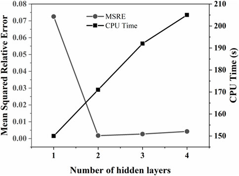
FIGURE 4. The performance comparison of the deep learning neural networks using different number of hidden layers with the corresponding CPU time.

The performance comparison of the deep learning neural networks using different number of nodes in the hidden layers is shown in Figure 5. The results show that the MSRE decreases obviously when the number of nodes increases from 10 to 30, For 40 to 60 nodes, only a very slight difference can be seen in the MSRE. An interesting finding can also be seen that when the number of nodes increases from 30 to 40, the MSRE increases slightly. To achieve a better balance between accuracy and efficiency, the number of nodes in hidden layers is determined to be 30.

FIGURE 5

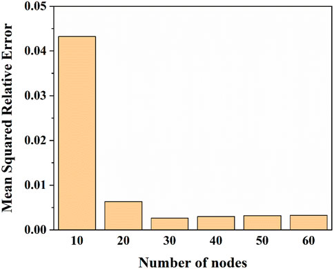
FIGURE 5. The performance comparison of the deep learning neural networks using different number of nodes in the hidden layers.

The variation of the loss function in the process of training is presented in Figure 6. As illustrated in Figure 6, the loss function of the model during the training process decreases sharply at first and then levels off as the epoch increases. Therefore, 20 epoches are adopted to train the neural networks.

FIGURE 6

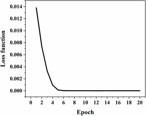
FIGURE 6. The variation of the loss function of the deep learning models during the training process.

3.5 Summary for the three ANN models

The network of these three ANN models consists of four layers, the input layer, two hidden layers and the output layer included. The dimension of two hidden layers is 30. The input parameters of three ANN model are all the system pressure and the feed composition. The output parameters are the vapor phase mole fraction, the K-values, and the fugacity coefficients of components respectively corresponding with the ANN-STAB model, ANN-KV model and ANN-FUG model. The system is considered “unstable” when the vapor phase mole fraction is between 0 and 1, otherwise it is “stable”. In order to minimize the bias of the neural network towards one feature or another, data normalization is necessary during the construction of ANN models. The system pressure is normalized to [0,1] scale using Min-Max normalization method (Vapnik, 2000).

4 Model validation and comparation

To validate the DL-KF modeling, it is compared with other four models, namely original EOS modeling, surrogate modeling, DL-FUG (Deep Learning for Fugacity Calculation) modeling and DL-KV (Deep Learning for K-values Calculation) modeling. The flow charts of the last three models are shown in Figure 7 to 9. TensorFlow and Keras (Chollet, 2015) are used to train the artificial neural network models in this work. The numerical examples in this work are performed on PC Thinkpad E480 with Intel(R) Core(TM) i5-8250U CPU @ 1.60GHz.

FIGURE 7

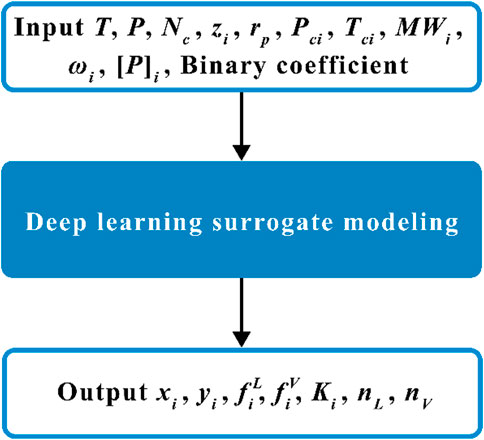
FIGURE 7. Flow char of the surrogate modeling for two-phase flash calculations.

FIGURE 8

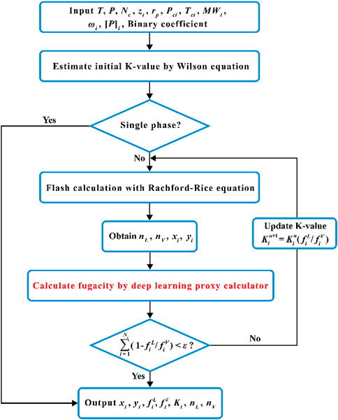
FIGURE 8. Flow char of the DL-FUG modeling for two-phase flash calculations.

FIGURE 9

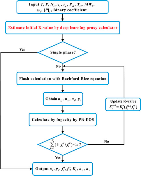
FIGURE 9. Flow char of the DL-KV modeling for two-phase flash calculations.

4.1 Case 1: C₁/C₆/C₁₀

The first case is to validate a three-component fluid mixture that includes C₁, C₆ and C₁₀. Physical parameters of the components are listed in Table 1, and the binary interaction parameters are zero. To generate the big data for the DL-KF modeling based on deep learning methods, the range of the input parameters is present in Table 2. For each component in the fluid mixture, the pressure is range from 0 to 200 bar, and the feed composition space is range from 0 to 1. The pressure intervals in case 1 are set to be 0.5 bar, and the feed composition intervals 0.1. Finally, 1960 data are generated, and the data sets are divided into 80% training data, 10% verification data and 10% test data.

TABLE 1

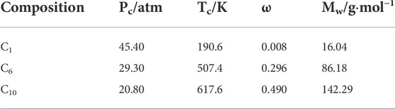
TABLE 1. Physical parameters of components for case 1.

TABLE 2

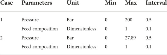
TABLE 2. The range of the input parameters of the training samples.

To validate the proposed DL-KF modeling, original EOS modeling, surrogate modeling, DL-FUG modeling and DL-KV modeling put forward in literatures (Wang et al., 2019b; Yu et al., 2019; Wang et al., 2020) are compared. It is worth noting that the training big data of four deep learning models are all generated by the original EOS modeling, and the calculation results of the original EOS modeling are assumed to be accurate. The results calculated by deep learning models are compared with original EOS modeling to obtain the accuracy and efficiency. The comparison of calculation results for different models are summarized in Table 3. The accuracy calculated by the Mean Percentage Error (MPE):

$\begin{array}{c}MPE=\frac{1}{n}\sum \left|\frac{\mathit{o}-\widehat{\mathit{o}}}{\widehat{\mathit{o}}}\right|\times 100\%\end{array}(17)$

where $n$ is the total number of the predicting data. $\mathit{o}$ is the calculated results from deep learning models. $\widehat{\mathit{o}}$ is the accurate results from the original EOS modeling.

TABLE 3

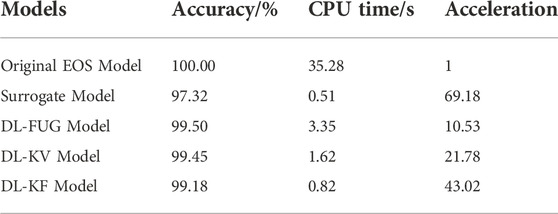
TABLE 3. Comparison of calculation results for different models (196 samples prediction).

As illustrated in Table 3, the surrogate model performs the worst with the accuracy of 97.32%. The DL-KF modeling performs relatively poorly compared with other two deep learning models. This maybe the DL-KF modeling increases the fitting process of the K-values used deep learning methods compared with DL-FUG modeling, and DL-KF modeling increases the fitting process of the fugacity coefficients compared with DL-KV modeling. However, in terms of the overall calculation accuracy, the three deep learning models including DL-FUG modeling, DL-KV modeling and DL-KF modeling have relatively high calculation accuracy.

The efficiency of these models is also investigated. The CPU time of five models is 35.28s, 0.51s, 3.35s, 1.62s and 0.82s respectively. The acceleration times of four deep learning models is 69.18, 10.53, 21.78 and 43.02 compared with the original EOS modeling. The original EOS modeling cost the most and the surrogate modeling takes the least time. This is because the deep learning methods improve computational efficiency. Among the four proposed deep learning algorithms, the surrogate modeling is the fastest due to it is just a fitting of input data and output data, without considering any physical calculation process. In addition, DL-KF modeling performs relatively better compared with other two deep learning models. This is because DL-KF modeling obtained more accurate K-values using deep learning methods which decreases the iteration numbers compared with DL-FUG modeling, and DL-KF modeling reduces the nonlinear calculation process of the fugacity coefficients determined compared with DL-KV modeling. From what has been discussed above, The DL-KF modeling guarantees the calculation accuracy, meanwhile it has high calculation efficiency. Therefore, the DL-KF modeling is better than other four models.

To verify the conservation of component mass during phase equilibrium calculation by the DK-KF modeling, five samples are randomly selected in case 1. As shown in Figure 10, the DL-KF modeling can guarantee the conservation of component mass in liquid and vapor phase, which is crucial for phase equilibrium calculations and reservoir simulation. However, the mass conservation cannot be observed during the phase equilibrium calculations for the surrogate model. In some cases, such as the compositional mole fraction in vapor phase in sample 4, the mass conservation deviation is even greater than 10%.

FIGURE 10

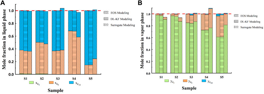
FIGURE 10. Stacked bar chart for compositional mole fraction in liquid phase (A) and vapor phase (B).

4.2 Case 2: C₁/C_2-3/C_4-6/C_7-15/C_16-27/C₂₈₊

A typical 6-component fluid mixture is also investigated. The Physical parameters of the 6-component are listed in Table 4, and the binary interaction parameters are zero. To generate the big data for the DL-KF modeling based on deep learning methods, the range of the input parameters is present in Table 2. Similar to Section 4.1, 65,990 data are generated, and the data sets are also divided into 80% training data, 10% verification data and 10% test data. The structure of neural networks here is the same with that in case 1.

TABLE 4

TABLE 4. Physical parameters of components for case 2.

The comparison of calculation results for different models are shown in Table 5. The accuracy calculated by the MPE. As shown in Table 5, the accuracy of original EOS modeling, surrogate modeling, DL-FUG modeling, DL-KV modeling and DL-KF modeling is 100%, 97.23%, 99.84%, 99.58% and 99.29% respectively. The efficiency is 1250.34s, 6.38s, 29.87s, 26.55s and 7.80s respectively. The acceleration times of four deep learning models is 195.98, 41.86, 47.08 and 160.30 compared with the original EOS modeling. The reasons for these are similar to the analysis for the above case 1 and will not be repeated here. However, it is noted that the efficiency of the deep learning models is improved faster with the increase of fluid components. The more components, the more complex of the traditional flash calculations, and the deep learning models perform better. Furthermore, the DL-KF modeling can also guarantee the conservation of component mass during phase equilibrium calculations. Similar to case 1, it is not stated here for space reasons.

TABLE 5

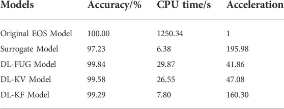
TABLE 5. Comparison of calculation results for different models (6599 samples prediction).

5 Model applications in the oil samples from actual reservoirs

5.1 Model application in an oil sample of C₃H₈-CO₂-heavy oil systems from Huabei oilfield

The DL-KF modeling is applied to calculate the composition concentrations of an oil sample with the C₃H₈-CO₂-heavy oil systems from Huabei oilfield at 1.02MPa and 323.15 K. The physical property parameters and the binary interaction parameters of the oil sample are listed in Tables 6, 7. To generate the big data for the DL-KF modeling, for each component in the fluid mixture, the pressure is range from 0 to 5 MPa, and the feed composition space is range from 0 to 1. The pressure intervals are set to be 0.1 MPa, and the feed composition intervals 0.1. Then the generated model is used to calculate the composition concentrations of Huabei oilfield, and the results are compared with the Peng-Robinson equation of state modeling (PR EOS) proposed in literature (Li et al., 2017). What needs illustration is that the PR EOS modeling is verified with PVT experiments in literature (Li et al., 2017), and it can predict the phase behavior of C₃H₈-CO₂-heavy oil systems with a general good accuracy. As shown in Table 8, the deviation between the DL-KF modeling and the PR EOS modeling is within 5%.

TABLE 6

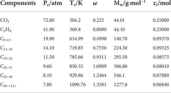
TABLE 6. The physical property parameters of an oil sample of C₃H₈-CO₂-heavy oil systems from Huabei oilfield.

TABLE 7

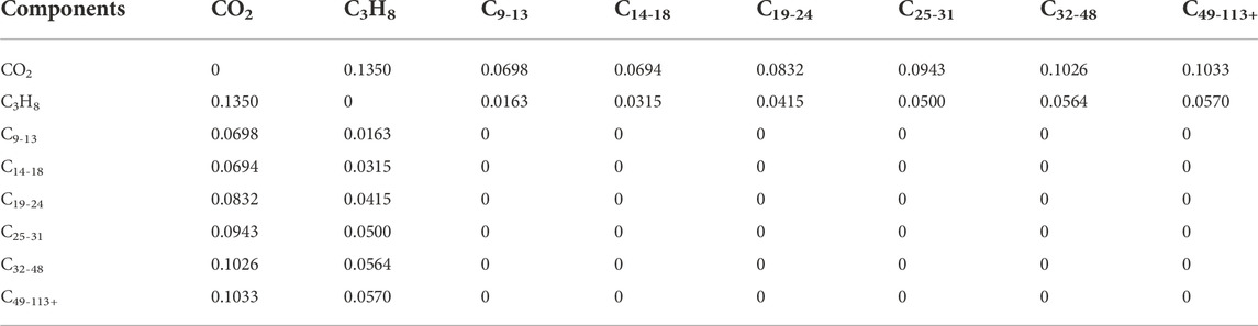
TABLE 7. Binary interaction parameters for fluid components.

TABLE 8

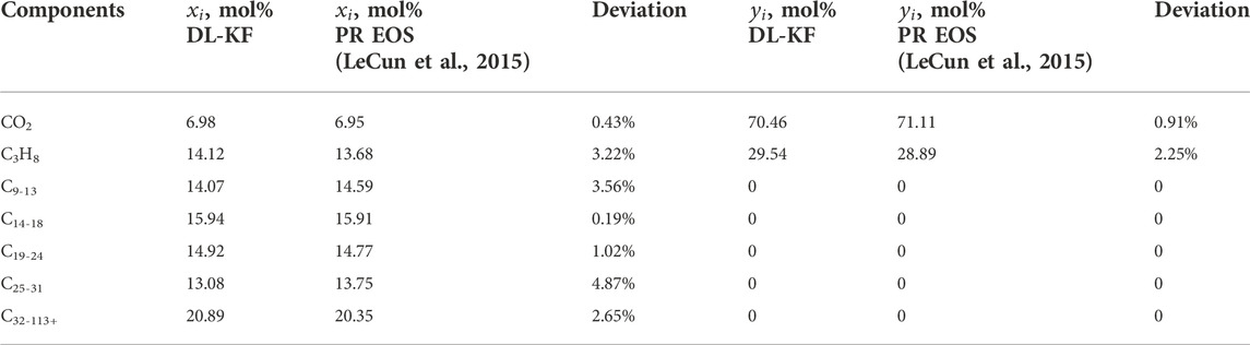
TABLE 8. The comparison results of components concentrations between the DL-KF modeling and PR EOS modeling.

5.2 Model application in CO₂/N₂/hydrocarbons systems of the oil sample in Tahe oilfield

The DL-KF modeling is verified by the PVT experiment of the oil sample in Tahe oilfield. The physical property parameters of CO₂/N₂/hydrocarbons systems and the binary interaction parameters for fluid components are shown in Tables 9, 10, respectively. The temperature of the reservoir fluid of the oil sample in Tahe oilfield is 126.07°C.

TABLE 9

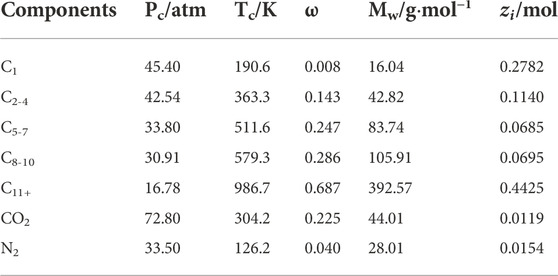
TABLE 9. The physical property parameters of CO₂/N₂/hydrocarbons systems of the oil sample in Tahe oilfield.

TABLE 10

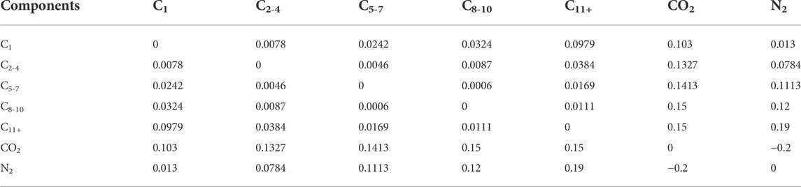
TABLE 10. Binary interaction parameters for fluid components.

The DL-KF modeling is applied in the oil sample from Tahe oilfield. To validate the accuracy of the model, it is used to calculate the physical properties of the crude oil injected with 70% (mole fraction ratio) nitrogen and compared with the experimental results. The viscosity and density of liquid phase and the solution gas-oil ratio of the oil-nitrogen system changes with the system pressure, as shown in Figure 11. The details of calculations of viscosity, density and solution gas-oil ratio can be referred in literature (Zheng et al., 2021). As shown in Figure 11, the deviations between the experimental value and the calculated value are all within 5%.

FIGURE 11

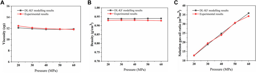
FIGURE 11. Calculation results of the viscosity of liquid phase (A), the density of liquid phase (B) and the solution gas-oil ratio (C) compared between the DL-KF modeling and experiments.

5.3 Model application in the oil sample from Bakken reservoir with CO₂ injection

The DL-KF modeling is applied in the Bakken reservoir with CO₂ injection. Once the composition concentrations are obtained by the DL-KF modeling, the fluid physical properties can be further calculated including phase density, oil volume factor, phase viscosity and solution gas-oil ratio and so on. The fluid physical properties calculations can be referred to reference (Zheng et al., 2021). The composition and physical property parameters of CO₂/hydrocarbons system are taken from Zheng (Zheng et al., 2021). The temperature of the reservoir fluid of the oil sample from Bakken reservoir is 115.56°C.

The fluid phase behavior of Bakken reservoir under 50% (mole fraction ratio) CO₂ injection with corresponding to gas saturation is 0.127 is calculated. The phase mole fraction and composition concentrations are calculated by the DL-KF modeling. In order to validate the accuracy of the model, the results of liquid and vapor mole fraction, mole fraction of components in liquid and vapor phase present in Figure 12 are compared between the DL-KF modeling and original EOS modeling. As can be seen that the results of DL-KF modeling agree well with that of the original EOS modeling.

FIGURE 12

FIGURE 12. Calculation results of the mole fraction compared between the DL-KF modeling and original EOS modeling. (A) The liquid and vapor phase mole fraction. (B) The mole fraction of components in liquid phase. (C) The mole fraction of components in vapor phase.

Figure 13A shows the comparison results of iteration numbers needed to reach the solution between the DL-KF modeling and original EOS modeling. Figure 13B presents the convergence behavior comparison between the DL-KF modeling and original EOS modeling. As can be seen in Figure 13A, the DL-KF modeling’s iteration numbers are reduced by 50.60% with respect to that of the original EOS modeling. The number of iterations decreases more as the pressure increases. As illustrated in Figure 13B, DL-KF modeling converges faster in the convergence behavior. It can be seen from Figure 13, the DL-KF modeling provide a better tool for accelerating phase equilibrium calculation in reservoirs.

FIGURE 13

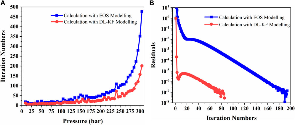
FIGURE 13. Comparison of iteration numbers needed to reach the solution (A) and the convergence behavior (B) between the DL-KF modeling and original EOS modeling.

The oil density of Bakken reservoir under 30%, 50%, 100% (mole fraction ratio) CO₂ injection and no CO₂ injection versus pressure is calculated. As can be seen in Figure 14A, the oil density increases slightly with the increase of gas injection. When the CO₂ injection ratio is 100%, the oil formation volume factor increased by 3.8% compared with that without CO₂ injection at pressure 300 bar. The oil volume factor of Bakken versus pressure is calculated. As shown in Figure 14B, It is obvious that the formation volume factor increases with the increase of gas injection. When the CO₂ injection ratio is 100%, the oil formation volume factor increased by 46.8% compared with that without CO₂ injection at pressure 300 bar. The oil viscosity of Bakken reservoir is also calculated. As shown in Figure 14C, It is obvious that the viscosity decreases with the increase of gas injection. When the CO₂ injection ratio is 100%, the oil viscosity decreased by 62.4% compared with that without CO₂ injection at pressure 300 bar. Hence, CO₂ has obvious viscosity reduction effect. This can be explained by the variation trend of CO₂ solution gas-oil ratio. Gas-oil ratio (GOR) is an important factor in evaluating the degree of gas dissolution. The solution gas-oil ratio of Bakken reservoir versus pressure is shown in Figure 14D. It is obvious that the CO₂ solution gas-oil ratio increases with the increase of gas injection. When the gas injection ratio is 100%, the CO₂ solution gas-oil ratio is about 3 times that of the gas injection ratio is 30%.

FIGURE 14

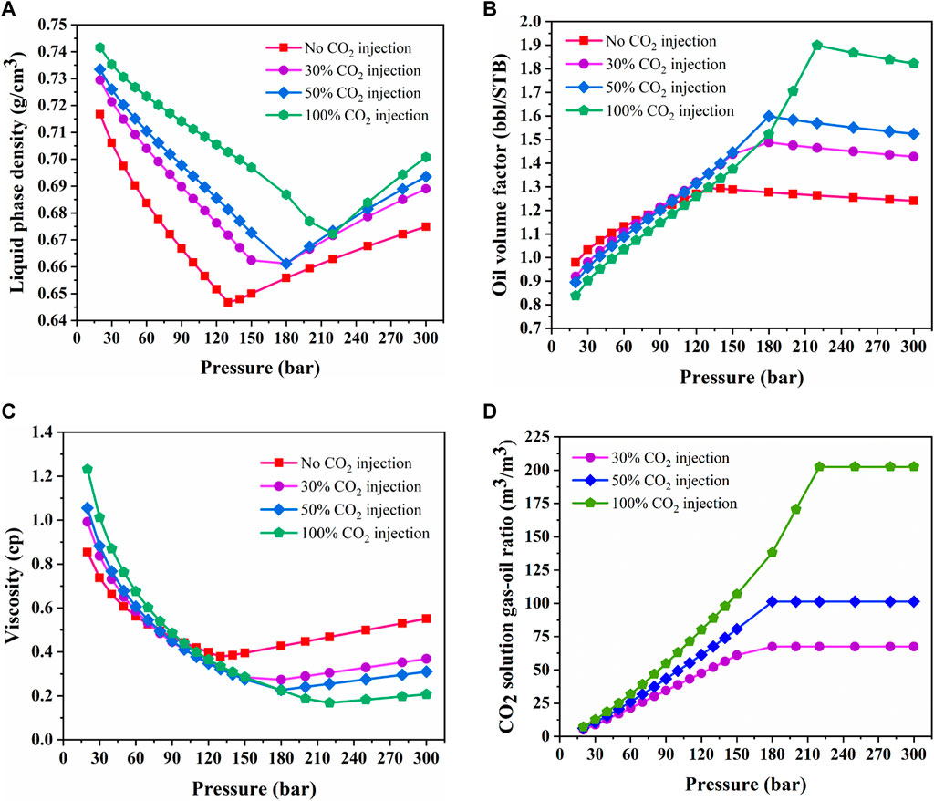
FIGURE 14. Liquid density (A), oil volume factor (B), liquid viscosity (C) and solution gas-oil ratio (D) of Bakken reservoir versus pressure.

6 Conclusion

1) An efficient DL-KF modeling is proposed to accelerate flash calculations. DL-KF modeling constructs based on ANN-STAB model, ANN-KV model and ANN-FUG model. The ANN-STAB model is generated for phase stability test. The ANN-KV model is used for initial K-values determination. The ANN-FUG model is designed for fugacity coefficient calculation. By comparing the performance of deep learning models with different structures, the configuration of each ANN is determined with two hidden layers corresponding to 30 nodes. These three ANN models are embedded into the traditional algorithms to accelerate flash calculations.

2) The proposed DL-KF modeling has been validated and compared with the original EOS modeling, surrogate modeling, DL-FUG modeling and DL-KV modeling on two typical fluid cases. The results indicate that the DL-KF modeling performs best combining computational efficiency and computational precision. In addition, for the fluid with more complex components, the DL-KF modeling based on deep learning methods in accelerating flash calculations in phase equilibrium calculations behaves more obvious. Furthermore, compared with the surrogate modeling, the proposed DL-KF modeling can guarantee the conservation of component mass which is crucial for phase equilibrium calculations and reservoir simulation.

3) The proposed DL-KF modeling is applied in a sample of C₃H₈-CO₂-heavy oil systems from Huabei oilfield, and the deviation of compositions concentrations between the DL-KF modeling and the PR EOS modeling is within 5%. The proposed DL-KF modeling is verified by PVT experiment of an oil sample in Tahe oilfield. The deviations between the experimental value and the calculated value for physical properties are all within 5%. Therefore, the DL-KF modeling is applicable for calculating phase behavior. The model is also applied in an oil sample from Bakken reservoir. The phase mole fraction and composition concentrations are calculated by the DL-KF modeling, and the results of it agree well with that of the original EOS modeling. In addition, the computational performance of the DL-KF modeling is also investigated. The results show that the DL-KF modeling’s iteration numbers are reduced by 50.60% with respect to the original EOS modeling. Meanwhile, the DL-KF modeling converges faster. As can be seen that the DL-KF modeling provides a better tool for accelerating phase equilibrium calculation in reservoirs.

4) The DL-KF modeling is used to investigate the physical properties of Bakken reservoir. Physical properties of Bakken reservoir with 30%, 50%, 100% (mole fraction ratio) CO₂ injection and no CO₂ injection versus pressure is calculated. The oil density increases slightly with the increase of gas injection. When the CO₂ injection ratio is 100%, the oil formation volume factor increased by 3.8% compared with that without CO₂ injection at pressure 300 bar. The formation volume factor increases with the increase of gas injection. When the CO₂ injection ratio is 100%, the oil formation volume factor increased by 46.8% compared with that without CO₂ injection at pressure 300 bar The viscosity decreases with the increase of gas injection. When the CO₂ injection ratio is 100%, the oil viscosity decreased by 62.4% compared with that without CO₂ injection at pressure 300 bar. The CO₂ solution gas-oil ratio increases with the increase of gas injection. When the gas injection ratio is 100%, the CO₂ solution gas-oil ratio is about 3 times that of the gas injection ratio is 30%.

5) In the present work, the fully connected neural network is used for accelerating flash calculations. It needs to be retrained given a new fluid sample. In the future, a self-adaptive deep learning algorithm may also be tried which can make the structure of neural networks to be self-adaptive to the change of different fluid components.

Data availability statement

The original contributions presented in the study are included in the article/Supplementary Material, further inquiries can be directed to the corresponding author.

Author contributions

ZZ: Conceptualization, Methodology, Writing-Reviewing and Editing YD: Supervision EY: Data processing.

Funding

This work is financially supported by the National Key Research and Development Program of China (No. 2018YFA0702400).

Conflict of interest

The authors declare that the research was conducted in the absence of any commercial or financial relationships that could be construed as a potential conflict of interest.

Publisher’s note

All claims expressed in this article are solely those of the authors and do not necessarily represent those of their affiliated organizations, or those of the publisher, the editors and the reviewers. Any product that may be evaluated in this article, or claim that may be made by its manufacturer, is not guaranteed or endorsed by the publisher.

References

Belkadi, A., Yan, W., Michelsen, M. L., and Stenby, E. H. (2011). “Comparison of two methods for speeding up flash calculations in compositional simulations,” in SPE Reservoir Simulation Symposium, Society of Petroleum Engineers. doi:10.2118/142132-MS

CrossRef Full Text | Google Scholar

Bishop, C. M. (2006). Pattern recognition and machine learning. Berlin, Germany: Springer.

Google Scholar

Bottou, L. (2010). “Large-scale machine learning with stochastic gradient descent,” in Proc. COMPSTAT’ 2010 (Heidelberg: Physica-Verlag HD), 177–186. doi:10.1007/978-3-7908-2604-3_16

CrossRef Full Text | Google Scholar

Chollet, F. (2015). Keras, GitHub. Available at: https://github.com/fchollet/keras.

Google Scholar

Firoozabadi, A., and Pan, H. (2000). “Fast and robust algorithm for compositional modeling: Part i-stability analysis testing,” in SPE Annual Technical Conference and Exhibition, Society of Petroleum Engineers. doi:10.2118/77299-PA

CrossRef Full Text | Google Scholar

Gaganis, V., Marinakis, D., and Anna, S. (2021). A soft computing method for rapid phase behavior calculations in fluid flow simulations. J. Petroleum Sci. Eng. 2021 (205), 108796. doi:10.1016/j.petrol.2021.108796

CrossRef Full Text | Google Scholar

Gaganis, V., and Varotsis, N. (2014). An integrated approach for rapid phase behavior calculations in compositional modeling. J. Pet. Sci. Eng. 118, 74–87. doi:10.1016/j.petrol.2014.03.011

CrossRef Full Text | Google Scholar

Hendriks, E. M., and Van Bergen, A. R. D. (1992). Application of a reduction method to phase equilibria calculations. Fluid Phase Equilibria 74, 17–34. doi:10.1016/0378-3812(92)85050-I

CrossRef Full Text | Google Scholar

Jin, Z. L., Liu, Y., and Durlofsky, L. J. (2020). Deep-learning-based surrogate model for reservoir simulation with time-varying well controls. J. Pet. Sci. Eng. 2020 (192), 107273. doi:10.1016/j.petrol.2020.107273

CrossRef Full Text | Google Scholar

LeCun, Y., Bengio, Y., and Hinton, G. (2015). Deep learning. Nature 521 (7553), 436–444. doi:10.1038/nature14539

PubMed Abstract | CrossRef Full Text | Google Scholar

Li, X. L., Han, H. S., Yang, D. Y., Liu, X., and Qin, J. (2017). Phase behavior of C₃H₈-CO₂-heavy oil systems in the presence of aqueous phase under reservoir conditions. Fuel 209, 358–370. doi:10.1016/j.fuel.2017.08.010

CrossRef Full Text | Google Scholar

Li, Y., and Johns, R. T. (2006). Rapid flash calculations for compositional simulation. SPE Reserv. Eval. Eng. 9 (05), 521–529. doi:10.2118/95732-PA

CrossRef Full Text | Google Scholar

Liu, Y., Jin, Z., and Li, H. (2018). Comparison of peng-robinson equation of state with capillary pressure model with engineering density-functional theory in describing the phase behavior of confined hydrocarbons. SPE J. 23 (05), 1784–1797. doi:10.2118/187405-pa

CrossRef Full Text | Google Scholar

Liu, Y., Li, H., and Okuno, R. (2018). Phase behavior of N2/n-C4H10 in a partially confined space derived from shale sample. J. Petroleum Sci. Eng. 160, 442–451. doi:10.1016/j.petrol.2017.10.061

CrossRef Full Text | Google Scholar

Michelsen, M. L. (1986). Simplified flash calculations for cubic equations of state. Ind. Eng. Chem. Proc. Des. Dev. 25 (1), 184–188. doi:10.1021/i200032a029

CrossRef Full Text | Google Scholar

Michelsen, M. L. (1982). The isothermal flash problem. Part II. Phase-split calculation. Fluid Phase Equilib. 9 (9), 21–40. doi:10.1016/0378-3812(82)85002-4

CrossRef Full Text | Google Scholar

Michelsen, M. L. (1982). The isothermal flash problem. Part I. Stability. Fluid Phase Equilib. 9 (9), 21–19. doi:10.1016/0378-3812(82)85001-2

CrossRef Full Text | Google Scholar

Mohamed, M., Guiltinan, E., Vesselinov, V., Middleton, R., Hyman, J. D., Kang, Q., et al. (2021). Machine-learning predictions of the shale wells’ performance. J. Nat. Gas Sci. Eng. 2021 (88), 103819. doi:10.1016/j.jngse.2021.103819

CrossRef Full Text | Google Scholar

Nichita, D. V., Broseta, D., and de Hemptinne, J. C. (2006). Multiphase equilibrium calculation using reduced variables. Fluid phase equilibria 246 (1-2), 15–27. doi:10.1016/j.fluid.2006.05.016

CrossRef Full Text | Google Scholar

Nichita, D. V., Broseta, D., and Montel, F. (2007). Calculation of convergence pressure/temperature and stability test limit loci of mixtures with cubic equations of state. Fluid Phase Equilib. 261 (1-2), 176–184. doi:10.1016/j.fluid.2007.07.041

CrossRef Full Text | Google Scholar

Nichita, D. V., and Graciaa, A. (2011). A new reduction method for phase equilibrium calculations. Fluid Phase Equilibria 302 (1-2), 226–233. doi:10.1016/j.fluid.2010.11.007

CrossRef Full Text | Google Scholar

Nichita, D. V., and Minescu, F. (2004). Efficient phase equilibrium calculation in a reduced flash context. Can. J. Chem. Eng. 82 (6), 1225–1238. doi:10.1002/cjce.5450820610

CrossRef Full Text | Google Scholar

Nojabaei, B., Siripatrachai, N., Johns, R. T., and Ertekin, T. (2016). Effect of large gas-oil capillary pressure on production: A compositionally-extended black oil formulation. J. Pet. Sci. Eng. 147, 317–329. doi:10.1016/j.petrol.2016.05.048

CrossRef Full Text | Google Scholar

Pan, H., and Firoozabadi, A. (2001). “Fast and robust algorithm for compositional modeling: Part ii-two-phase flash computations,” in SPE Annual Technical Conference and Exhibition, Society of Petroleum Engineers. doi:10.2118/87335-PA

CrossRef Full Text | Google Scholar

Peng, D-Y., and Robinson, D. B. (1972). A new two-constant equation of state. Ind. Eng. Chem. Fundam. 51, 385–1082.

Google Scholar

Rachford, H. H., and Rice, J. D. (1952). Procedure for use of electronic digital computers in calculating flash vaporization hydrocarbon equilibrium. J. Pet. Technol. 4 (10), 19–23. doi:10.2118/952327-G

CrossRef Full Text | Google Scholar

Sun, A. Y. (2020). Optimal carbon storage reservoir management through deep reinforcement learning. Appl. Energy 278 (278), 115660. doi:10.1016/j.apenergy.2020.115660

CrossRef Full Text | Google Scholar

Vapnik, V. (2000). The nature of statistical learning theory. Second ed.. New York: Springer.

Google Scholar

Vatandoost, A., Mohammad, R. K. M., and Seyyed, A. M. D. (2016). A new approach for predicting equilibrium ratios of hydrocarbon heavy fractions: Focus on the effect of mixture composition. Fluid Phase Equilibria 410 (410), 42–55. doi:10.1016/j.fluid.2015.11.024

CrossRef Full Text | Google Scholar

Voskov, D., and Tchelepi, H. A. (2007). “Compositional space parameterization for flow simulation,” in SPE Reservoir Simulation Symposium. Society of Petroleum Engineers. doi:10.2118/106029-MS

CrossRef Full Text | Google Scholar

Wang, K., Jia, L., Yizheng, W., Wu, K., Jing, L., and Chen, Z. (2019). Artificial neural network assisted two-phase flash calculations in isothermal and thermal compositional simulations. Fluid Phase Equilib. 486, 59–79. doi:10.1016/j.fluid.2019.01.002

CrossRef Full Text | Google Scholar

Wang, K., Jia, L., Yizheng, W., Wu, K., Jing, L., and Chen, Z. (2020). Practical application of machine learning on fast phase equilibrium calculations in compositional reservoir simulations. J. Comput. Phys. 401, 109013. doi:10.1016/j.jcp.2019.109013

CrossRef Full Text | Google Scholar

Wang, P., and Erling, H. S. (1994). Non-iterative flash calculation algorithm in compositional reservoir simulation. Fluid Phase Equilib. 95 (95), 93–108. doi:10.1016/0378-3812(94)80063-4

CrossRef Full Text | Google Scholar

Wang, S., Qin, C., Feng, Q., Javadpour, F., and Rui, Z. (2021). A framework for predicting the production performance of unconventional resources using deep learning. Appl. Energy 2021 (295), 117016. doi:10.1016/j.apenergy.2021.117016

CrossRef Full Text | Google Scholar

Wang, S., Sobecki, N., Ding, D., Zhu, L., and Wu, Y. S. (2019). Accelerating and stabilizing the vapor-liquid equilibrium (VLE) calculation in compositional simulation of unconventional reservoirs using deep learning based flash calculation. Fuel 253, 209–219. doi:10.1016/j.fuel.2019.05.023

CrossRef Full Text | Google Scholar

Wilson, G. (1968). “A modified Redlich-Kwong EOS, application to general physical data calculations,” in Paper 15C, presented at the Annual AIChE National Meeting, Cleveland, May 4–7, 1968.

Google Scholar

Wilson, G. M. (1964). Vapor-liquid equilibrium. XI. A new expression for the excess free energy of mixing. J. Am. Chem. Soc. 86, 127–130. doi:10.1021/ja01056a002

CrossRef Full Text | Google Scholar

Wu, Y., Kowitz, C., Sun, S., and Salama, A. (2015). Speeding up the flash calculations in two-phase compositional flow simulations – the application of sparse grids. J. Comput. Phys. 285, 88–99. doi:10.1016/j.jcp.2015.01.012

CrossRef Full Text | Google Scholar

Xiao, C., Leeuwenburgh, O., Lin, H., and Arnold, H. (2021). Conditioning of deep-learning surrogate models to image data with application to reservoir characterization. Knowl. Based. Syst. 2021 (220), 106956. doi:10.1016/j.knosys.2021.106956

CrossRef Full Text | Google Scholar

Xiong, Y. (2015). Development of a compositional model fully coupled with geomechanics and its application to tight oil reservoir simulation. Golden, CO, USA: Colorado School of Mines. Arthur Lakes Library.

Google Scholar

Yang, L., Ge, H., Shi, X., Cheng, Y., Zhang, K., Chen, H., et al. (2016). The effect of microstructure and rock mineralogy on water imbibition characteristics in tight reservoirs. J. Nat. Gas. Sci. Eng. 34, 1461–1471. doi:10.1016/j.jngse.2016.01.002

CrossRef Full Text | Google Scholar

Yu, L., Zhang, T., Sun, S., and Gao, X. (2019). Accelerating flash calculation through deep learning methods. J. Comput. Phys. 394, 153–165. doi:10.1016/j.jcp.2019.05.028

CrossRef Full Text | Google Scholar

Zhang, T., Li, Y., Li, Y. T., Sun, S., and Gao, X. (2020). A self-adaptive deep learning algorithm for accelerating multi-component flash calculation. Comput. Methods Appl. Mech. Eng. 369, 113207. doi:10.1016/j.cma.2020.113207

CrossRef Full Text | Google Scholar

Zhang, Y., Yu, W., Sepehrnoori, K., and Di, Y. (2017). Investigation of nanopore confinement on fluid flow in tight reservoirs. J. Pet. Sci. Eng. 150, 265–271. doi:10.1016/j.petrol.2016.11.005

CrossRef Full Text | Google Scholar

Zheng, Z. X., Di, Y., and Wu, Y. S. (2021). Nanopore confinement effect on the phase behavior of CO₂/hydrocarbons in tight oil reservoirs considering capillary pressure, fluid-wall interaction, and molecule adsorption. Geofluids 2021, 1–18. doi:10.1155/2021/2435930

CrossRef Full Text | Google Scholar

Zhu, G., and Li, A. (2020). Interfacial dynamics with soluble surfactants: A phase-field two-phase flow model with variable densities. Adv. Geo-Energ. Res. 4 (1), 86–98. doi:10.26804/ager.2020.01.08

CrossRef Full Text | Google Scholar

Appendix

The PR-EOS is adopted to calculate the fugacity coefficients as follows:

$\begin{array}{c}P=\frac{RT}{V_m-b}-\frac{a}{V_m\left(V_m+b\right)+b\left(V_m-b\right)}\end{array}$(A.1)

where $R$ is gas constant $V_m$ is molar volume. $a$ represents “attraction” parameter. $\mathrm{b}$ is van der Waals co-volume, which represent “repulsion” parameter.

The relationship between compressibility factor Z and pressure P is presented as follows:

$\begin{array}{c}Z=\frac{P{V}_m}{RT}\end{array}$(A.2)

where $Z$ is the compressibility factor.

Hence, Rearranging Eq. A.1 into the compressibility factor form rewrites,

$\begin{array}{c}{Z}^3-\left(1-B\right)Z^2+\left(A-3B^2-2B\right)Z-\left(AB-B^2-B^3\right)=0\end{array}$(A.3)

where,

$\begin{array}{c}A=\frac{{\left(a\alpha \right)}_{m}P}{{\left(RT\right)}^2}\end{array}$(A.4)

$\begin{array}{c}B=\frac{b_{m}P}{RT}\end{array}$(A.5)

For the liquid phase,

$\begin{array}{c}{\left(a\alpha \right)}_m={\displaystyle \sum }_i{\displaystyle \sum }_j\left[x_i{x}_j\sqrt{a_i{a}_j{\alpha }_i{\alpha }_j}\left(1-k_{ij}\right)\right]\end{array}$(A.6)

$\begin{array}{c}{b}_m={\displaystyle \sum }_i\left[x_i{b}_i\right]\end{array}$(A.7)

For the gas phase,

$\begin{array}{c}{\left(a\alpha \right)}_m={\displaystyle \sum }_i{\displaystyle \sum }_j\left[y_i{y}_j\sqrt{a_i{a}_j{\alpha }_i{\alpha }_j}\left(1-k_{ij}\right)\right]\end{array}$(A.8)

$\begin{array}{c}{b}_m={\displaystyle \sum }_i\left[y_i{b}_i\right]\end{array}$(A.9)

The terms $a_i$, $b_i$ and ${\alpha }_i$ are defined as follows as

$\begin{array}{c}{a}_i=0.45724\frac{R^2{T}_{ci}^2}{P_{ci}}\end{array}$(A.10)

$\begin{array}{c}{b}_i=0.07780\frac{R{T}_{ci}}{P_{ci}}\end{array}$(A.11)

$\begin{array}{c}{\alpha }_i={\left[1+m\left(1-\sqrt{\frac{T_{ci}}{T}}\right)\right]}^2\end{array}$(A.12)

where $m=0.3796+1.54226\omega -0.2699{\omega }^2$.

Eq. A.3 can be separately rewritten for liquid phase with the following Eq. A.13.

$\begin{array}{c}{Z}_L^3-\left(1-B_L\right)Z_L^2+\left(A_L-3B_L^2-2B_L\right)Z_L-\left(A_L{B}_L-B_L^2-B_L^3\right)=0\end{array}$(A.13)

where $Z_L$ is the compressibility factor of liquid phase.

Similarly, for vapor phase as follows:

$\begin{array}{c}{Z}_V^3-\left(1-B_V\right)Z_V^2+\left(A_V-3B_V^2-2B_V\right)Z_V-\left(A_V{B}_V-B_V^2-B_V^3\right)=0\end{array}$(A.14)

where $Z_V$ is the compressibility factor of vapor phase.

The fugacity coefficients for liquid and vapor phase are defined by the following expression:

$\begin{array}{c}\ln {\phi }_{\mathrm{i}}^{\mathrm{L}}=-\ln \left[Z_L-B_L\right]+\frac{b_{iL}}{b_L}\left(Z_L-1\right)+\frac{A_L}{2\sqrt{2}{B}_L}\left[\frac{2{\displaystyle \sum }_{i=1}^{N_c}{x}_{jL}\left(1-k_{ij}\right)\sqrt{a_{iL}{a}_{jL}}}{a_L}-\frac{b_{iL}}{b_L}\right]\ln \left[\frac{Z_L+B_L\left(1+\sqrt{2}\right)}{Z_L+B_L\left(1-\sqrt{2}\right)}\right]\end{array}$(A.15)

$\begin{array}{c}\ln {\phi }_{\mathrm{i}}^{\mathrm{V}}=-\ln \left[Z_V-B_V\right]+\frac{b_{iV}}{b_V}\left(Z_V-1\right)+\frac{A_V}{2\sqrt{2}{B}_V}\left[\frac{2{\displaystyle \sum }_{i=1}^{N_c}{x}_{jV}\left(1-k_{ij}\right)\sqrt{a_{iV}{a}_{jV}}}{a_V}-\frac{b_{iV}}{b_V}\right]\ln \left[\frac{Z_V+B_V\left(1+\sqrt{2}\right)}{Z_V+B_V\left(1-\sqrt{2}\right)}\right]\end{array}$(A.16)